Reliability Analysis of Intersection Sight Distance at Roundabouts


1
Department of Civil Engineering; Ryerson University, 350 Victoria Street, Toronto, ON M5B 2K3, Canada
2
School of Transportation, Southeast University, 2 Dongnandaxue Rd, Nanjing 211189, China
3
College of Civil Engineering, Fuzhou University, Fuzhou 350108, China
4
Civil Engineering Department, Sardar Vallabhbhai National Institute of Technology, Surat 395007, India
*
Author to whom correspondence should be addressed.
Infrastructures 2020, 5(8), 67; https://0-doi-org.brum.beds.ac.uk/10.3390/infrastructures5080067
Submission received: 18 July 2020
/
Revised: 3 August 2020
/
Accepted: 4 August 2020
/
Published: 6 August 2020
Abstract
:This paper presents a reliability-based method for the design of intersection sight distance (ISD) at traffic roundabouts using the linear and nonlinear deceleration profiles of the entry vehicles. The reliability method is based on the first-order second moment method which is simple and relatively accurate compared with advanced methods. The nonlinear deceleration profile includes a shape parameter that produces the linear profile as a special case. Deterministic and reliability-based formulas for the required ISD for an approaching vehicle are developed for the entry vehicle on the left and the vehicle on the circulating roadway. Then, the design values of the ISD legs, applicable to any type of roundabout, are presented for different probabilities of non-compliance (Pnc) and different coefficients of variations. For the special case of single-lane symmetrical roundabouts, which have a well-defined geometry, the lateral clearance needs are established. The sensitivity analysis shows that ISD is very sensitive to both the mean and variance of the critical headway. The results show that the deterministic method results in ISD values that correspond to a very small Pnc, indicating that the method is very conservative. The proposed method, which provides flexibility in selecting ISD for any given Pnc, should be of interest to highway designers and practitioners to promote roundabout safety.
1. Introduction
Intersection sight distance (ISD) plays a crucial role in the design of roundabouts. Adequate ISD is required for a driver at each entry of the roundabout to identify safe gaps from conflicting traffic streams. More specifically, ISD should be checked at two locations of the approach vehicle at each entry: (1) a certain distance before the crosswalk and (2) a stationary vehicle at the yield line. Drivers at these locations should clearly see the two conflicting vehicles: circulating and entering from the immediate left. The current methods for calculating ISD are deterministic. Such methods are presented in the roundabout information and design guides by Rodegerdts et al. [1]; the Transportation Association of Canada [2]; the American Association of State Highway and Transportation Officials (AASHTO) [3]; the Federal Highway Administration (FHWA) [4]; the Government of Queensland (GQ) [5]; and the Department for Regional Development, Northern Ireland (DRDNI) [6]. However, the ISD design parameters, such as design speeds, deceleration rate, and critical headway for the conflicting vehicles are random variables in nature instead of fixed values, and they may be correlated with one another.
It has been recognized in the highway engineering field that the reliability-based approach to geometric design can accommodate the uncertainties in the design variables and thus can help improve the overall safety of highways. In the reliability-based (probabilistic) approaches, a safety margin is defined as the difference between the supplied and demanded values of the design element. A negative value of the safety margin would indicate a risk of failure or non-compliance; see Melchers and Beck [7].
Given the flexibility of reliability-based methods, they have been widely used to improve sight distance (SD) design. Table 1 presents a summary of previous reliability-based applications on sight distance and related highway geometric design elements. Examples include general geometric design elements by Navin [8], intergreen intervals at traffic signals by Easa [9], ISD for railway crossings by Easa [10], uncontrolled intersections by Easa [11], freeway entrance speed-change lanes by Fatema and Hassan [12] and Hassan et al. [13], highway cross sections by Ibrahim et al. [14], highway geometric design by Ismail and Sayed [15], truck escape ramps by Greto and Easa [16], and pedestrian green intervals by Easa and Cheng [17]. Most methods have used the first-order second-moment method (FOSM) of reliability analysis, including stop-controlled intersections by Easa and Hussain [18] and left turn at signalized intersections by Hussain and Easa [19]. Other methods have used the advanced version of FOSM (AFOSM) [10,16]. The more advanced first-order method (FORM) has been used by several authors, including Osama et al. [20], Richl and Sayed [21], De Santos-Berbe et al. [22], and Llorca et al. [23]. In addition, some researchers have used Monte Carlo (MC) simulation, such as El-Khoury and Hobeika [24] who studied passing sight distance (PSD) on two-lane highways; Sarhan and Hassan [25], who studied sight distance on three-dimensional highway alignments; Wood and Donnell [26], who studied sight distance on horizontal curves; and Andrade-Catano et al. [27], who studies headlight sight distance on sag vertical curves. MC simulation has also been used in some studies to verify the assumptions of the analytical reliability methods [17].
From Table 1, it is noted that many efforts in the literature have focused on the SD along highways and at intersections. Only a few studies have focused on SD design at roundabouts, such as Faizi and Easa [28]. In this paper, the authors proposed a reliability-based approach for optimizing the deterministic stopping sight distance (SSD) model recommended by AASHTO [3]. The stopping sight distance at three locations was addressed—roundabout approach, circulatory roadway, and roundabout exit—while the ISD was not considered. Therefore, a comprehensive probabilistic approach for the design of ISD at roundabouts is currently lacking. To address this knowledge gap, the objectives of this paper are fourfold: (1) to develop a reliability-based method for the design of ISD at roundabouts, (2) to formulate a nonlinear deceleration profile for the entry vehicles at roundabouts for ISD, (3) to develop reliability-based ISD design values that are applicable to any type of roundabout, and (4) to develop lateral clearance needs for the special case of single-lane symmetrical roundabouts.
2. Deterministic ISD with Nonlinear Deceleration
2.1. Modeling Nonlinear Deceleration Profile
The deceleration profiles are formulated for the entry vehicles which decelerate from the entry speed ve to the circulating speed vc. The analysis concept is based on a comparison of the kinematic equations associated with the deceleration rate. The concept is like that given by Wortman and Fox [29], who developed the deceleration profiles for stopping vehicles (vc = 0). The stopping deceleration profile is a special case of the presented general formulation of deceleration profiles. Let the deceleration distance and deceleration time be denoted by d and t, respectively. Three basic equations are used to calculate the deceleration rate, where each equation is a function of two of the variables (ve, vc, d, and t), as follows:
where a1, a2, and a3 denote the deceleration rate (m/s2) that corresponds to Equations (1)–(3), respectively; ve and vc denote the entry and circulatory speeds (m/s); d denotes the deceleration distance (m); and t denotes the deceleration time (s).
Note that, to simplify the presented formulas, the speeds are in m/s, but the design aids presented later will make appropriate conversion of these speeds to km/h. For linear deceleration, a1 = a2 = a3. For nonlinear deceleration, however, the deceleration rates of Equations (1)–(3) will be different. The different cases of the deceleration profiles are quantified as follows:
where r denotes the deceleration shape parameter. The deceleration rates a1 and a2 are used because for nonlinear deceleration profiles they represent limiting values, where a3 always lies between them. That is, there are two possible inequalities a1 < a3 < a2 and a2 < a3 < a1, which correspond to r < 1 and r > 1, respectively. For linear deceleration profiles, r = 1.
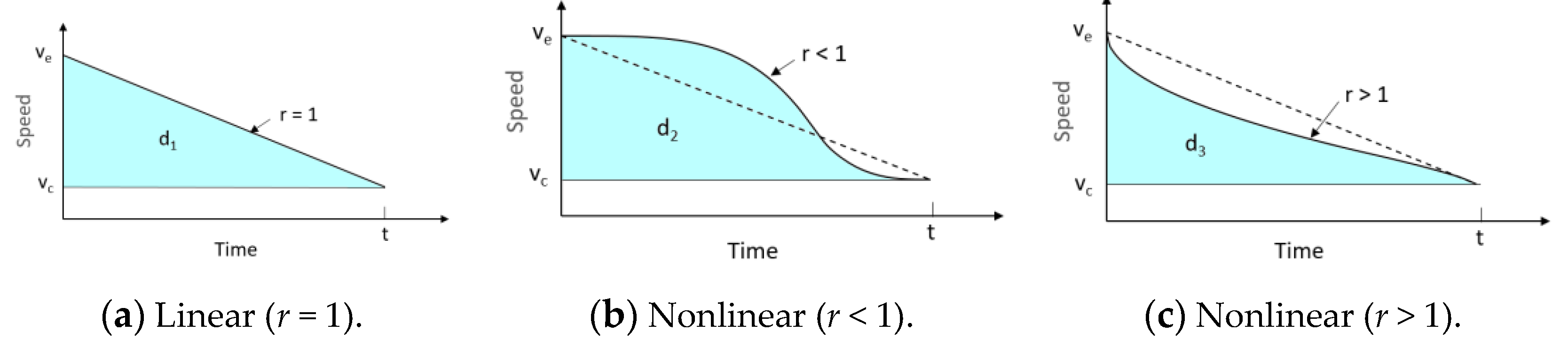
The three possible deceleration profiles are shown in Figure 1. The time axis is the elapsed time from the start of the deceleration. The speed axis identifies the speed of the vehicle. The area under the curve is the distance over which the deceleration occurs. The slope of the curve at any point is the deceleration rate. Figure 1a represents linear deceleration (r = 1), and the area under the curve is d1. Figure 1b,c represent the nonlinear deceleration rate when r < 1 and r > 1, respectively, with the corresponding areas d2 and d3 (d2 > d1 > d3). Note that the deceleration profile of Figure 1b starts with a gentle deceleration rate followed by a more aggressive rate, covering a larger distance (during the same time t) than that of linear decelerate rate. This behavior would be expected at a low entry speed with a large circulatory speed. On the other hand, the deceleration profile of Figure 1c starts with a more aggressive rate followed by a gentler rate, covering a smaller distance (during the same time t) than that of the linear decelerate rate. This behavior is expected at a high entry speed with a low circulatory speed.
The distance travelled for each deceleration profile is needed for calculating the sight distance leg of ISD to the entry vehicle. To derive this distance, substituting a1 and a2 into Equation (4), then:
where, based on Equation (3), t is given by:
As noted, Equation (5) is a quadratic function in d. Solving this equation yields:
For linear deceleration (r = 1), Equation (7) gives:
This is the well-known formula for the distance travelled during linear deceleration.
2.2. Formulas for Sight Distance Legs
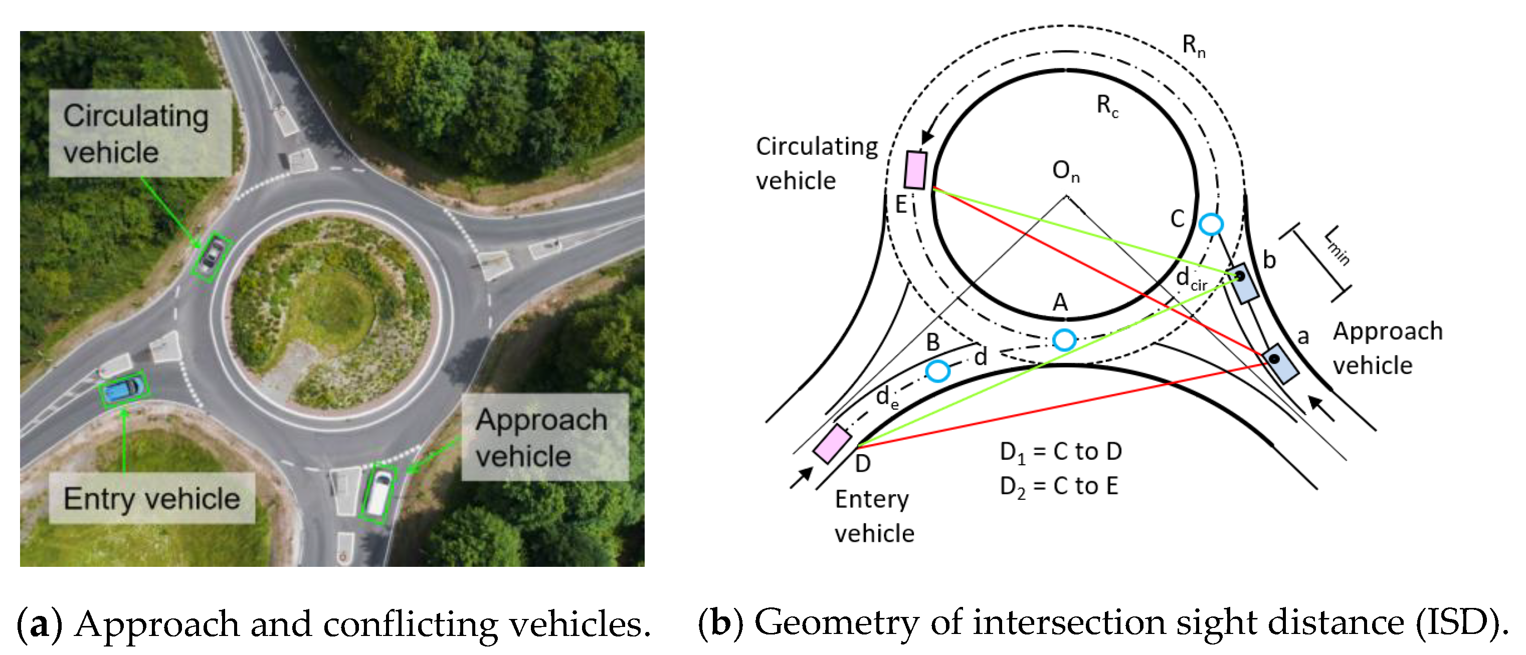
The ISD is checked at each entry of the roundabout, generally at two locations of the approach (Figure 2): at a specified minimum distance from the yield line (typically Lmin = 15 m) and at the yield line. At each entry, the sight distance triangle has two conflicting approaches that must be checked independently: (1) conflicting vehicles within the circulatory roadway (left-turn movements from the opposing entry approach) and (2) conflicting vehicles from the immediate upstream entry (left-turn or through movements).
A sight distance triangle that allows a driver to see and safely react to the conflicting vehicles is established. This triangle has three sides: the approach leg, the conflicting vehicle leg, and a line connecting these two limits (sightline). The approach leg (line from the driver’s eye to the conflict point) is the same for both conflicting streams. For example, for an approach vehicle at Lmin from the yield line, the approach leg is aC. For the conflicting-entry vehicle, the conflicting leg is CD (or D1) and the third leg is the sightline aD. For the conflicting-circulating vehicle, the approach leg is bC, the conflicting leg is CE (or D2), and the third leg is the sightline bE. The conflicting leg of the sight triangle should follow the conflicting-vehicle curved path; see Rodegerdts et al. [1,30,31].
In general, the sight distance leg of the entry vehicle (distance from the conflict point to the entry vehicle), D1, is given by (Figure 2b):
where dcir denotes the distance along the circulatory part of the path; d denotes the distance during deceleration, given by Equation (7); and de denotes the distance along the entry curve. The distance de equals the entry speed ve multiplied by the time te, which corresponds to de.
Note that dcir depends on the minimum radius of the circulatory roadway R (which depends on vc), and the central angle suspended by this portion of the path (assumed to be 30°, based on the visual inspection of numerous roundabouts). The minimum radius was calculated based on the lateral friction coefficients for urban low speeds and e = 0.02 [3]. For the reliability analysis, based on AASHTO data, the relation between R and vc was established using regression analysis as:
where R = the radius of the circulatory roadway (m) and vc = the design speed of the circulatory roadway (m/s). Then, the portion of the entry vehicle path on the circulatory roadway, which equals (where the angle is in radians), is given by:
The time spent by the entry vehicle on the circulatory roadway equals dcir/vc. Thus,
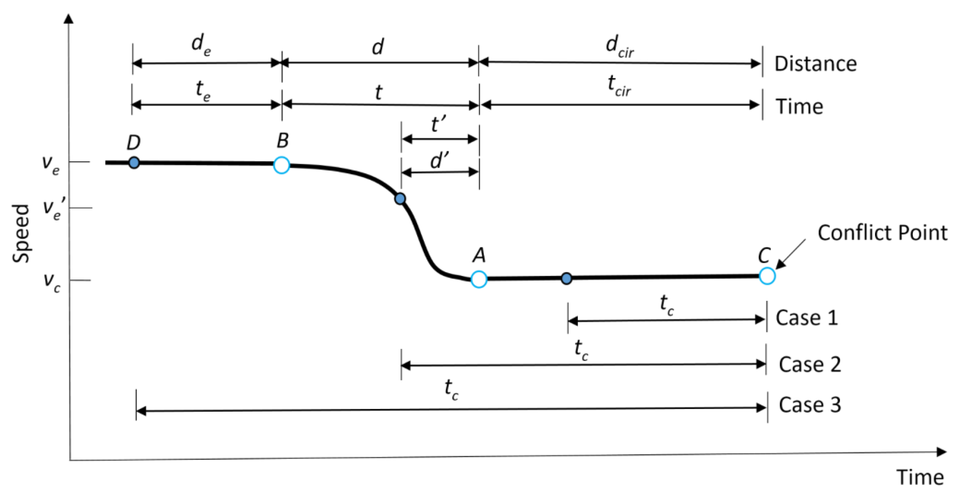
There are three possible cases for calculating D1, as shown in Figure 3. The three cases are formulated as follows:
Case 1: The end of the sight distance leg lies on the circulatory part of the entry path. In this case, the critical headway is less than or equal to the time spent on the circulatory portion of the entry vehicle path (tc ≤ tcir). In this case, D1 is given by:
Case 2: The end of the sight distance leg lies on the deceleration part of the entry path. In this case, the critical headway greater than the time on the circulatory part but is less than the sum of the times on the circulatory and the deceleration parts (tcir < tc < tcir + t). To calculate D1 in this case, let the time corresponding to the part on the deceleration profile be denoted as t’ and the corresponding speed of the entry vehicle at the end of D1 be . Then,
Based on Equation (14), is given by:
Then, D1 can be derived as:
where the second part of Equation (16) is the part of D1 on the deceleration profile (d’).
Case 3: The end of the sight distance leg lies on the entry part before deceleration. In this case, the critical headway is greater than the sum of the times on the circulatory and deceleration parts (tc ≥ tcir + t). The time on the entry part equals the critical headway time tc minus the time spent on the deceleration and the circulatory parts. Thus, D1 can be derived as:
Note that for r = 1 (linear deceleration), Equation (17) becomes:
This is the deterministic formula of D1 for the linear deceleration rates.
For the circulating vehicle, the length of the conflicting leg is given by:
where D2 denotes the length of the sight distance leg for the conflicting circulating vehicle (m), tc = the critical headway for entering the roundabout (s), and vc = the design speed of the conflicting circulating vehicle (km/h). Note that Equation (20) is equivalent to the sight distance leg for the entry vehicle of Case 2.
The effect of the deceleration shape parameter on the sight distance D1 was calculated for different values of r (0.5, 1, and 1.5) for the deterministic case. Different combinations of entry speed (Ve = 30 km/h to 70 km/h) and circulatory speed (Vc = 20 km/h to 60 km/h) and the 90th percentile value of tc and the 10th percentile value of a were used. The results are presented in Table 2. As noted, for r = 0.5 the difference in D1 between the linear and nonlinear profiles reaches up to 19.3%, and for r = 1.5 the difference reaches up to −8.1%. Obviously, when Ve = Vc, there is no deceleration, and the difference equals zero.
3. Proposed Reliability Method
3.1. FOSM Reliability Method
The FOSM method is simpler and more straightforward than other advanced methods. In this method, a performance function is expanded at the mean values of the random variables. Let the safety margin, SM, be a nonlinear performance function that involves several random variables, xi, i = 1, 2, …, n. Then,
The FOSM method uses a Taylor series expansion about the mean values of the random variables, and expresses the mean and variance of the random variable SM, E[SM], and var[SM], respectively, as follows:
where μxi = the mean of the random variable xi, σxi2 = the variance of the random variable xi, σxi = the standard deviation of the random variable xi, and ρxi, xj = Pearson’s coefficient of the correlation between xi and xj. Furthermore, the coefficient of variation of the random variable xi, CVxi, which is a dimensionless measure of dispersion, is given by:
The reliability index,, defines the number of standard deviations between the expected value of SM and the limit state, SM = 0. That is,
Assuming that SM is normally distributed, Pnc can be estimated as:
where Φ(−β) = the area under the standard normal variate PDF (probability distribution function) from – ∞ to – β, obtained using standard normal variate tables. For example, for β = 1.64, Pnc = 5%. The larger β is, the smaller the Pnc. If SM is linear, the mean and standard deviation will be accurately assessed using the FOSM method. However, if SM is nonlinear, the FOSM analysis may introduce errors. For more details about reliability analysis, the reader is referred to Benjamin and Cornell [32], Smith [33], and Haukaas [34].
3.2. Reliability Analysis of ISD
3.2.1. Distance D1
The safety margin is defined as the difference between the supplied and demanded length of the sight distance leg to the entry vehicle. That is,
where denotes the length of D1 supplied (m) and = the length of D1 demanded (m), which equals D1 from Equations (13), (16), and (17) for Cases 1–3, respectively. In general, the expected value and variance of the SM1, and var[SM1], based on Equations (22) and (23), are given by:
where = the expected value of the demanded sight distance D1, which is obtained by substituting the mean values of the component random variables into the D1 equation of the respective case. Note that Equation (29) includes the correlations between several variables: (ve, tc), (ve, a), (ve, r), and (vc, a). The first three correlations are positive, while the fourth is negative. The first derivatives are given next for the three cases.
Case 1:
Substituting D1 from Equation (13) into Equation (27), the first derivatives of with respect to can be derived as:
where denotes the mean of the indicated random variable.
Case 2:
Substituting t’ and ve’ from Equations (14) and (15) and dcir and tcir from Equations (11) and (12) into Equation (16), then substituting D1 into Equation (27), the first derivatives of with respect to can be derived as:
where .
Case 3:
Substituting t and dcir from Equations (5) and (11) into Equation (17), then substituting D1 into Equation (27), the first derivatives of with respect to can be derived as
where . Based on Equations (25) and (28), then:
Then, D1supply is calculated for various values of Pnc. Note that the conditions for the three cases presented previously involves random variables, and therefore these conditions also involve uncertainty. The probabilistic equivalent of the deterministic conditions for the three cases are presented in Appendix A.
3.2.2. Distance D2
The safety margin, defined as the difference between the supplied and demanded lengths of the sight distance leg to the circulating vehicle, is given by:
where denotes the length of D2 supplied (m) and = the length of D2 demanded (m), which equals D2 from Equation (19). Then,
where the random variables are The expected value and variance of the SM2, and var[SM2], based on Equations (21) and (22), are given by:
where the first derivatives with respect to vc and tc are given by the right sides of Equations (30) and (31), respectively. Based on Equations (25) and (44), then:
Then, D2supply is calculated for various values of Pnc.
3.3. Verification
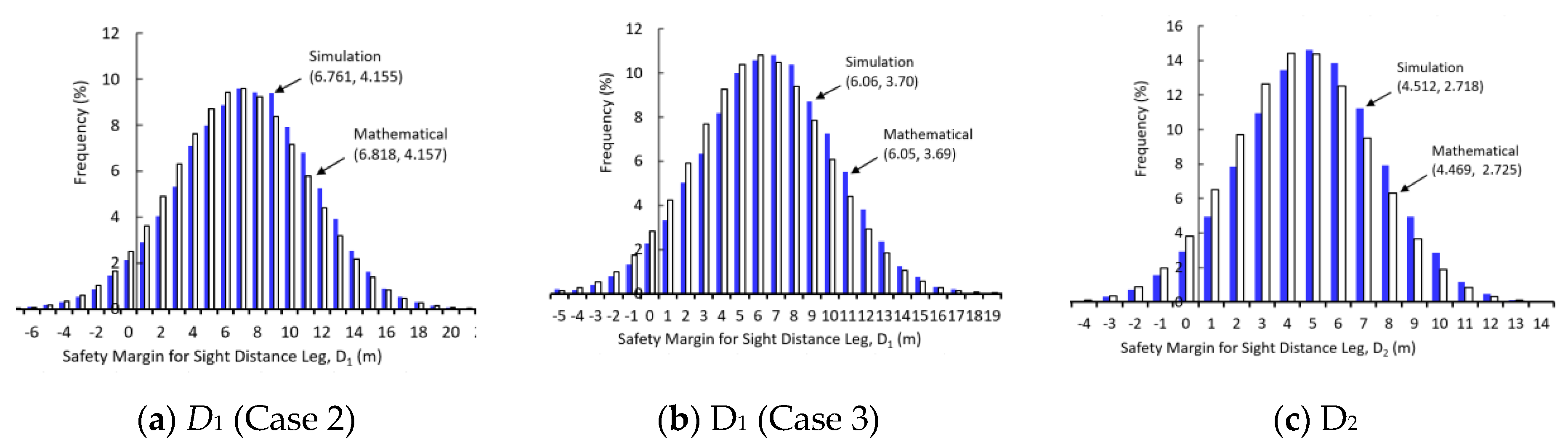
The proposed reliability methods for D1 and D2 were verified using Monte Carlo simulation. The probability distribution of the safety margin of the mathematical method, based on ], var[SM1], and ], var[SM2] was compared with that of the simulation. The mean values of the random variables were as follows. For D1 (Case 1), µve = 12.85 m/s and µvc = 10.28 m/s, and for D1 (Case 2), µve = 12.85 m/s and µvc = 7.71 m/s. For both cases, µtc = 5 s, µa = 1.3 m/s2, and µr = 0.5. The coefficient of variation was 5% for all variables. The mean entry and circulatory speeds correspond to the design speeds of 50 km/h and 40 km/h, respectively, which were assumed to represent the 95% percentile speed, as discussed later in data preparation. For D2, µvc = 7.71 m/s and µtc = 5 s with coefficient of variation (CV) = 5%, where the mean circulatory speed corresponds to a design speed of 30 km/h. All the random variables were assumed to be normally distributed in the simulation. For simplicity, the variables were assumed to be uncorrelated. Note that the FOSM reliability method requires no assumptions about the distributions of the input random variables.
The simulation involved generating 30,000 random values of the component random variables of the respective equations for D1 (ve, vc, tc, a, and r) and D2 (vc, tc). The probability distributions of the component random variables were assumed to be normal, with the means and standard deviations calculated from the data. The generated random values of the component variables were then substituted into the respective equations, resulting in 30,000 values of the dependent random variable. Using these values, their means and standard deviations were calculated along with their histograms. The reliability index was β = 1.64 (Pnc = 5%). For D1 (Case 2), the mean and standard deviation of the safety margin of the mathematical model were ], = 6.818 m and σSM1 = 4.157 m, compared with the simulation values of 6.761 and 4.155 (Figure 4a). The results for Case 3 were also very close (Figure 4b). For D2, the mathematical and simulated values were (4.469, 2.725) and (4.512, 2.718), respectively (Figure 4c). As noted, the means and standard deviations of the simulation and mathematical formulas show excellent agreement. In particular, the close standard deviations of the mathematical and simulation methods verify the rather complex first derivatives of Cases 2 and 3 of D1. In addition, the simulation results show that the probability distributions of the design variables are very close to the normal distribution.
4. Application
4.1. Data Preparation
Data related to the means and standard deviations of the component random variables are required for the application of reliability methods. Most data were determined from the percentile values of the random variables reported in the literature. For normally distributed random variables, the relationship between the mean and extreme value is given by Hussain and Easa [26] as:
where μXi denotes the mean of the random variable xi, Exi denotes the extreme value corresponding to a certain percentile value of the random variable xi, z denotes the number of standard deviations of the normal distribution corresponding to a certain percentile value, and CVXi denotes the coefficient of variation of the random variable. Note that z is positive for variables for which the extreme values are based on a high percentile value and negative when low percentile values should be used. For example, the value of z for a random variable with respect to its 95th percentile value is 1.64 and −1.64 for the 5th percentile.
Table 3 shows the selected values for various random variables that were used for establishing the design aids. The 95th percentile values represented the design speeds of Ve, Vc, and tc. On the other hand, the 10th percentile value represented the design value for a, since smaller values of the deceleration rate result in larger values of D1. For the deceleration shape parameter, there is currently no guidance for the roundabout deceleration profile (without stopping). However, previous research on vehicle stopping [29] showed that the value of r ranged from 0.4 to 1.7, where the approach speed for r = 1 was 77.2 km/h (48 mph). Speeds less than this limiting value corresponded to r < 1, and speeds larger than this value corresponded to r > 1. Since the entry speeds for roundabouts are typically less than 70 km/h, two values were selected for establishing the design aids: r = 0.5 (nonlinear deceleration) and r = 1 (linear deceleration).
4.2. Design Values of ISD
Design values of D1 and D2 were established using the reliability-based method of Equations (41) and (46), respectively, for CV = 5% and 10% and Pnc = 1%, 5%, and 10%. For D1, the values were established for different combinations of Ve and Vc and for linear (r = 0.5) and nonlinear (r = 1.0) deceleration profiles, as shown in Table 4. As noted, larger design values are required for a larger CV and smaller Pnc. The deterministic values are also shown in the table. A comparison of the deterministic and reliability-based values for Ve = 60 km/h of Table 4 are shown graphically in Figure 5. As noted, the deterministic values correspond to a low probability of non-compliance (about Pnc = 1%), indicating that such values are conservative. This finding is consistent with that of Easa [23], where the deterministic values for uncontrolled intersections corresponded to a very small probability of non-compliance. This is not surprising, since the deterministic method uses very high or very low percentile values (depending on the nature of the random variable). Note also that the trends of the design values for the linear and nonlinear deceleration profiles are similar, except that the values for the nonlinear profile (r = 0.5) are greater, as previously discussed.
The design values for D2 are shown in Table 5 for Vc ranging from 20 to 60 km/h. As noted, similarly to D1, the deterministic values also lie close to the reliability-based values for Pnc = 1%. Note that the design values of D1 and D2 do not depend on any specific geometric configuration of the roundabout, and therefore they are applicable to all types of roundabouts. Only D1 depends on the minimum radius of a circulatory roadway.
4.3. Lateral Clearance Needs: Special Case
Although the design values of ISD are applicable to any type of roundabout, the lateral clearance needs would vary from one roundabout to another depending on its specific geometry. Only in the special case of single-lane symmetrical roundabouts can lateral clearance needs be mathematically formulated [35]. Note that the lateral clearance formulation in that paper is general and is applicable to any values of ISD (deterministic or reliability-based). For a single-lane symmetrical roundabout, the relation between the entry radius and the radius of the inscribed circle can be derived as:
where R1 = the entry radius (m), Rc = the circulatory roadway radius (m), wc = the circulatory roadway width, α = the angle between the y-axis and the line connecting the centers of the entry and inscribed circle curves (45°), and w1 = the distance from the curb to the centerline of the road (m). The inscribed circle radius Rn = Rc + wc. Given Rc and w1, R1 is calculated using Equation (48).
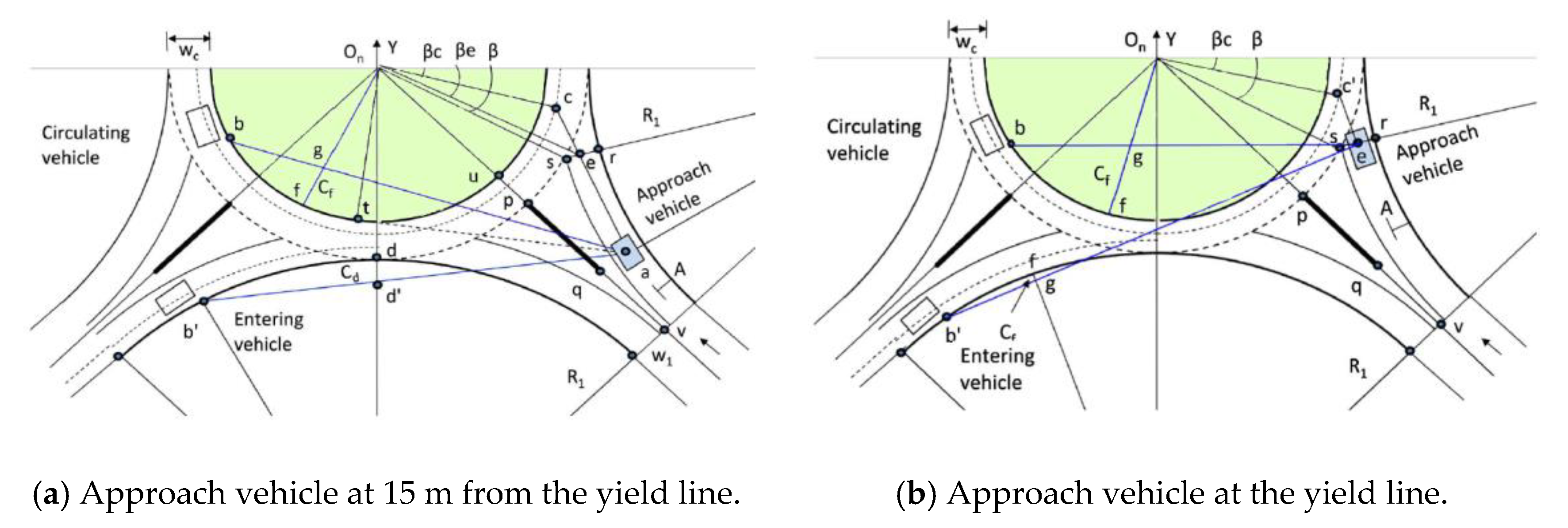
The geometry of the lateral clearance for a single-lane symmetrical roundabout is shown in Figure 6 for an approach vehicle at the yield line and at 15 m from the yield line. Given the design values presented in the previous section for the two cases, the corresponding lateral clearance for each case was determined. As noted in Figure 6a (vehicle at 15 m from the yield line), the lateral clearance for the sight line ab’ to the entry vehicle on the left, Cd, is determined at the tangential point d. For the conflicting circulating vehicle, the maximum lateral clearance for the sight line ab is determined. For the conflicting-entering vehicle, after the formulation of the general lateral clearance Cf, the maximum lateral clearance is determined using optimization as follows:
This is subject to:
where df denotes the distance of Point f on the central island curb (decision variable), measured from the road centerline (Point u), and dL and dU denote the arbitrary lower and upper limits of the decision variable, respectively, that cover the possible range of lateral clearance and can be set up in different ways.
In this study, they were set equal to 0 and the distance on the curb from Point u to Point b, respectively. Note that the lateral clearance for the central island implies a clear zone where the height of the landscaping and other objects around the outer edge of the central island will be restricted. The driver’s eye and object heights should both be 1.08 m. The lateral clearance for a vehicle at the yield line (Figure 6b) is determined similarly. The detailed formulation of lateral clearance can be found in Easa [35]. Based on Equations (49) and (50), the lateral clearance needs to the entry vehicle (based on D1 of Table 4) and to the circulating vehicle (based on D2 of Table 5) are presented in Table 6 and Table 7. For D1, the values of Table 6 correspond to the lateral clearance, Cd, at the tangent point d for the sight line ab’ (Figure 6a). For D2, the values of Table 7 correspond to the maximum lateral clearance on the central island for the sight line eb (Figure 6b).
4.4. Sensitivity Analysis
A sensitivity analysis was conducted to determine how sensitive the required sight distance is to various input variables. For D1, the input data for the base case were Ve = 50 km/h, Vc = 30 km/h, tc = 5 s, a = 1.3 m/s2, and r = 1, where a capital letter V indicates the speed in km/h. The coefficient of the variation of all variables was 5%, and the correlations were = 0.5, = 0.5, = 0.5, = 0.5, and = −0.5. The probability of non-compliance was Pnc = 5%. One variable of the base scenario was changed at a time, while keeping all other variables at their base values. The mean values were increased by 10%, the CV was increased to 10%, and the correlations were changed to 0.8.
The results of the sensitivity analysis are shown in Table 8. As noted, the sight distance D1 is very sensitive to the mean value of tc and somewhat sensitive to that of Ve. The value of D1 is also very sensitive to the coefficient of variation of both Vc and tc and somewhat sensitive to that of Ve. The sight distance is somewhat sensitive to the values of the correlation coefficients. In addition, the results show that D2 is sensitive to the mean values of Vc and tc and to the coefficient of variation of tc. Clearly, the mean value and variability of tc substantially affect the ISD and should be accurately determined. In addition, the variability of the circulatory speed is an important variable. Other variables including the correlations have little or moderate effects on the calculated sight distance.
5. Conclusions
The paper has presented a general reliability-based method for roundabout intersection sight distance that is applicable to linear and nonlinear deceleration profiles. The required sight distances to the entry vehicle on the left and the vehicle on the circulatory roadway were modeled using the first-order second moment method of reliability analysis. Based on this study, the following comments are offered:
The developed design values of the ISD legs are applicable to any type of roundabout (with a circular central island). However, the developed lateral clearance needs are applicable only to the special case of single-lane symmetrical roundabouts that have a well-defined and simple relationship between the entry and circulatory curves. The lateral clearance needs for other complex roundabouts can be established graphically using the developed ISD values. It should also be noted that the proposed reliability-based model is basically relevant for right-hand driving. The model implements an extended formula of the entry vehicle ISD, which explicitly incorporates the deceleration rate. This formula is based on North American practice [1]. However, the concept of the proposed model can be applied to left-hand driving, which normally implements a different formula for the entry vehicle ISD.
Reliability-based design values for the required ISD for different probabilities of non-compliance and different coefficients of variation were established in this paper. These design values are applicable to any geometry of roundabouts, including symmetrical, skewed, or staggered roundabouts. For D1, the only requirement is that the central island should be circular, since the design values are based on a distance around circular central island. The values were based on the minimum radius that corresponds to the design speed of the circulatory roadway. However, the design values can perhaps be used with flatter radii of the central island than the minimum values, since they correspond to smaller lateral clearance needs.
The lateral clearance needs for a vehicle at the yield line or 15 m from the yield line cannot be generally calculated mathematically, since there are many variations in roundabout geometry. Using the design values of ISD presented in this paper can be used to determine the required lateral clearances graphically or using roundabout software. However, for single-lane roundabouts, which have a well-defined geometry, the lateral clearance needs for the entry and circulatory vehicles are presented in this paper. Note that the lateral clearance needs for the circulatory vehicle were established based on an approach vehicle at the yield line, while those for the entry vehicle were established for an approach vehicle at 15 m from the yield line, since these locations provide the maximum values [35].
The variabilities of the design variables affect the ISD needs, where a larger coefficient of variation requires a larger ISD length. The mean and variance of the critical headway was the variable that impacted the ISD needs the most. In addition, the existing deterministic method, where the design speeds and percentile values of the critical headway and deceleration rate are used, is very conservative and corresponds to very small values of the probability of non-compliance. In terms of design and regulatory innovations, the proposed method provides the designer with flexibility in cases where the lateral clearance is restricted in the field. In this case, different ISD (and in turn lateral clearance) values corresponding to different reliability levels are available to designers. In addition, speed control alternatives can be explored to maintain satisfactory ISD requirements for the approach vehicles.
More advanced reliability methods, such as AFOSM can be applied to analyze sight distance at roundabouts, however, the results of the FOSM method were close to those of the AFOSM based on an analysis not reported in this paper. In addition, previous research by Greto and Easa [15] showed a difference of generally less than 5% between the two methods. Given the fact that the non-compliance of ISD needs at roundabouts does not pose a catastrophic event, the application of the simple, straightforward FOSM method is justified.
The FOSM reliability method assumes that the safety margin is normally distributed. This assumption is quite reasonable. According to the Central Limit Theorem, when a variable is a function of several random variables, its probability distribution tends to be normal, regardless of the types of the probability distributions of the component random variables [32]. This assumption was verified in this paper using Monte Carlo simulation. In addition, the simulation has also verified the developed mathematical method of ISD reliability analysis.
In setting up the sightline from the approach vehicle to the entry vehicle on the left, the distance D1 from the conflict point to the entry vehicle should be calculated. The Australian guide assumes that the entry vehicle travels at the entry speed for the entire leg [5]. Rodegerdts et al. [1] implemented a more realistic assumption by considering that the entry vehicle travels to the conflict point at the average of the Ve and Vc. Both assumptions would result in conservative later clearance needs. This assumption was subsequently revised by Easa [35] by assuming that the entry vehicle travels at the average of the entry and circulatory speeds prior to reaching the circulatory path. In this case, the use of the average speed would indirectly account for the deceleration that occurred before reaching the circulatory path. The present paper has further improved the modeling of the entry-vehicle deceleration by explicitly considering the vehicle deceleration profile of the entry vehicle. Note that setting up the sightline based on the proposed method would be conservative for other entry vehicles from the left that stop at the yield line and 15 m from the yield line.
There is currently no guidance regarding the selection of the deceleration shape parameter r for roundabout entry vehicles that decelerate from the entry to the circulatory speeds. For roundabouts, where the design speeds are relatively small, the shape parameter is expected to be less than 1. For this case, the results showed that the nonlinear deceleration rate may require up to 20% greater sight distance for the entry vehicle than that of the linear case. The authors are currently conducting research to establish design values for the deceleration shape parameter. A relation that expresses the deceleration parameter as a function of Ve and Vc is being established using measurements from drone and video-based trajectory data.
Author Contributions
Conceptualization: S.M.E.; Methodology: S.M.E., S.L., Y.M.; Formal analysis: S.M.E., S.L., S.A.; Investigation: S.M.E., Y.M., S.L.; Visualization, S.M.E., Y.M., Y.Y.; Validation: S.M.E., Y.Y., S.L., S.A.; Writing—original draft preparation: S.M.E., Y.M., S.L.; Writing—review and editing, S.M.E., Y.M., S.L., S.A., Y.Y.; Supervision and funding acquisition: S.M.E. All authors have read and agreed to the published version of the manuscript.
Funding
This research was financially supported by the Natural Sciences and Engineering Research Council of Canada (NSERC), Grant Number RGPIN-2020-04667.
Acknowledgments
The authors are grateful to three anonymous reviewers for their thorough and most helpful comments.
Conflicts of Interest
The authors declare no conflict of interest. The funders had no role in the design of the study; in the collection, analysis, or interpretation of data; in the writing of the manuscript; or in the decision to publish the results.
Abbreviations
The following notations are used in this paper:
| a | Deceleration rate of linear profile (m/s2) |
| a1, a2, a3 | Deceleration rates of nonlinear profile (m/s2) |
| CV | Coefficient of variation of all random variables |
| CVxi | Coefficient of variation of random variable xi |
| d | Deceleration distance (m) |
| dcir | Distance along the circulatory part of the path (m) |
| df | Decision variable for determining maximum lateral clearance |
| dL, dU | Lower and upper limits of the decision variable df |
| Distance of the sight distance leg on the entry approach (m) | |
| d’ | Deceleration distance corresponding to Case 2 (m) |
| D1 | Sight distance leg of the entry vehicle |
| D2 | Sight distance leg of the circulating vehicle |
| Length of D1 supplied | |
| Length of D2 supplied | |
| e | Superlevation of circulatory roadway |
| Expected value of D1 | |
| Exi | Extreme value corresponding to a certain percentile value of random variable xi |
| E[SM] | Mean of random variable SM |
| Pnc | Probability of non-compliance |
| Probability distribution function | |
| r | Deceleration shape parameter |
| R | Minimum radius of the entry or circulatory roadway |
| R1 | Entry radius (m) |
| Rc | Circulatory roadway radius (m) |
| SM | Safety margin |
| Time spent by the entry vehicle on the circulatory roadway (s) | |
| t | Deceleration time (s) |
| tc | Critical headway (s) |
| t’ | Deceleration time corresponding to d’ (s) |
| te | Time on the entry approach correspond to de (s) |
| var[SM] | Variance of random variable SM |
| ve, vc | Design speeds of entry and circulatory roadways, respectively (m/s) |
| Ve, Vc | Design speeds of entry and circulatory roadways, respectively (km/h) |
| wc | Circulatory roadway width (m) |
| w1 | Distance from the curb to the centerline of the road (m). |
| xi | Random variable, i = 1, 2, …, n. |
| z | Number of standard deviations of the normal distribution for a certain percentile value |
| Z | Objective function for lateral clearance |
| α | Angle between the line joining entry curve and inscribed circle centres and y-axis (45°) |
| Reliability index | |
| Φ(−β) | Area under the standard normal variate PDF from −∞ to −β |
| ρxi,xj | Pearson’s coefficient of correlation between xi and xj. |
| Central angle suspended by the entry vehicle path along the circulatory roadway | |
| μxi | Mean of random variable xi |
| σxi | Standard deviation of random variable xi |
| Variance of random variable xi, |
Appendix A. Probabilistic Conditions for Cases 1–3 of D1
Case 1: The deterministic condition of this case is tctcir or tc – tcir 0. Therefore, the probabilistic equivalent at the 95% confidence level is given by:
where:
Case 3: The deterministic condition of this case is tctcir + t or:
Therefore, the probabilistic equivalent at the 95% confidence level is given by:
where:
Case 2: Otherwise.
References
- Rodegerdts, L.A.; Bansen, J.; Tiesler, C.; Knudsen, J.; Myers, E.; Johnson, M.; Moule, M.; Persaud, B.; Lyon, C.; Hallmark, S.; et al. Roundabouts: An Informational Guide; NCHRP Report 672; Transportation Research Board: Washington, DC, USA, 2010. [Google Scholar]
- Transportation Association of Canada. Geometric Design Guide for Canadian Roads; Transportation Association of Canada: Ottawa, ON, Canada, 2017. [Google Scholar]
- American Association of State Highway and Transportation Officials. A Policy on Geometric Design of Highway and Streets; AASHTO: Washington, DC, USA, 2018. [Google Scholar]
- Federal Highway Administration (FHWA). Intersection Safety Roundabouts; U.S. Department of Transportation: Washington, DC, USA, 2006.
- Government of Queensland (GQ). Road planning and design manual. In Roundabouts; Department of Transport and Main Roads: Queensland, Australia, 2013; Chapter 14. [Google Scholar]
- Department for Regional Development, Northern Ireland (DRDNI). Geometric Design of Roundabouts; DRDNI: Belfast, UK, 2007; Volume 6.
- Melchers, R.; Beck, A. Structural Reliability Analysis and Prediction, 3rd ed.; Wiley: New York, NY, USA, 2018. [Google Scholar]
- Navin, F. Safety factors for road design: Can they be estimated? Transp. Res. Rec. 1990, 1280, 181–189. [Google Scholar]
- Easa, S.M. Reliability-based design of intergreen interval at traffic signals. J. Transp. Eng. 1993, 119, 255–271. [Google Scholar] [CrossRef]
- Easa, S.M. Reliability-based design of sight distance at railroad crossings. Transp. Res. 1994, 28, 1–15. [Google Scholar] [CrossRef]
- Easa, S.M. Reliability approach to intersection sight distance design. Transp. Res. Rec. 2000, 1701, 42–52. [Google Scholar] [CrossRef]
- Fatema, T.; Hassan, Y. Probabilistic design of freeway entrance speed change lanes considering acceleration and gap acceptance behavior. Transp. Res. Rec. 2013, 2348, 30–37. [Google Scholar] [CrossRef]
- Hassan, Y.; Sarhan, M.E.; Salehi, M. Probabilistic model for design of freeway acceleration speed change lanes. Transp. Res. Rec. 2012, 2309, 3–11. [Google Scholar] [CrossRef]
- Ibrahim, S.; Sayed, T.; Ismail, K. Methodology for safety optimization of highway cross-sections for horizontal curves with restricted sight distance. Accid. Anal. Prev. 2012, 49, 476–485. [Google Scholar] [CrossRef]
- Ismail, S.; Sayed, T. Risk-based framework for accommodating uncertainty in highway geometric design. Can. J. Civ. Eng. 2009, 36, 743–753. [Google Scholar] [CrossRef]
- Greto, K.; Easa, S.M. Reliability-based design of truck escape ramps. Can. J. Civ. Eng. 2019, 47, 395–404. [Google Scholar] [CrossRef]
- Easa, S.M.; Cheng, J. Reliability analysis of minimum pedestrian green interval for traffic signals. J. Transp. Eng. 2013, 139, 651–659. [Google Scholar] [CrossRef]
- Easa, S.M.; Hussain, A. Reliability of sight distance at stop-control intersections. ICE Proc. Transp. 2016, 169, 138–147. [Google Scholar] [CrossRef]
- Hussain, A.; Easa, S.M. Reliability analysis of left-turn sight distance at signalized intersections. J. Transp. Eng. 2016, 142, 04015048. [Google Scholar] [CrossRef]
- Osama, A.; Sayed, T.; Easa, S.M. Framework for evaluating risk of limited sight distance for permitted left-turn movements: Case study. Can. J. Civ. Eng. 2016, 43, 369–377. [Google Scholar] [CrossRef] [Green Version]
- Richl, L.; Sayed, T. Evaluating the safety risk of narrow medians using reliability analysis. J. Transp. Eng. 2006, 132, 5. [Google Scholar] [CrossRef]
- De Santos-Berbel, C.; Essa, M.; Sayed, T.; Castro, M. Reliability-based analysis of sight distance modelling for traffic safety. J. Adv. Transp. 2017, 5612849. [Google Scholar] [CrossRef] [Green Version]
- Llorca, C.; Moreno, A.T.; Sayed, T.; García, A. Sight distance standards based on observational data risk evaluation of passing. Transp. Res. Rec. 2014, 2404, 18–26. [Google Scholar] [CrossRef]
- El-Khoury, J.; Hobeika, J. Incorporating uncertainty into the estimation of the passing sight distance requirements. Comput.-Aided Civ. Infrastruct. Eng. 2007, 22, 347–357. [Google Scholar] [CrossRef]
- Sarhan, M.; Hassan, Y. Three-dimensional, probabilistic highway design: Sight distance application. Transp. Res. Rec. 2008, 2060, 10–18. [Google Scholar] [CrossRef]
- Wood, J.S.; Donnell, E.T. Stopping sight distance and available sight distance: New model and reliability analysis comparison. Transp. Res. Rec. 2017, 2638, 1–9. [Google Scholar] [CrossRef]
- Andrade-Cataño, F.; de Santos-Berbel, C.; Castro, M. Reliability-based safety evaluation of headlight sight distance applied to road sag curve standards. IEEE Access 2020, 8, 43606–43617. [Google Scholar] [CrossRef]
- Faizi, J.; Easa, S.M. Reliability of stopping sight distance design at roundabouts. In Annual CSCE Conference; Canadian Society for Civil Engineering: Fredericton, NB, Canada, 2018; pp. 13–16. [Google Scholar]
- Wortman, R.H.; Fox, T.C. An evaluation of vehicle deceleration profiles. J. Adv. Transp. 1994, 28, 203–215. [Google Scholar] [CrossRef]
- Rodegerdts, L.A.; Blogg, M.; Wemple, E.; Myers, E.; Kyte, M.; Dixon, M.; List, G.; Flannery, A.; Troutbeck, R.; Brilon, W.; et al. Roundabouts in the United States; NCHRP Report 572; Transportation Research Board: Washington, DC, USA, 2007. [Google Scholar]
- Rodegerdts, L.A.; Malinge, A.; Marnell, P.S.; Beaird, S.G.; Kittelson, M.J.; Mereszczak, Y.S. Accelerating Roundabout Implementation in the United States: Volume I of VII—Assessment of Roundabout Capacity Models for the Highway Capacity Manual; FHWA-SA-15-070; Federal Highway Administration: Washington, DC, USA, 2015. [Google Scholar]
- Benjamin, J.R.; Cornell, C.A. Probability, Statistics, and Decision for Civil Engineers; McGraw-Hill: New York, NY, USA, 2014. [Google Scholar]
- Smith, G.N. Probability and Statistics in Civil Engineering: An Introduction; Nichols Pub. Co.: New York, NY, USA, 1986. [Google Scholar]
- Haukaas, T. Mean-Value First-Order Second-Moment Method (MVFOSM); University of British Columbia: Vancouver, BC, Canada, 2014. [Google Scholar]
- Easa, S.M. Design guidelines for symmetrical single-lane roundabouts based on intersection sight distance. J. Transp. Eng. Part A Syst. 2017, 143, 04017052. [Google Scholar] [CrossRef]
Figure 1.
Illustration of linear and nonlinear deceleration profiles. (a) Linear (r = 1); (b) Nonlinear (r < 1); (c) Nonlinear (r > 1).
Figure 1.
Illustration of linear and nonlinear deceleration profiles. (a) Linear (r = 1); (b) Nonlinear (r < 1); (c) Nonlinear (r > 1).

Figure 2.
Illustration of the intersection sight distance. (a) Approach and conflicting vehicles. (b) Geometry of intersection sight distance (ISD).
Figure 2.
Illustration of the intersection sight distance. (a) Approach and conflicting vehicles. (b) Geometry of intersection sight distance (ISD).

Figure 3.
Geometry of the three cases for calculating D1. Note: C is the conflict point, CA is the distance along the circulatory roadway, AB is the deceleration distance, and BD is the distance along the entry approach (see Figure 2b).
Figure 3.
Geometry of the three cases for calculating D1. Note: C is the conflict point, CA is the distance along the circulatory roadway, AB is the deceleration distance, and BD is the distance along the entry approach (see Figure 2b).

Figure 4.
Comparison of the first-order second-moment method (FOSM) results of D1 and D2 by the analytical method and Monte Carlo simulation: (a) D1 (Case 2, Ve = 50 km/h, Vc = 40 km), (b) D1 (Case 3, Ve = 50 km/h, Vc = 30 km), and (c) D2 (Vc = 30 km).
Figure 4.
Comparison of the first-order second-moment method (FOSM) results of D1 and D2 by the analytical method and Monte Carlo simulation: (a) D1 (Case 2, Ve = 50 km/h, Vc = 40 km), (b) D1 (Case 3, Ve = 50 km/h, Vc = 30 km), and (c) D2 (Vc = 30 km).

Figure 5.
Comparison of the deterministic and reliability-based values of required sight distance D1 for linear and nonlinear deceleration profiles (Ve = 60 km/h). (a) Nonlinear deceleration rate (r = 0.5). (b) Linear deceleration rate (r = 1).
Figure 5.
Comparison of the deterministic and reliability-based values of required sight distance D1 for linear and nonlinear deceleration profiles (Ve = 60 km/h). (a) Nonlinear deceleration rate (r = 0.5). (b) Linear deceleration rate (r = 1).

Figure 6.
Geometry of the lateral clearance of Cases 1 and 2 of ISD [35]. (a) Approach vehicle at 15 m from the yield line. (b) Approach vehicle at the yield line.
Figure 6.
Geometry of the lateral clearance of Cases 1 and 2 of ISD [35]. (a) Approach vehicle at 15 m from the yield line. (b) Approach vehicle at the yield line.


Table 1.
Summary of existing reliability-based studies related to sight distance.
| Reference, Date | Features | Reliability Method | Design Element |
|---|---|---|---|
| Navin [8], 1990 | Reliability theory of highway geometric design. | FOSM | SD on HC and VC |
| Easa [9], 1993 | Probabilistic method for determining intergreen intervals at signalized intersections. | FOSM | SSD |
| Easa [10], 1994 | Probabilistic method for SD design at railroad crossings. | AFOSM | SD at railroad crossings |
| Easa [11], 2000 | Reliability of ISD design that replaced the extreme values with the moments of the probability distributions. | FOSM | ISD at uncontrolled intersections |
| Richl and Sayed [21], 2006 | Reliability analysis of a series of horizontal curves with varying horizontal SD restrictions. | FORM, FOSM | SD on HC |
| El-Khoury and Hobeika [24], 2007 | PSD distribution that accounts for the variations in the contributing random PSD design variables. | MC simulation | PSD on two-lane roads |
| Sarhan and Hassan [25], 2008 | Reliability analysis to estimate the probability of hazards from the insufficiency of SD. | MC Simulation | SD on 3D alignments |
| Ibrahim et al. [14], 2012 | Reliability analysis to optimize cross-sections with restricted SD. | FORM | SD on cross sections |
| Llorca et al. [23], 2014 | Reliability analysis to evaluate the risk associated with PSD standards. | FORM | PSD on two-lane roads |
| Easa and Hussain [18], 2016 | Reliability analysis to estimate left-turn SD at stop-control intersections. | FOSM | ISD at stop-control intersections |
| Hussain and Easa [19], 2016 | Reliability analysis to estimate left-turn SD at signalized intersections. | FOSM | SD for left turn at signalized intersections |
| Osama et al. [20], 2016 | Reliability analysis framework to evaluate the risk of limited SD for permitted left-turn movements. | FORM, FOSM | SD at signalized intersections |
| De Santos-Berbe et al. [22], 2017 | Reliability analysis to evaluate the risk level of limited SD for three ASD modelling methods. | FORM | SD on HC |
| Wood and Donnell [26], 2017 | Reliability analysis to improve consistency between the ASD and SSD criteria in design policy. | MC Simulation | SD on HC |
| Faizi and Easa [28], 2018 | Probabilistic method for the determination of SSD at roundabouts. | FOSM | SSD at roundabouts |
| Andrade-Catano et al. [27], 2020 | Probabilistic approach to evaluate the risk level associated with sag curve designs with headlight SD. | MC simulation | SD on VC |
Note: SSD, DSD, and PSD denote stopping sight distance, decision sight distance, and passing sight distance, respectively; HC denotes horizontal curve; VC denotes vertical curve; and MC denotes Monte Carlo.
Table 2.
Effect of the deceleration shape parameter on the sight distance D1 (deterministic).
| Ve (km/h) | Vc (km/h) | Ra (m) | dcirb (m) | Required Sight Distance D1 (m) | ||||
|---|---|---|---|---|---|---|---|---|
| Linear | Nonlinear | |||||||
| r = 1 | r = 0.5 | r = 1.5 | ||||||
| Value | Diff (%) c | Value | Diff (%) | |||||
| 30 | 30 | 24 | 12.4 | 45.1 | 45.1 | 0.0 | 45.1 | 0.0 |
| 20 | 9 | 4.2 | 39.8 | 42.2 | 6.0 | 38.8 | −2.5 | |
| 40 | 40 | 50 | 26.7 | 60.2 | 60.2 | 0.0 | 60.2 | 0.0 |
| 30 | 24 | 12.4 | 52.8 | 55.4 | 4.9 | 51.8 | −1.9 | |
| 20 | 9 | 4.2 | 43 | 51.3 | 19.3 | 39.5 | −8.1 | |
| 50 | 50 | 94 | 48.3 | 75.2 | 75.2 | 0.0 | 75.2 | 0.0 |
| 40 | 50 | 26.7 | 65.3 | 68 | 4.1 | 64.3 | −1.5 | |
| 30 | 24 | 12.4 | 54.3 | 60.9 | 12.2 | 51.6 | −5.0 | |
| 60 | 60 | 149 | 78.5 | 90.2 | 90.2 | 0.0 | 90.2 | 0.0 |
| 50 | 94 | 48.3 | 77.4 | 79.4 | 2.6 | 76.7 | −0.9 | |
| 40 | 50 | 26.7 | 65.6 | 69.9 | 6.6 | 63.9 | −2.6 | |
| 70 | 60 | 149 | 78.5 | 90.5 | 90.8 | 0.3 | 90.4 | −0.1 |
| 50 | 94 | 48.3 | 77.4 | 79.4 | 2.6 | 76.7 | −0.9 | |
| 40 | 50 | 26.7 | 65.6 | 69.9 | 6.6 | 63.9 | −2.6 | |
a Minimum radius for Vc based on the American Association of State Highway and Transportation Officials (AASHTO) lateral friction coefficients for urban low speeds and e = 0.02; b Length of entry vehicle path on a circulatory roadway based on Equation (11) (assuming θ = 30 degrees); c Difference between the values for the linear and nonlinear deceleration profiles.
Table 3.
Selected values of various random variables.
| Variable | Unit | Extreme Value | Percentile a | z | Mean Value b |
|---|---|---|---|---|---|
| Ve | km/h | 30 to 70 | 95% | 1.64 | 25.8 to 60.1 |
| Vc | km/h | 20 to 60 | 95% | 1.64 | 17.2 to 51.5 |
| tc | s | 5.8 | 95% | 1.64 | 5 |
| a | m/s2 | 1.2 | 10% | −1.28 | 1.3 |
a Percentile values are based on the literature or are assumed; b The mean values are calculated assuming CV = 10% for all variables.
Table 4.
Reliability-based design values of the required sight distance for entry vehicle D1 for linear and nonlinear deceleration profiles.
Table 4.
Reliability-based design values of the required sight distance for entry vehicle D1 for linear and nonlinear deceleration profiles.
| Ve (km/h) | Vc (km/h) | Deterministic D1 (m) | Reliability-Based D1 (m) | |||||
|---|---|---|---|---|---|---|---|---|
| CV = 5% | CV = 10% | |||||||
| Pnc = 1% | Pnc = 5% | Pnc = 10% | Pnc = 1% | Pnc = 5% | Pnc = 10% | |||
| (a) Deceleration Shape Parameter, r = 0.5 | ||||||||
| 30 | 30 | 46 | 46 | 44 | 43 | 49 | 46 | 43 |
| 20 | 43 | 43 | 41 | 40 | 47 | 43 | 41 | |
| 40 | 40 | 61 | 61 | 58 | 57 | 80 | 74 | 71 |
| 30 | 56 | 57 | 54 | 53 | 72 | 66 | 63 | |
| 20 | 52 | 55 | 52 | 51 | 63 | 57 | 55 | |
| 50 | 50 | 76 | 75 | 72 | 70 | 89 | 82 | 79 |
| 40 | 69 | 72 | 69 | 67 | 80 | 74 | 71 | |
| 30 | 61 | 64 | 61 | 60 | 72 | 66 | 63 | |
| 60 | 60 | 91 | 91 | 87 | 85 | 98 | 90 | 88 |
| 50 | 80 | 81 | 77 | 76 | 89 | 82 | 79 | |
| 40 | 70 | 72 | 69 | 67 | 80 | 74 | 71 | |
| 70 | 60 | 91 | 91 | 87 | 85 | 98 | 91 | 88 |
| 50 | 80 | 81 | 77 | 76 | 89 | 82 | 79 | |
| 40 | 70 | 72 | 69 | 67 | 80 | 74 | 71 | |
| (b) Deceleration shape parameter, r = 1. | ||||||||
| 30 | 30 | 46 | 46 | 44 | 43 | 49 | 46 | 43 |
| 20 | 40 | 41 | 39 | 38 | 44 | 41 | 39 | |
| 40 | 40 | 61 | 61 | 58 | 57 | 80 | 68 | 65 |
| 30 | 53 | 54 | 51 | 50 | 62 | 57 | 55 | |
| 20 | 44 | 46 | 43 | 42 | 51 | 47 | 45 | |
| 50 | 50 | 76 | 75 | 72 | 70 | 89 | 78 | 75 |
| 40 | 66 | 67 | 64 | 63 | 73 | 68 | 65 | |
| 30 | 55 | 56 | 54 | 53 | 62 | 57 | 55 | |
| 60 | 60 | 91 | 91 | 87 | 85 | 98 | 90 | 86 |
| 50 | 78 | 78 | 75 | 73 | 84 | 78 | 75 | |
| 40 | 66 | 67 | 64 | 63 | 73 | 68 | 65 | |
| 70 | 60 | 91 | 91 | 87 | 85 | 97 | 90 | 86 |
| 50 | 78 | 78 | 75 | 73 | 84 | 78 | 75 | |
| 40 | 66 | 67 | 64 | 63 | 73 | 68 | 65 | |
Table 5.
Reliability-based design values of the required sight distance for circulating vehicle D2.
| Vc (km/h) | Deterministic (m) | Reliability-Based D2 (m) | |||||
|---|---|---|---|---|---|---|---|
| CV = 5% | CV = 10% | ||||||
| Pnc = 1% | Pnc = 5% | Pnc = 10% | Pnc = 1% | Pnc = 5% | Pnc = 10% | ||
| 20 | 33 | 31 | 30 | 29 | 34 | 31 | 30 |
| 25 | 41 | 39 | 37 | 36 | 42 | 39 | 37 |
| 30 | 49 | 47 | 45 | 43 | 51 | 46 | 44 |
| 35 | 57 | 54 | 52 | 50 | 59 | 54 | 51 |
| 40 | 65 | 62 | 59 | 58 | 68 | 62 | 59 |
| 45 | 73 | 70 | 66 | 65 | 76 | 69 | 66 |
| 50 | 81 | 78 | 74 | 72 | 84 | 77 | 73 |
| 55 | 89 | 85 | 81 | 79 | 93 | 84 | 80 |
| 60 | 98 | 93 | 88 | 86 | 101 | 92 | 88 |
Table 6.
Reliability-based maximum lateral clearance needs for the circulating vehicle for single-lane symmetrical roundabouts (approach vehicle at yield line) b.
Table 6.
Reliability-based maximum lateral clearance needs for the circulating vehicle for single-lane symmetrical roundabouts (approach vehicle at yield line) b.
| Vc (km/h) | Rcmin (m) | Maximum Lateral Clearance, Cm (m) | ||||
|---|---|---|---|---|---|---|
| Deterministic a | CV = 5% | CV = 10% | ||||
| Pnc = 5% | Pnc = 10% | Pnc = 5% | Pnc = 10% | |||
| 20 | 8.1 | 7.1 | 5.9 | 5.4 | 6.4 | 5.9 |
| 25 | 14.6 | 6.5 | 4.8 | 4.4 | 5.6 | 4.8 |
| 30 | 23.8 | 5.3 | 4.0 | 3.3 | 4.3 | 3.6 |
| 35 | 35.9 | 4.3 | 3.0 | 2.5 | 3.5 | 2.7 |
| 40 | 51.2 | 3.5 | 2.2 | 2.1 | 2.8 | 2.2 |
| 45 | 70.0 | 2.8 | 1.7 | 1.5 | 2.2 | 1.7 |
| 50 | 92.7 | 2.0 | 0.8 | 0.5 | 1.3 | 0.7 |
a Based on the design speed Vc and the 95th percentile of the critical headway tc. b Other roundabout dimensions are w1 = 6 m and wc = 5 m.
Table 7.
Reliability-based maximum lateral clearance needs for the entry vehicle for single-lane symmetrical roundabouts, CV = 10% (approach vehicle 15 m from the yield line) a.
Table 7.
Reliability-based maximum lateral clearance needs for the entry vehicle for single-lane symmetrical roundabouts, CV = 10% (approach vehicle 15 m from the yield line) a.
| Entry Radius R1 (m) | Lateral Clearance, Cd (m) | |||||||||||
|---|---|---|---|---|---|---|---|---|---|---|---|---|
| Ve = 30 km/h | Vc = 40 km/h | Vc = 50 km/h | ||||||||||
| Vc = 20 km/h | Vc = 30 km/h | Vc = 20 km/h | Vc = 30 km/h | Vc = 30 km/h | Vc = 40 km/h | |||||||
| Pnc = 5% | Pnc = 10% | Pnc = 5% | Pnc = 10% | Pnc = 5% | Pnc = 10% | Pnc = 5% | Pnc = 10% | Pnc = 5% | Pnc = 10% | Pnc = 5% | Pnc = 10% | |
| (a) Deceleration Shape Parameter, r = 0.5 | ||||||||||||
| 20 | 8.1 | 8.4 | 9 | 8.4 | 11.7 | 11.3 | 13.4 | 12.9 | 13.4 | 12.9 | 14.6 | 14.2 |
| 30 | 4.3 | 4.6 | 5.3 | 4.6 | 8.7 | 8.1 | 10.8 | 10.2 | 10.8 | 10.1 | 12.4 | 11.8 |
| 40 | 1.6 | 1.8 | 2.3 | 1.8 | 5.1 | 4.5 | 7.7 | 6.7 | 7.7 | 6.8 | 9.7 | 8.9 |
| 50 | 0.3 | 0.4 | 0.6 | 0.4 | 2.4 | 2 | 4.4 | 3.7 | 4.4 | 3.7 | 6.5 | 5.7 |
| (b) Deceleration Shape Parameter, r = 1.0 | ||||||||||||
| 20 | 7.5 | 6.8 | 9 | 8.1 | 9.3 | 8.7 | 11.7 | 11.2 | 11.7 | 11.2 | 13.7 | 13.2 |
| 30 | 3.6 | 3.0 | 5.2 | 4.3 | 5.6 | 4.9 | 8.7 | 8.1 | 8.6 | 8.1 | 11.2 | 10.6 |
| 40 | 1.2 | 0.9 | 2.2 | 1.6 | 2.5 | 2 | 5.1 | 4.5 | 5 | 4.5 | 8.2 | 7.4 |
| 50 | 0.1 | 0.0 | 0.6 | 0.3 | 0.7 | 0.5 | 2.4 | 2 | 2.4 | 2 | 4.9 | 4.2 |
a Other roundabout dimensions are w1 = 6 m and wc = 5 m.
Table 8.
Sensitivity of D1 and D2 to various input variables.
| Changed Variable | Value | D1 or D2 a (m) | Diff (%) |
|---|---|---|---|
| (a) Sensitivity of D1 | |||
| Ve | 55 km/h | 45.6 | −4.8 |
| Vc | 33 km/h | 46.7 | −2.5 |
| tc | 5.5 s | 54.9 | 14.6 |
| a | 1.43 m/s2 | 48.7 | 1.7 |
| r | 1.1 | 48.4 | 1.0 |
| CVve | 10% | 44.1 | −7.9 |
| CVvc | 10% | 55.0 | 14.8 |
| CVtc | 10% | 53.5 | 11.7 |
| CVa | 10% | 47.4 | −1.0 |
| CVr | 10% | 47.8 | −0.2 |
| 0.8 | 45.7 | −4.6 | |
| (b) Sensitivity of D2 | |||
| Vc | 33 km/h | 50.9 | 9.9 |
| tc | 5.5 s | 50.9 | 9.9 |
| CVvc | 10% | 46.8 | 1.1 |
| CVtc | 10% | 50.4 | 8.9 |
| 0.8 | 47.0 | 1.5 | |
a The input variables for the base scenario are Ve = 50 km/h, Vc = 30 km/h, tc = 5 s, a = 1.3 m/s2, and r = 1. The corresponding values of D1 and D2 are 47.9 m and 46.3 m, respectively.
© 2020 by the authors. Licensee MDPI, Basel, Switzerland. This article is an open access article distributed under the terms and conditions of the Creative Commons Attribution (CC BY) license (http://creativecommons.org/licenses/by/4.0/).
Share and Cite
MDPI and ACS Style
Easa, S.M.; Ma, Y.; Liu, S.; Yang, Y.; Arkatkar, S. Reliability Analysis of Intersection Sight Distance at Roundabouts. Infrastructures 2020, 5, 67. https://0-doi-org.brum.beds.ac.uk/10.3390/infrastructures5080067
AMA Style
Easa SM, Ma Y, Liu S, Yang Y, Arkatkar S. Reliability Analysis of Intersection Sight Distance at Roundabouts. Infrastructures. 2020; 5(8):67. https://0-doi-org.brum.beds.ac.uk/10.3390/infrastructures5080067
Chicago/Turabian StyleEasa, Said M., Yang Ma, Shixu Liu, Yanqun Yang, and Shriniwas Arkatkar. 2020. "Reliability Analysis of Intersection Sight Distance at Roundabouts" Infrastructures 5, no. 8: 67. https://0-doi-org.brum.beds.ac.uk/10.3390/infrastructures5080067