Cost Overruns in Tunnelling Projects: Investigating the Impact of Geological and Geotechnical Uncertainty Using Case Studies

Abstract

Tunnelling projects seldom meet the initial budget requirements. Commonly, these types of projects suffer from cost overruns, which subsequently lead to project delivery delays mainly due to unsuccessful ground investigation as specified in the literature. The presented work scrutinises the effect of ground investigation in cost overruns. More specifically, various cost figures (total cost, construction cost, tunnel cost) are analysed for two case studies i) the Channel tunnel in the UK and ii) the Olmos Tunnel in Peru. Clayton’s relation between ground investigation and the construction cost is utilised and further investigated. In the Channel tunnel, the main problems faced led to a cost overrun of 78% for the total cost, 66% for the construction cost and 77% for the tunnelling cost. In the Olmos tunnel, two main geological scenarios are analysed and the construction cost overrun is calculated at 9.6% and 6.7%. Drawing on the conclusions, this research work proves that ground investigation can be one of the major factors influencing the tunnel cost.

1. Introduction

Tunnelling construction is growing worldwide as a result of increasing population requiring a wider use of confined space as well as the upkeep of the existing one resulting in rising cost [1,2]. The demand for these projects is very high due to their social benefits and are being financed by both public and private sector contributing thus to the national economies, which can be tremendously benefitted by keeping the cost down or to the initial budget level. Tunnelling represents a unique category of infrastructure projects compared to others in the construction industry. The main reason that tunnels differentiate from the rest of the infrastructure projects is the risk derived from the excavation in unknown ground conditions and the multiple cost-related parameters (i.e., tunnel type, purpose of the project, locality (urban vs rural), construction method, in-situ conditions etc.) contributing to the final cost [3].

A number of factors (i.e., geology, construction methods, contract type, regulations etc.) affecting the pace of development of tunnelling projects, which end up with overruns in time and cost, both in construction and transportation, are discussed. According to [4], some of the main internal factors influenced the cost and time of the tunnelling projects are: changes in project schedule, scope creep and changes, wrong procurement approach and delivery, complexities in engineering and construction, inappropriate estimations and contingencies, conflicts among the contractual parties and agency and misunderstandings in contract documents. As mentioned by [5], the external factors that may be a cause of overruns in cost and time delays are: unforeseen conditions (i.e., geological and hydrogeological conditions, not-anticipated support design requirements etc.), lack of competition, externally driven changes (i.e., cost-growth factors such as external financial changes, inflation changes, economic and market conditions) and creep in scope of project, inflation rate of project, local concern and unforeseen events during the project that can affect its pace. One paper [6] articulate that in tunnelling projects, the price tag is the tool that reflects the complexity and size of projects. Cost and time overruns are common both in public and in private sector projects and are encountered in tunnelling projects worldwide (

Table 1. History of cost overruns in tunnelling projects (according to [4] enriched with data from N.J. Brooks).

Project	Cost Overrun (%)
Troy and Greenfield Railroad, USA	900
Furka Base Tunnel, Switzerland	300
Boston’s Big Dig Artery/Tunnel project, USA	220
Minneapolis Hiawatha light rail line, USA	190
Dublin Port Tunnel, Ireland	160
Montreal Metro Laval extension, Canada	160
Copenhagen Metro, Denmark	150
Boston-New York-Washington Railway, USA	130
Great Belt Rail Tunnel, Denmark	120
London Limehouse Road Tunnel, UK	110
Shinkansen Joetsu high-speed rail line, Japan	100
Channel Tunnel, UK, France	80
Karlsruhe–Bretten light rail, Germany	80
London Jubilee Line extension, UK	80
HSR Madrid-Seville, Spain	70
Bangkok Metro, Thailand	70
Mexico City Metroline, Mexico	60
High-speed Rail Line South, The Netherlands	60
Attiko Metro, Greece	50

). Benefit shortfalls of up to 50% are common throughout the world [4] in tunnelling compared to other projects cost overruns where levels of 50% is not usual. Consequently, it can be inferred that a combination of both benefit shortfalls and cost overruns are considered “explosive” that can lead to bankruptcy not only of private companies (i.e., tunnel contractors) but also of national economies depending on the project’ scale.

Some authors [7,8,9,10] have attempted to provide cost estimates for tunnel construction, either focusing on capital or operational cost figures which cover either typical single-case studies, or are focusing on special construction areas or even dealing with the overall cost of special type of projects (e.g., metros, oil caverns etc.). These cost figures are project-specific, resulting not only from the geological and geotechnical conditions, the large scale and complexity in design and implementation, as well as the inherent uncertainty of the geologic medium, but rather from the ones influenced from the prevailing construction culture, differentiating from country to country and even from project to project [3]. There is the need, however, to accurately assess tunnel constructions cost in the preliminary stages of the design. In these stages the ground investigation plays the most significant role that will impact the overall cost. A sound geological model will provide valuable information for optimising the tunnel design, and thus contribute to an accurate cost estimate and avoiding cost overruns [6].

The main purpose of this research work is to further investigate the impact of unforeseen geological conditions due to the limited geological investigation that may lead to poor and unsound designs. These unforeseen geological conditions inevitably increase the uncertainty in the prediction of a representative ground model, which can be further extrapolated and included in the final design. Consequently, the latter delays the project delivery and, in many cases, increases the overall cost as the project in order to be successfully implemented requires to be re-designed and adjusted to the “new” conditions.

2. Background

Tunnelling projects are the most challenging to investigate, analyse, design and construct due to the fact that the ground conditions remain significantly unknown until the construction [11]. The geological and geotechnical investigation can only partially reveal the entire range of subsurface conditions and assumptions should be made throughout the investigation stage in order for the project to be implemented.

The former US Secretary of Defence Donald Rumsfeld identified three main classes of design uncertainty (Figure 1) during the press conference, which are described as “known knowns”, “known unknowns” and “unknown unknowns”, respectively. These classes of design uncertainty are relevant to the geotechnical problems, but the quotes refer to military uncertainties.

Due to the complexity of the geotechnical engineering projects, there are numbers of unknowns that need to be considered. Some of them are understood from the beginning of the project and they are recoded in the contract documents. Others are uncertain from the beginning of the project and are analysed during the site investigation, laboratory and in situ testing. The unknown geological conditions produce a residual risk that is difficult to be entirely eliminated, although it can be reduced by monitoring and investigation program during construction [8].

The “known unknowns” in geotechnical design projects offer a significant challenge to achieve an accurate geological and geotechnical model. According to [14] “the provision of reliable input data for engineering design of structures in rock is one of the most difficult tasks facing engineering geologists and design engineers”. The latter is still considered an on-going challenge even today in tunnelling, where in order to minimise and reduce the uncertainty accurate assessment of the rock mass types and rock mass behaviour, in situ stress conditions are required [12,15,16,17]. The afore-mentioned rock parameters affect the failure modes, leading to a single or multiple failure mechanisms along the tunnel alignment [18]. As a result, it is necessary to develop an effective method that can quantify uncertainty in rock mass behaviour in order to establish an adequate support system [19,20].

It should be highlighted that uncertainty is immeasurable and the mean to measure it is called risk. Risk can be defined as a deviation of the course of events from the predictions [21]. In this case, the risk can be estimated or increased due to the uncertainty of input parameters [22].

2.1. Categories of Uncertainty

Uncertainty in geological systems is divided into two categories: i) aleatory variability, which is caused by random processes, and ii) epistemic, which is knowledge-based uncertainty that exists due to lack of information. For example, the variability of the rock mass and the in-situ stress parameters are considered to be aleatory. Formation of geo-materials during the geological history results in variation of properties from one location to another in both micro and macro scale, known as spatial variability [23], while the variability in properties at a single location over time is known as temporal variability. Although variability is inherent, continuing testing the material will not eliminate the uncertainty but will provide better understanding [24].

Epistemic uncertainty occurs due to the lack of data, limited information and lack of understanding of physical laws. These factors limit the ability to analyse and model the realistic problem (real world). The term “uncertain” refers to the value that is not predictable and it may be unknown. Geological and geotechnical problems uncertainty can be divided into three main categories [12]:

• Site characterisation uncertainty: refers to the accuracy of the geological model, which is affected by data and exploration uncertainties.
• Parameter uncertainty: results from inaccuracy in assessing geotechnical parameters from test data.
• Model uncertainty: deals with the degree to which a mathematical model adequately mimics reality.

Site Investigation and Data Collection Limitations

The site investigation is the initial step in every geotechnical (i.e., tunnelling) project, and it provides adequate information for understanding the ground conditions. Development of a geological model begins with desk studies, where air photos, regional geological maps, previous (if exist) geological, geotechnical and hydrogeological reports, construction experience and other documents [25]. Site visits provides further information and helps us build the geological model. While the purpose of a site investigation is to obtain all the geological information required for engineering analysis, design and construction purposes, several constraints make creating a representative database difficult [26]. The geological complexity along a tunnel alignment, including the spatial variability of the geological materials, structures, groundwater and in-situ stress conditions, implies that these features might never be fully investigated. Furthermore, the tunnel dimension and depth with respect to financial and scheduling restraints often necessitate that site exploration activities are allocated according to the site accessibility, which are mainly focused on anticipated problematic areas (e.g., fault zones) [26]. Additional complications and uncertainty arise from sampling bias, field and laboratory testing procedures. For example, structures oriented relatively parallel to the borehole orientation are underrepresented in core logs and during sample selection for strength testing [27]. Rock sample selection for strength testing requires intact pieces and is often biased towards competent samples with no veins or fractures, as typically these are considered as planes of weakness and preferential breakage locations. In-situ stress, a key component in determining rock mass behaviour, may be one of the most difficult parameters to measure as it requires expensive and complex equipment and it is relatively time consuming, and the interpretation of the test outcomes can be challenging or give ambiguous results. Field testing of the groundwater conditions (e.g., packer testing, falling head test, piezometers) is similarly challenging [27,28].

2.2. Main Challenges in Cost Assessment in Tunnelling

The authors of reference [29] stated that tunnelling projects have always had a high level of risk. This is primarily due to the increasing cost as a result of the unforeseen geological conditions; for instance, a fault zone, a karst cavity or even another lithological unit with a different behaviour that is not identified in the ground model. These unforeseen conditions will require deviation from the original tunnel design or even a new design, which will lead to different budget requirements and cause time delays for the new design to be implemented. Long construction periods and capital intensity of tunnelling enterprises leads to acquiring long-term loans, increasing the risk level in tunnelling projects.

The authors of reference [30] highlighted that it is necessary to change the standard approaches of the project analysis to the project evaluation, identifying the significance of the uncertainty factor, specifically, the incompleteness and inaccuracy of information about the conditions for the implementation of tunnelling projects. This is mainly due to the presence of various kinds of risks and the possibility of adverse effects under certain conditions during the implementation of the project. Risks can be related to construction as tunnel face collapses, water inflows, portal collapses, fire outbreak or gas, which also have a significant environmental impact etc. The authors of reference [31] proposed the Uspear framework to assess sustainability of underground urban projects by also considering indicators such as the various risks, energy, waste, economy, air quality etc., quantifying the benefits of pursuing such a project. They also presented methods to assess the core indicators in terms of cost, risk and opportunity.

The degree of risk influence characterises the project’ success and its inefficiency under specific possible scenarios during the design and construction stages [32].

It is essential to consider the need for effective methods for risk management that allow reducing the negative effect of random probabilistic variation when mitigation measures are implemented. It is essential to conduct a qualitative and quantitative analysis of the project risks, developing and proposing mitigation measures while assessing the associated cost in order to justify the project’s attractiveness and ensure its successful implementation [30]. It is also necessary to make calculations that demonstrate the project’s stability to potential changes regarding the global (or national) financial state.

As mentioned by the authors of reference [33], the current practice of risk analysis is based mainly on the use of the principles of probability theory and statistical concepts. The essence of the stochastic risk assessment model used for investment evaluation in tunnelling projects is based on the fact that the source data is not set in a deterministic, but in a probabilistic form. The purpose of such a model is to determine the probabilities of the distribution [32]. The authors of reference [20] provided an illustrative example of this by analysing numerous lab and borehole data and deriving probabilities of the most governing geotechnical parameters.

To demonstrate the stochastic risk assessment model, a two-step approach is used: 1) the problem is solved using deterministic input data, a simplifying assumption that all the original data is definitely known and 2) the solution of the problem is presented in a probabilistic dimension.

Financing a tunnelling project has always been a challenging and risky task. Today, in most countries worldwide, project management methodology based on the principles of public-private partnership has achieved significant results. According to [34], a number of management concepts, standards and approaches have been developed to assess the socio-economic efficiency of infrastructure projects. This is based on a budget comparison between expenditures and proposals from private investors wishing to participate in a public- private tunnelling project [32].

2.3. How Much Does the Geology Affect the Total Cost of a Tunnel?

The authors of reference [24] stated that geology plays the most significant role in tunnel construction, by analysing the tunnel with different geological conditions from poor to good geology while examining the tunnel’s production rate; the better the geology the lower the tunnel cost per meter length and the duration of the excavation cycle. How can the role of geology in tunnel construction cost be quantified? The authors of reference [9] introduced Equation (1) in order to measure the normal construction cost C_Ni. This equation is applicable in a geotechnical zone where there is an absence of any undesirable (unfavourable) conditions. According to this equation, the function of cost variables and production period, which is the time allocated for excavating a tunnel unit using a specific tunnelling method, can represent the construction cost. This equation is expressed as:

$${\mathrm{C}}_{\mathrm{Ni}} = {\int }_L z*g\left(x\left(l\right)\right)dl$$

(1)

where L represents the zone length, I represents the zone, the construction is indicated by g(x(l)), geotechnical properties are represented by x(l) and z represents the cost variable.

The authors of reference [35] conducted a survey with various participants (i.e., experts and stakeholders, including contractors, clients, consultants) and concluded that geology has a vital role and that it is the primary factor of cost and time overruns in tunnelling projects. The survey pointed out that the excavation method is another important cost and time driver, while the end-use of the project, contract type and depth of the tunnelling project are considered secondary cost drivers (Figure 2a). As mentioned in the findings of this survey, the geological factors can also be vital to the cost reduction by offering the most prominent results. For the latter to be achieved, it is necessary to conduct a more aggressive and detailed site investigation campaign [35]. It was shown in the survey that the clients feel that there are more opportunities in cost reduction through more extensive site investigation (Figure 2b). However, this response was conflicted during the one to one interview responses, which highlighted that clients were relatively ignorant about the site investigation benefits. Consequently, it is obvious that the clients are well aware of the geotechnical risks, but they are unwilling to spend more money in site investigation. The authors of reference [29] also investigated the cost data from various tunnels (rail, road, utility) in 35 countries and previous studies producing a dataset of 158 tunnelling projects. The results of this cost analysis show that the most significant factor of the construction cost is influenced by the excavation method in all different types of tunnels. Figure 2c shows that the excavation cost may account for the 54% to 72% of the total cost.

The authors of reference [30] also concluded that the excavation cost does not affect the overall cost as much as the temporary support cost does (Figure 3).

The authors of reference [27] studied the construction cost of UK tunnels, where the UK results were compared with other European countries. They also evaluate the costs of UK tunnel development and the efficiency of UK tunnel construction by comparing it with other European countries. Primarily, they selected and analysed the construction cost of 21 tunnels in different countries in the EU and compared the database with 14 tunnels in the UK. The main source of cost and time overruns in the construction of tunnels are the planning and the pre-construction phase. The authors of reference [34] articulated that ground conditions, tunnelling methods, overall length and lining type have a less significant contribution in construction cost overruns.

Based on the tunnel cost data presented by [37,38] this dataset was enriched with cost data derived from Greek road tunnels [3,6,36], shown in Figure 3. The Euro/GBP conversion for the Greek cost data is taken from the average exchange rate during the first quarter of 2011 (2011Q1). More specifically, Figure 4a shows the tunnel cost per kilometre (£m/km) with respect to their outer tunnel diameter (OD). Figure 4b presents the influence of tunnel length in the tunnel cost per kilometre (£m/km). This means that by increasing the tunnel length, the cost per unit of construction reduces, as is clearly observed in the construction of the UK tunnels. It can be concluded that the construction cost for tunnel projects both in the EU (Greece included) and UK follows a similar trend.

Consequently, it is reasonable to consider that planning in pre-construction phases is a crucial factor that can reduce the overall cost of the tunnelling projects [32]. Careful planning, which includes site investigation, can also reduce the uncertainty encountered in the ground model prediction (geological), which has a significant impact on the cost.

3. Channel Tunnel

3.1. Brief History, Geology and Geotechnical Investigation

The idea of building an English-French tunnel was initially proposed in 1802. In 1878, the French side started two shafts and a small tunnel [39]. During the same period in the UK, under the supervision of Edward Watkins, two tunnels were excavated, the first at Abbott, 728 m long and the second at Shakespeare, 1884 m long [40]. The geology between the two sides of the Strait of Dover is a stratigraphic continuation, and there are two basic continuous structural units identified in the region of the project:

• The extension of the Kent basin in the UK part, which is relative undisturbed.
• The Sangatte-Quenocs anticline, which consists of significant faults in the French part.

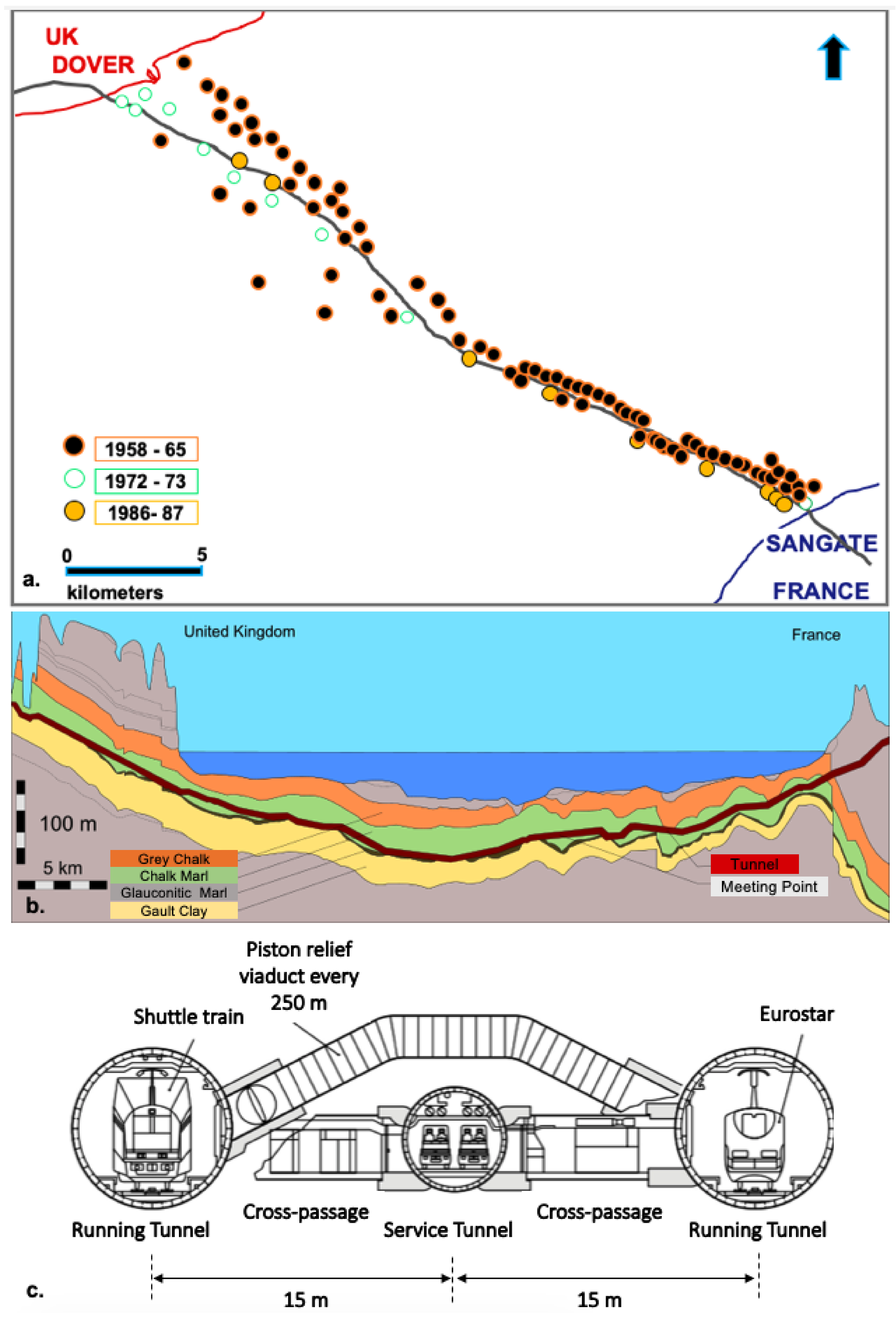
Many geotechnical investigation campaigns took place in the Channel route during a 100-year period. It should be noted that the area between Dove and Sangatte (Figure 5a) is one of the most detailed investigated areas throughout the history. In total, 116 marine and 70 land boreholes drilled and 4000 km of geophysical surveys took place [41]. On average, boreholes were drilled per 1 km of the route under the clearly identified geological conditions. In areas with a complex geological structure including faulting, folding and in the absence of outcrops on land, deeper boreholes were drilled reaching the depth of the tunnel [41]. Deep boreholes were drilled mainly in areas were unfavourable geological conditions were observed. On average, deep exploration boreholes were drilled on the selected route of the Channel tunnel. Down-the-hole logging methods were performed in several of the boreholes drilled in the Channel. In situ testing performed included Verticality (inclinometer) tests, Calliper tests and Packer permeability tests [41].

The geotechnical investigations campaigns are shown in

Table 2. Boreholes drilled in every Ground Investigation (GI) Campaign [42].

GI Campaign		UK Land Boreholes	UK Offshore Boreholes	French Offshore Boreholes	French Land Boreholes
1958–1959	early marine borehole	3	5	3	1
1962–1965	marine borehole	14	32	41	10
1972–1974		8	9	7	-
1986–1987 (Phase I)	site investigation	19	3	9	15
1988 (Phase II)		-	5	2	-

. Four geophysical survey campaigns were also conducted during each period. Seismic profiling produced between 1958 and 1959. Additional surveys were performed in 1964–1965 and in 1972.

In 1974 the excavation of a 2 km pilot tunnel in Shakespeare Cliff was planned to be part of the service tunnel. The project aimed to provide data for the performance of the tunnelling machine and the construction methods that would be used. Unfortunately, the project was aborted, but not before 290 m of access tunnel, 490 m of conveyor adit, 110 m of marshalling tunnel and 260 m of long service tunnel were excavated [42]. Two large channels infilled of alluvium were also recorded. In Dover, a highly weathered area was investigated. The new era of investigations started in 1986–1988, with the then most updated technology. The last campaign of 1986–1988 improved the already existing data focusing on specific areas of interest such as the top of the Gault Clay, the thickness and permeability of Chalk Marl and its weathering grade. This campaign consists of two exploration phases. Phase I exploration with seismic methods determined the geology at depths between 150 m to 800 m below sea bed. Phase II targeted possible faulted areas [43]. In Phase II, a seven-borehole program took place in order to minimise the risk in areas of high uncertainty such as Fosse Dangeard, an ancient valley infilled with sediments reaching depths of 80 m below the sea-bed [42].

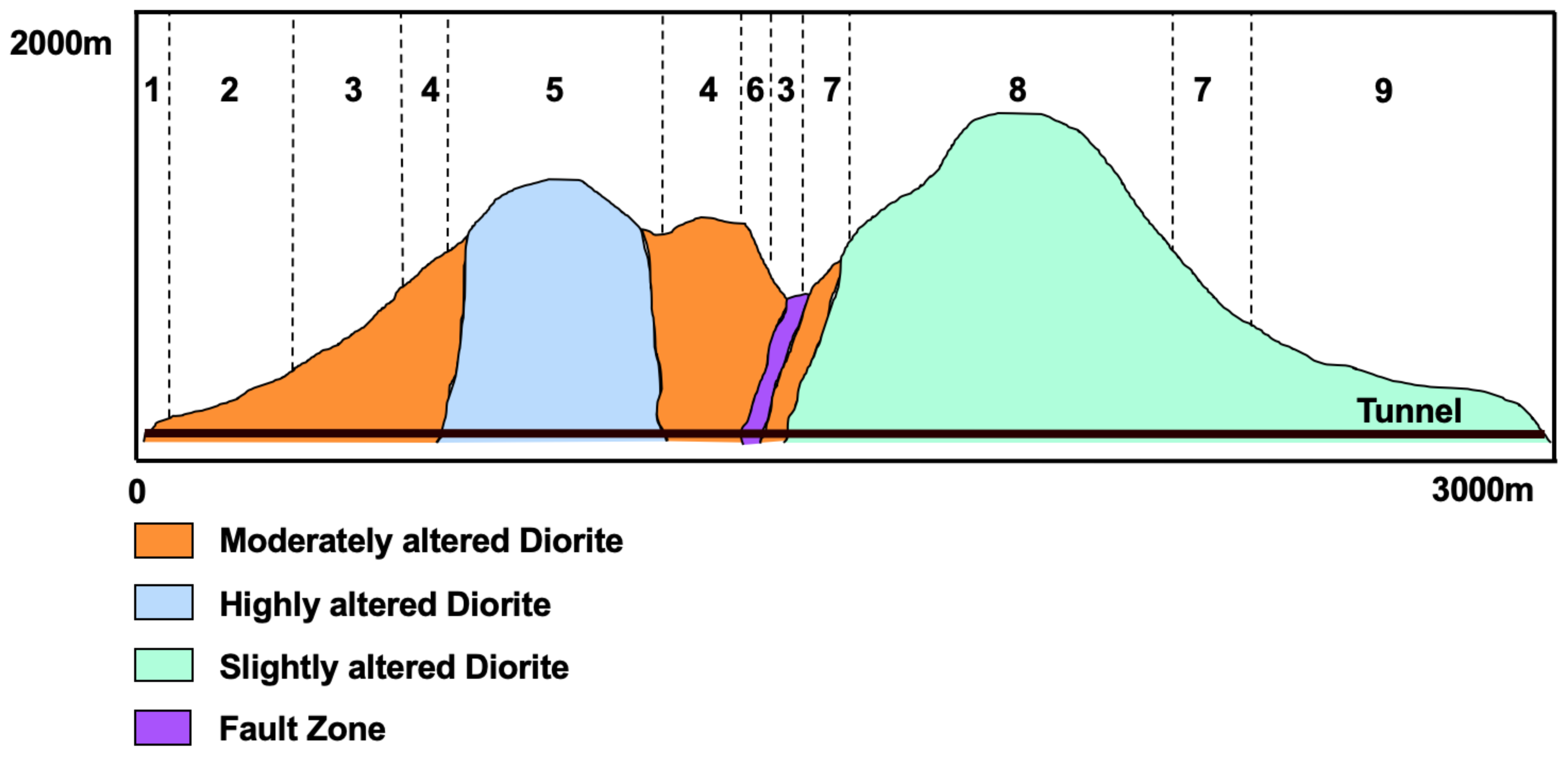
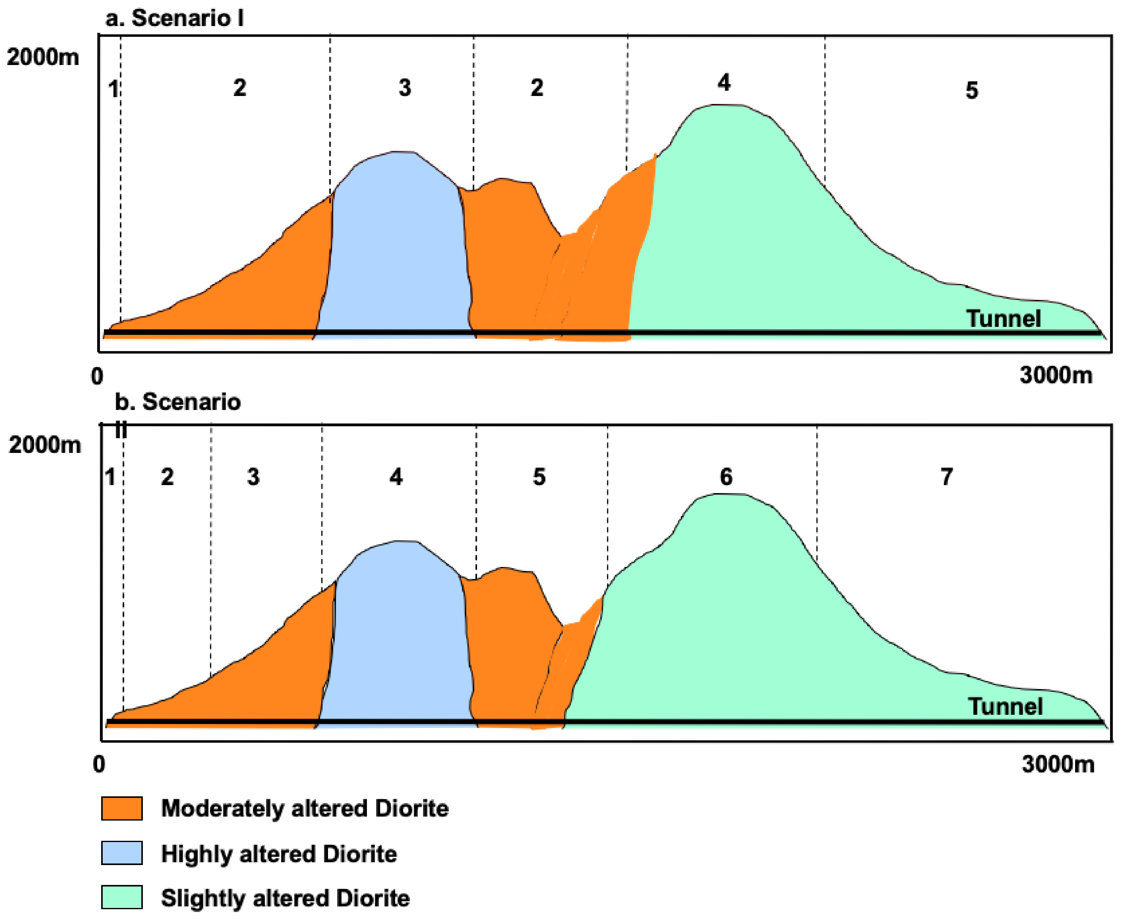
According to the authors of reference [38], three major lithostratigraphic units were identified (Figure 5b):

• The Gault Clay: weak clayey calcareous mudstone susceptible to softening and swelling.
• The Glauconitic Marl: due to the sharp contact the unit was easily identified from the underline unit.
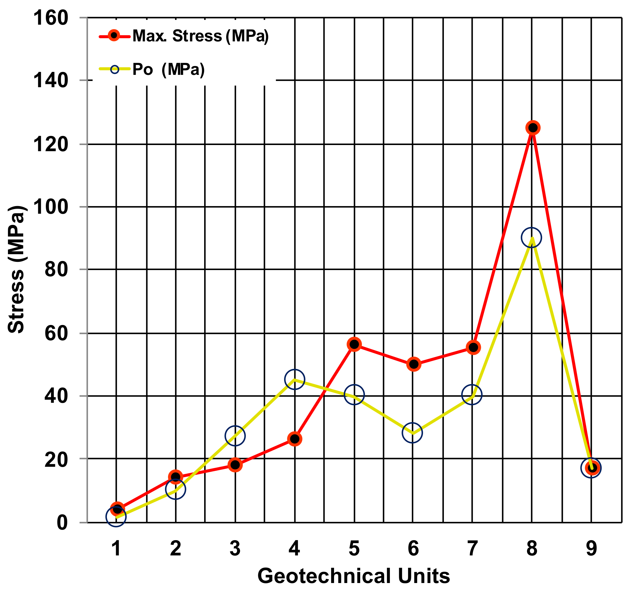
• The Chalk Marl: a weak grey calcareous mudstone. Chalk Marl was cyclically bedded with material varying from moderately strong (UCS < 50 MPa) in the sponge beds to weak (UCS < 5 MPa) in clay-rich layers. The overlaying Grey Chalk had similar cycles of carbonate-rich and clay-rich beds.

It should be stated that the tunnel was excavated mainly in the Chalk Marl formation. Ground investigations for the Channel tunnel have a long history, and therefore, most of the geological factors were investigated in detail during the various ground investigation campaigns, but especially the last campaign. Despite this extensive work, the Tunnel Boring Machines (TBMs) still ran into adverse, wet and blocky ground, shortly after the Marine Service Tunnel (MST) had commenced. The tunnel design (Figure 5c) was set up for essentially ’dry conditions’, whereas localised discrete sections of wet, faulted and broken ground was only anticipated on 5% of the total drive length. This required major changes in the design of the TBM system [44]. More specifically, water inflow was one of the major problems during the tunnel construction. Waterflow ranged from 0 to 100 L/m. Most of the problems faced between 19 to 23 km, with the vicinity of this area recording an inflow of around 20 L/m. Grouting proved a very successful tactic, eliminating the problem in most of the cases. In addition to the water inflows, water salinity (chloride concentrations) was encountered in the face tunnel, mainly in the running tunnels. The importance of high salinity water lies on the effect of lowering the volume of Marl Chalk and was encountered between 20 to 23 km. Shrinkage could lead in reducing of the in-situ stress and end up in opening the discontinuities [45]. The areas where the most adverse ground conditions encountered were from chainage 20.28 to 23.75 km and the area with chainage from 27.3 to 28.4 km, respectively. In the first area, extensive faulting was present, while in the second, water inflow and overbreak due to the Glauconitic Marl presence was encountered. An anticlinal structure bounded by faults was also recorded from 28.2 to 28.4 km.

In conclusion, according to [46], the investigations:

• Substantially underestimated the length of tunnel which was subject to overbreak.
• Did not identify those areas where significant overbreak occurred.
• Did not identify the area of consistently high-water inflow between 20 and 24 km, especially in the vicinity of 23 km.
• Did not identify the various structural zones along the tunnel route.
• Did not identify the effect of minor folding on tunnel stability.

3.2. Data Collection

The dataset developed and further analysed herein have been based on published available data. More specifically, the following key references have been used are shown in

Table 3. Key references used to develop a database.

Reference	Year	Author
Managing a Mega-project: The Channel Tunnel	1990	[48]
Managing large-scale technology and inter-organisational relations: The case of the Channel Tunnel	1997	[49]
The Financing and Financial Results of Eurotunnel: Retrospect and Prospect	2000	[50]
The Channel Tunnel—an ex post economic evaluation	2006	[51]
Review of Eurotunnel’s Decision-Making Process	2007	[52]
The hold-up problem in the management of construction projects: A case study of the Channel Tunnel	2007	[53]

.

In the above publications, detailed cost and cost breakdown figures for several periods of the Channel tunnel project are presented from the tender phase until the end of construction and during the operation period. In most of the cases, these cost figures are not identical but similar. It should be noted that mainly data presented by [49] was chosen, since the cost breakdown presented was the most detailed with cost figures taken from pre-construction period (1978) to mid-construction (1990) followed by the end of construction in 1994 until 1998, the fourth year of operation. The summarised financial data was taken from Eurotunnel Rights Issue Document report [52], as this source was considered the most reliable.

It should also be noted that the geological geotechnical data (i.e., geology, ground investigation campaigns, history, unforeseen ground conditions and construction methods) were taken from data presented by reference [46].

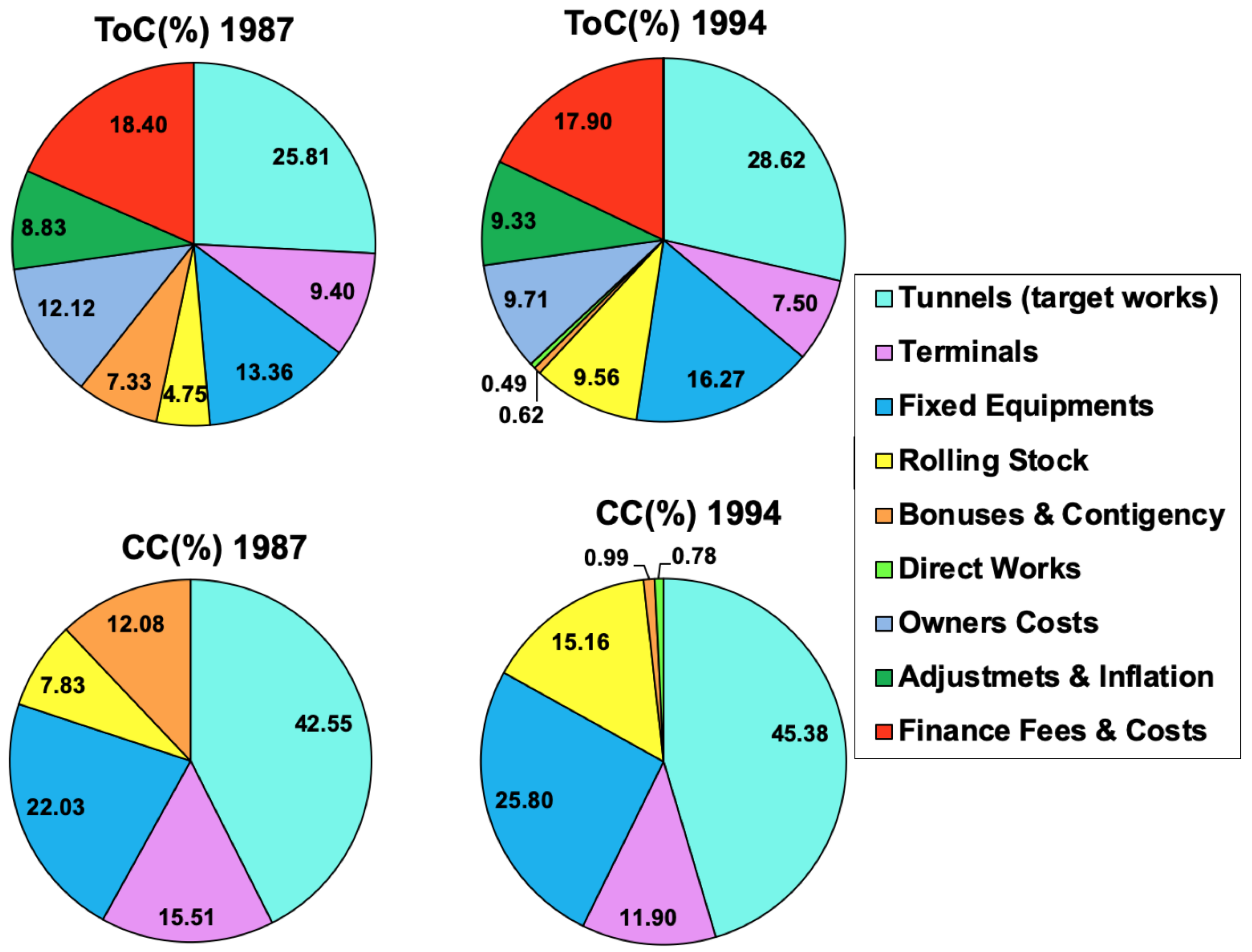
For the purpose of this research, three types of cost are used and analysed: The Tunnel Cost, the Construction Cost and the Total Cost.

• Tunnel Cost (TuC) includes the Target Works cost that covers all tunnelling and related equipment costs including the tunnel boring machines expenditure.
• Construction Cost (CC) covers the tunnel cost (TuC), the terminals, rolling stock, bonuses/contingency and the direct cost.
• Total Cost (ToC) covers the construction cost (CC) plus the finance related cost, owners cost, finance fees, capital expenditure, net cash flow, inflation and interest reserves.

Detailed cost figures are available for four calendar years: 1987, 1991, 1994 and 1998.

• The first, dating from 1987, is the pre-construction cost based on the tender in 1985. This cost is considered an estimate, as in most cases it is a representative percentage of the total cost (ToC) due to the shortage of information and data available at the preliminary design stages. The latter is more evident in tunnelling projects where the uncertainty of the geological medium is the most significant factor that leads in significant deviations from the total cost.
• The second cost figure, dating from 1991, is based on the mid-construction year. During this year, the last ground investigation was already conducted along with a considerable percentage of the tunnel construction, in other words cost overruns were running already at this stage of the project. An example of cost overrun for the tunnel construction can be found in the following (Equation (2)):

  $$\mathit{Cost} {\mathit{overrun}}_{ \mathit{during}\mathit{Tunnel} \mathit{Construction}}(\%)=\raisebox{1ex}{$\left(cost in 1987\times 100\right)$}\!\left/ \!\raisebox{-1ex}{$\left(cost in 1991\right)$}\right.$$

  (2)
• The third cost figure dates from 1994, during which the construction was finished and the project was operational while the tunnelling cost and construction costs figures were considered to be the final. An example of cost overrun for the total construction can be found in the following (Equation (3)):

  $$\mathit{Cost} {\mathit{overrun}}_{ \mathit{for} \mathit{the} \mathit{Total} \mathit{Construction}}(\%)=\raisebox{1ex}{$\left(cost in 1987 \times 100\right)$}\!\left/ \!\raisebox{-1ex}{$\left(cost in 1994\right)$}\right.$$

  (3)

In 1998, after four years of the project’s operation, the final cost overrun revealed. An example of cost overrun for the project can be found in the following (Equation (4)):

$$\mathit{Cost} {\mathit{overrun}}_{ \mathit{final}} (\%)=\raisebox{1ex}{$\left(cost in 1987 \times 100\right) $}\!\left/ \!\raisebox{-1ex}{$\left(cost in 1998\right)$}\right.$$

(4)

Pricing figures for these four calendar years were adjusted and revised to 2019 values as described extensively below. The revision to 2019 price figures contributes towards a more realistic comparison under a common reference year (i.e., 2019). The methodology used in this analysis is based on the Case Based Reasoning (CBR) Method. CBR is formed in experience gained by cases, data and information of the past. In this method, it is important to find accurate and precise similarities between a new case and an older one [54].

Calculating of Inflation Rate and Cost Adjustment in 2019 Price

The cost revision to 2019 pricing also involved calculating effect of inflation. For this purpose, the inflation estimation was made based on the Bank of England estimator. A formula (Equation (5)) is provided below showing how pricing in 1987 is revised and adjusted to 2019 figures. It should be stated that the cost cannot be adjusted to the 2020 price, since the inflation rate is not yet finalised for the current year.

$${\mathit{Cost}}_{\mathit{revised}} \mathit{in} 2019 = {\mathit{Cost}}_{\mathit{initial}}\mathit{in}1987x\left(\raisebox{1ex}{$2019 price index $}\!\left/ \!\raisebox{-1ex}{$1987 price index$}\right.\right)$$

(5)

Equation (5) is applicable for costs ranging from £1 to £1 trillion. Equation (6) calculates the Average Inflation (AI) rate between two years (i.e., 1987 and 2019) and takes into consideration deflation as a negative inflation, which can imply that comparisons of price further back in time and over long periods are less accurate than comparisons over short periods in recent years. The average (annual) inflation from 1987 to 2019 was estimated as 3.3% [55]:

$$AI =\left({\left.\left(\frac{2019 price index}{1987 price index}\right.\right)}^{0.1}-1\right)*100$$

(6)

3.3. Cost Analysis

In this section primarily the data from: (a) reference [49] is used as released from the Eurotunnel for the period from 1987 to 1998 (

Table 4. Channel tunnel project costs (initial data from: [49]; [44], apart from % change).

Cost (in mGBP)	1987	1990	1994	1998	% Change (1987–1998)
Exploration 4th campaign	17
Exploration overall (estimated)	80
Construction and equipment
Tunnel Cost (target works)	1814	2836	3212	3212	77
Terminals	661	763	842	842	27
Fixed equipment	939	1223	1826	1826	94
Rolling stock	334	823	1073	1073	221
Bonuses and contingency	515	98	70	70	−86
Direct works			55	55
Total construction	4263	5743	7078	7078	66
Finance related cost
Owners costs	852	700	1090	1128	32
Adjustments and inflation	621	1178	1047	1146	85
Finance fees and costs	1293	1584	2009	4757	268
Capital expenditure				222
Net cash flow		224		1859
Transfer and interest reserves				72
Total financing cost	2766	3686	4146	5466	97
Total Cost	7029	9429	11,224	12,554	78

) and (b) reference [44], regarding the English and French TBM performance shown in

Table 5. Tunnel Boring Machine (TBM) performance for: a. the French side and b. the English side [44].

a. French side
	Sea			Land
TBM name	STM	RTNM	RTSM	STL	RTNL	RTSL
Cutter head diameter (m)	5.77	8.78	8.78	5.61	8.64	8.64
Driven distance (m)	15,528	19,920	18,769	3162	3174	3176
Volume (m3)	405,823	1,205,447	1,135,795	78,119	185,996	186,113
b. English side
	Sea			Land
TBM name	MST	MRTN	MRTS	LST	LRTN	LRTS
Cutter head diameter (m)	5.38	8.36	8.36	5.76	8.72	8.72
Driven distance (m)	21,770	17,651	18,803	7930	7911	7859
Volume (m3)	494,644	968,393	1,031,595	206,532	472,209	469,105

.

The above data have been further investigated in detail and the following parameters are analysed:

• Cost per tunnel diameter.
• Cost per excavated distance/length (m).
• Cost per cubic meter of excavated material.
• Excavation method as a percentage of the total excavated length.
• Total cost overrun.
• Construction cost overrun.
• Tunnelling cost overrun.
• Cost overrun adjusted to the 2019 price.
• Tunnelling cost as a percentage of the total cost and construction cost.
• Ground investigation cost as a percentage of the total cost, construction cost and tunnelling cost both for pre-construction and final price.
• Estimation of the impact of higher expenditure of ground investigation in the total cost and in the tunnelling cost, respectively.

These parameters provide a good understanding for the project and in combination with the previous geological investigation campaigns, add value in developing a further understanding on what could have been improved in the planning and execution of this complex project.

In total, 12 TBMs were used to excavate both the English and the French side of the Channel tunnel. The English TBMs excavated 81,924 m, while the French TBMs excavated 63,729 m. In addition to the mechanised excavation methods, conventional methods were used. New Austrian Tunnelling Method (NATM) was used in both sides of the tunnel with the English excavating 2716 m. Approximately the same length was excavated by the French using NATM method. For both sides of the tunnel, multiple TBM diameters were used, ranging from 5.38 m to 8.78 m (Table 5). The average excavated diameter is 7.59 m. In total, more than 8,167,243 m³ of material had been excavated from both sides of the Channel tunnel, as shown in

Table 6. Construction Methods and Cost Figures for the Channel tunnel (initial data taken from: [45], apart from 2019).

TBM and New Austrian Tunnelling Method (NATM) Details
Excavation Method	Distance (m)	% from Total Excavated Length
British TBM	81,924
French TBM	63,729
Overall TBM distance	145,653	96.542
NATM British side	2716
NATM French side	2500
NATM total	5216	3.457
Overall	150,869
Volume of excavated material
Excavation Method	Volume (m3)
French TBM	3,197,293
British TBM	3,642,478
TBM total	6,839,771
NATM French side	636,250
NATM British side	691,222
NATM total	1,327,472
French side total excavation	3,833,543
British side total excavation	4,333,700
Volume total	8,167,243
Cost per cubic meter of excavated material
Excavation Cost	£
Cost per meter in 1994 price	22,052
Cost per meter in 2019 price	43,500
Cost per cubic meter in 1994 price	393
Cost per cubic meter in 2019 price	776

.

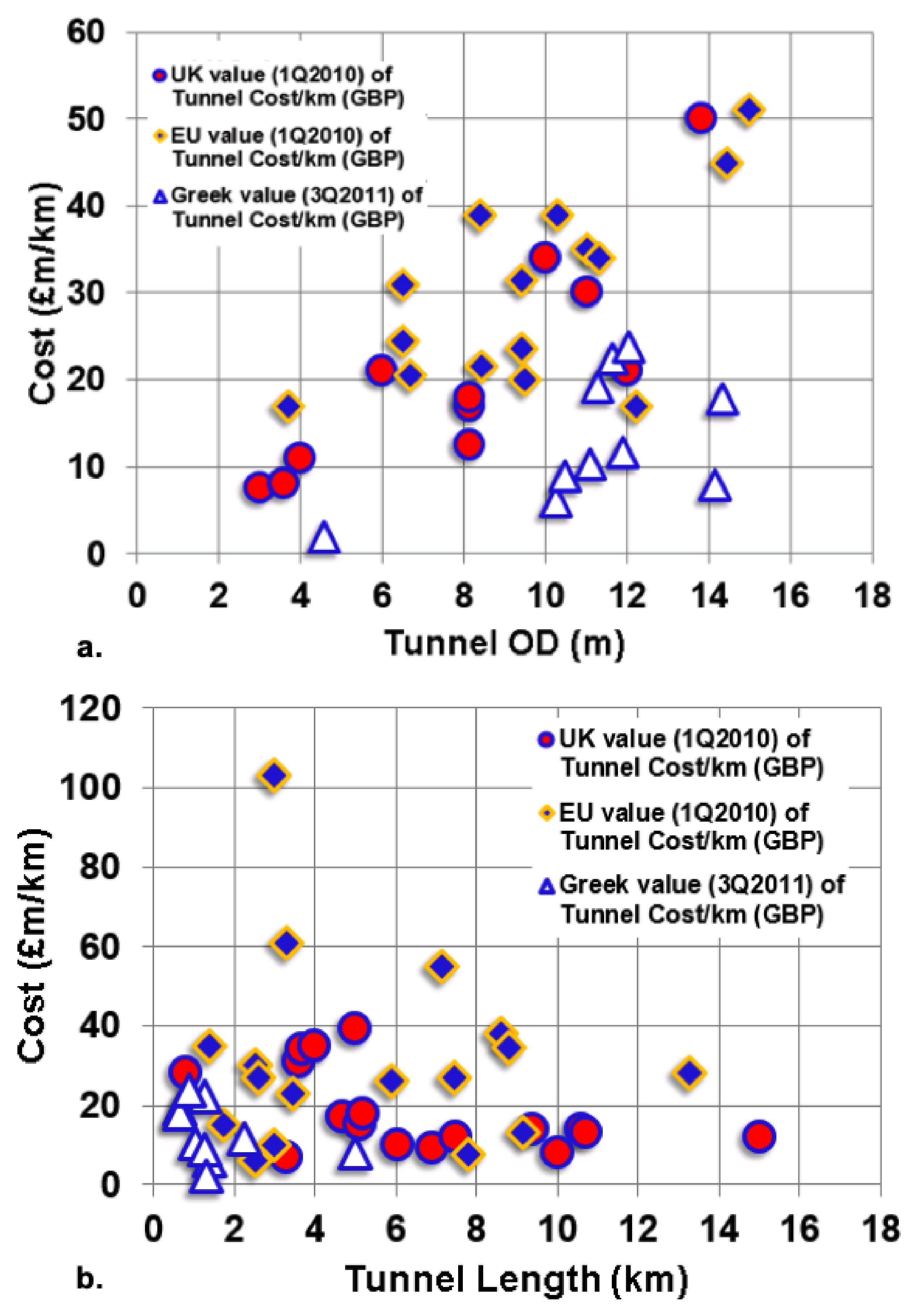
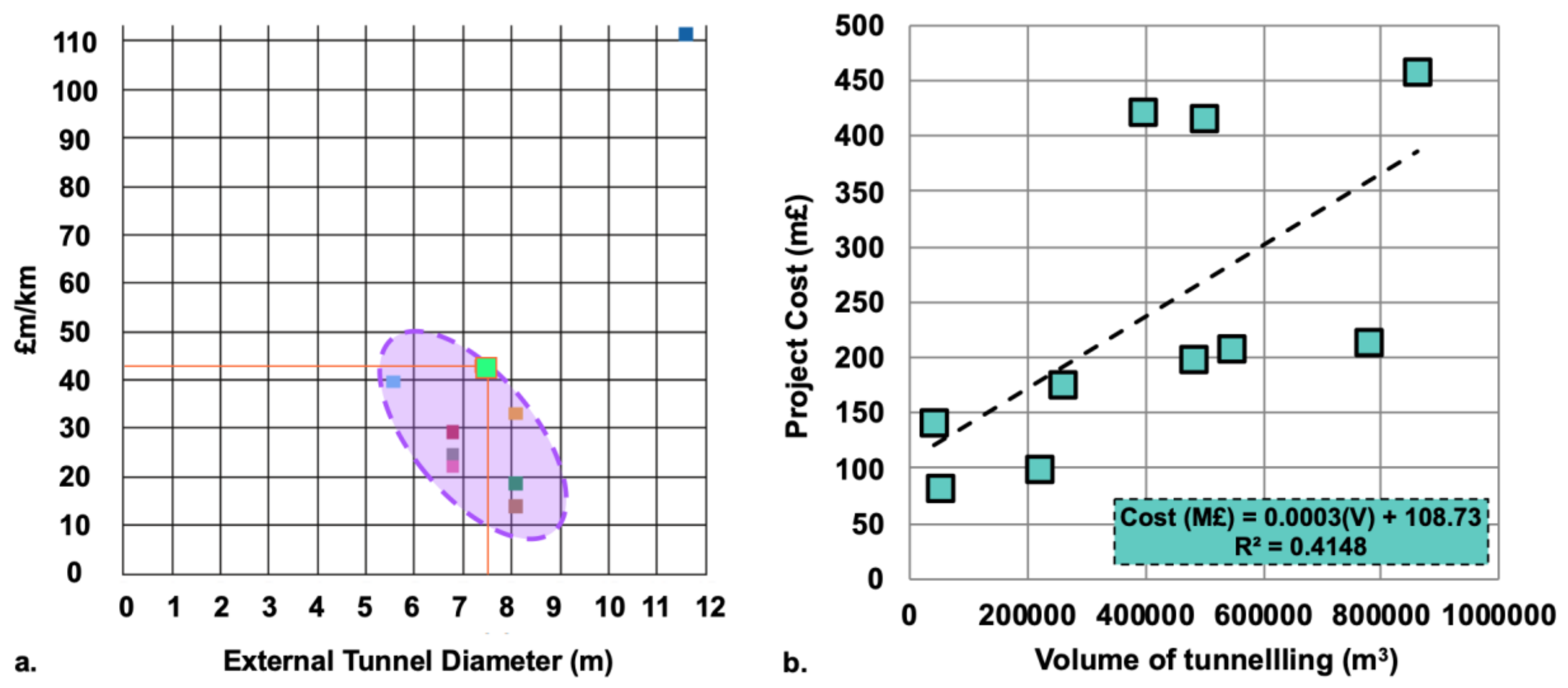
The cost per meter of excavation converted to the 1994 price is £22,052. The average diameter, combining the British and French tunnels, was 7.59 m. After converting this cost to the 2019 price and taking into consideration an average inflation of 3.3% [54], this amount becomes 43,500 £/m. Compared to the price provided in the literature for other tunnels constructed in the UK (from Case Study: Benchmarking tunnelling costs and production rates in the UK, 2018), the Channel tunnel is more expensive. The average Construction Cost (CC) per tunnel length in the UK is estimated at 32,000 £/m, which is still within the typical range based on published data by the Project Authority shown in Figure 6a.

The cost per cubic meter of excavated material for this case is estimated at £393.2 as per 1994 and £775.6 as per 2019 (Table 6). Other tunnels constructed in the UK (Case study: Benchmarking tunnelling cost and production rates in the UK) have a cost that ranges from £274 to £3525 per m³ (Figure 6b). Although the cost of excavation per cubic meter has a wide range of values, the Channel tunnel lies in the lower bound of this list. This correlation has a significant limitation, since the comparable projects have a notably lower size than the Channel tunnel project.

According to reference [56], the NATM method was used in several occasions: in the Shakespeare Underground development, Castle Hill tunnels and UK Crossover, along with other auxiliary works such as pump stations, cross passages, drainage tunnels etc. Thousands of meters were excavated using the NATM method, but the most important was in the Shakespeare Underground development, which served as the-starting point of the tunnel boring machines with a length of 2716 m of tunnels and adits and an additional 2500 m for the French side. 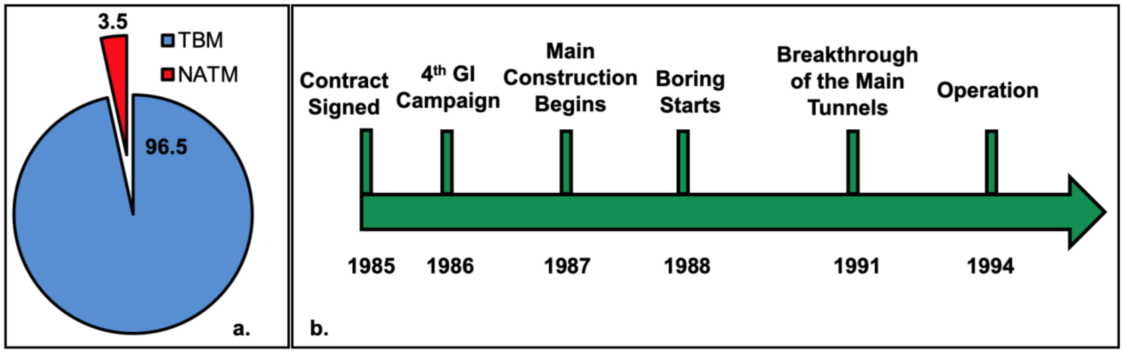Figure 7a shows that the 96.5% of the tunnel construction was made with TBM, while the rest was completed with the NATM method.

Cost figures from Table 4 are used to calculate the cost overrun. At this point, it should be noted that the 1987 cost figures are referring to the pre-construction cost as calculated for the tender phase and before the completion of the last ground investigation campaign (1986–1988), while the construction of the tunnels started in 1988 and the project became operational in 1994. The timeline of the project with the important dates is summarised in Figure 7b.

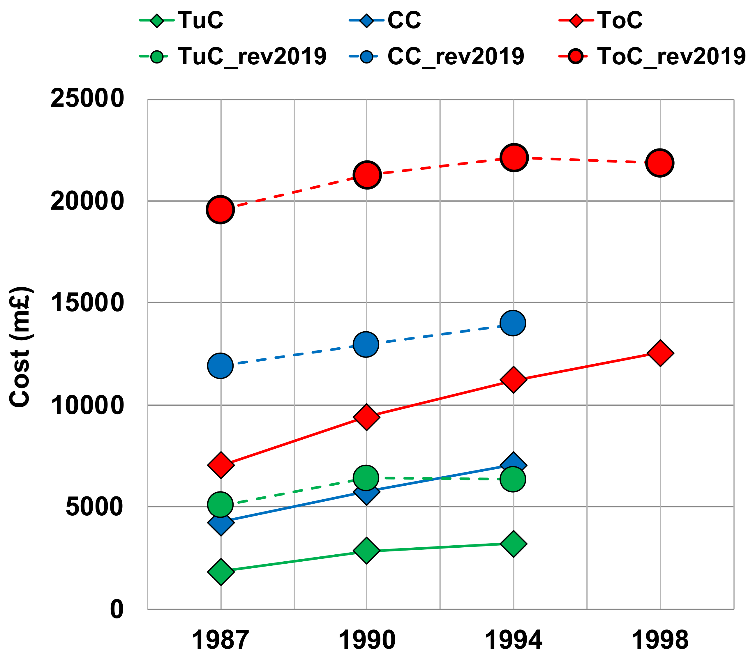
The Tunnel Construction (TuC) cost is calculated for the period from 1987 to 1994 including the period from tender to completion and operation of the project. For the Total Cost (ToC) of the project, a longer period was required for the overrun calculation since the financial data includes the period from 1994 to 1998, where capital expenditure, finance fees and owner’s costs are taken into consideration. The ToC overrun is calculated at 78%, the CC overrun at 66% and the TuC overrun at 77%, as presented in Table 4 and shown in Figure 8. These cost overruns provided an overall notion about the cost of the project. A major part of the overrun is due to the inflation from year to year that raise the cost of the project in an excessive amount. In order to get a better understanding about the “net” cost overrun of the project, the cost figures are adjusted to 2019 price units and the cost overrun are calculated as shown in

Table 7. Cost overrun adjusted to recent (2019) price units.

Cost in m£	1987_rev 2019	1990_rev 2019	1994_rev 2019	1998_rev 2019	Cost Overrun (%)
Total Cost (ToC)	19,608	21,254	22,140	21,891	13
Construction Cost (CC)	11,892	12,945	13,962	5	17
Tunnel Cost (TuC)	5060	6393	6336	6	26

.

The revised ToC overrun plunges to 13%, while the CC overruns at 17% and the TuC at 26%. The cost overruns and the way the cost escalates throughout the years is provided in Figure 8 (dashed lines). It is important to mention that the ToC cost and the TuC adjustment are made only for the period from 1987 to 1994, since after the completion of the construction these figures did not change in contrast to the overall cost, which continued increasing up to 1998.

In Figure 9, the TuC is presented as a percentage of the CC and the ToC and it considers both the tender and final costs (1987 and 1994). It is evident that the tunnelling cost increased by almost 3%, both as part of the overall cost and the construction cost after the completion of the project. This is almost £1.4 billion (cost overrun from 1987 to 1994) due to the unforeseen ground conditions. Furthermore, regarding the amount spent on ground investigation, the cost was £17 million as per reference [38], previously presented in Table 4. It should be noted that this amount represents only the fourth and final ground investigation campaign. No detailed cost figures were found for the cost of the previous ground investigation campaigns, but an estimation was made based on the data available, which calculates the overall ground investigation campaigns cost to be around £80 million. This amount results from the estimation that each marine borehole costs £0.5 million and each land borehole costs £20,000 based on the 1987 price. For the geophysical surveys, an additional £20 million is estimated to be part of the ToC.

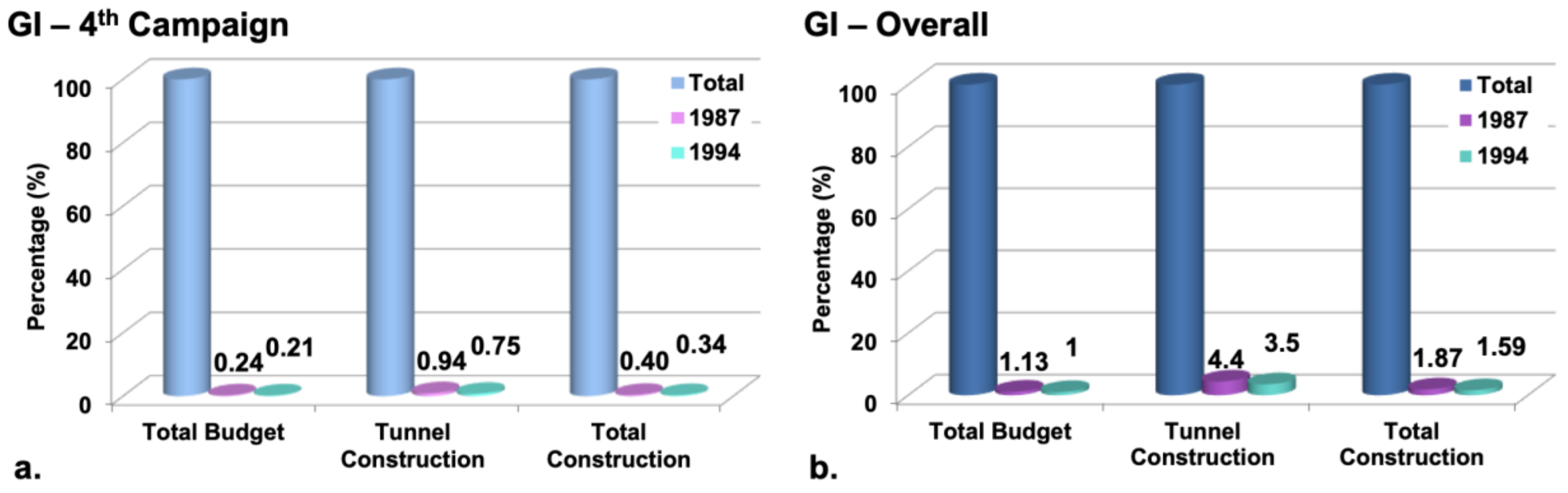
As a percentage of the tunnel construction, the fourth ground investigation accounts for 0.94%, more specifically, it is 0.4% of the ToC and 0.24% of the overall budget (Figure 10a). The aforementioned rates are calculated as a percentage of the cost of the tender price in 1987. For the 1994 price, these rates become even lower with the ground investigation, covering 0.75% of the TuC, 0.34% of the ToC and 0.21% of the overall project cost (Figure 10a). As for the overall ground investigation expenditure, this covers 1.13%, 1.87% and 4.4% of the final CC, ToC and TuC, respectively, with the 1987 price (Figure 10b). For the 1994 price, these percentages decrease to 1%, 1.59% and 3.5%, respectively (Figure 10b). No calculation was made for the final price of 1998 since the construction had finished in 1994.

In regards to the impact that a higher expenditure would cause to the cost of the project, the analysis was based on Clayton’s data [57]. In his research, results derived from 51 case studies articulate that cost overruns are common even in areas with uniform geological conditions. This is despite the fact that in most of the cases, the ground investigation is conducted by both consultants and contractors who are familiar with the area of the project and are able to obtain any information potentially needed. Clayton [57] highlights the fact that designers and contractors never or seldom exploit the geological investigation possibilities, failing thus to produce a sound geological model which leads to unsound tunnel designs and ultimately to cost overruns. Ground investigations expenditure typically covers 1% or even less of the total project cost in the case studies analysed. These percentages, according to reference [57], lead to overruns of more than 77%. 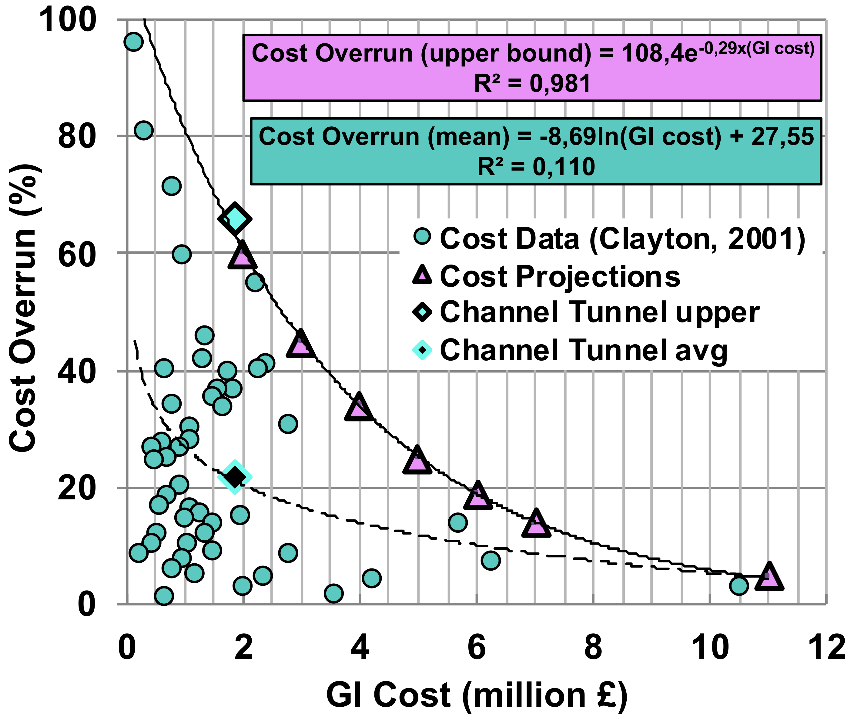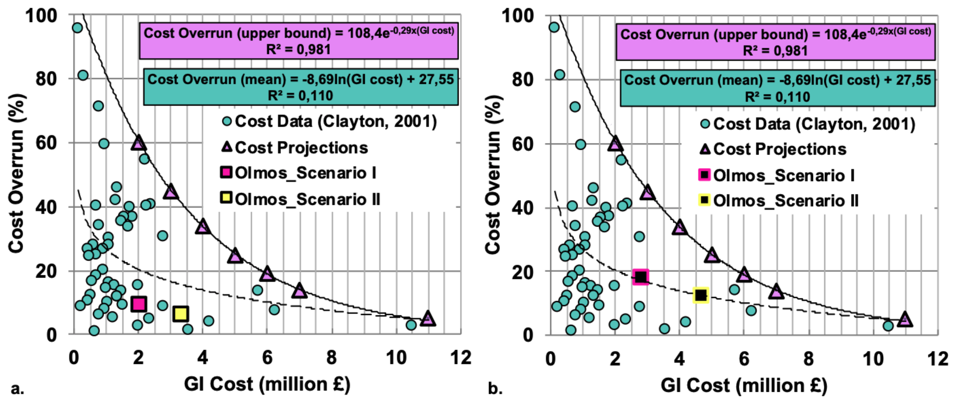Figure 11 shows that an optimum expenditure allocated to Ground Investigation (GI) ranges between 5–6% of the total budget and contributes to achieving an overall cost overrun of less than 10%. In the Channel tunnel case, the ToC overrun is estimated to be 66%, shown in Figure 11, in which the GI is only 1.87% in the tender process as previously observed. The upper bound of the cost overrun is shown in Figure 11. The case study of Channel tunnel lies on this line with 66% overrun in the ToC. The best fit for the mean trend of this population can be expressed with a logarithmic equation (Equation (7)):

Cost overrun = −8.69ln(GI cost) + 27.55

(7)

In this trend line, it is also observed that for an expenditure of 1.87% the average cost overrun is 22%. While the upper bound line can be expressed with the (Equation (8)):

Cost overrun = 108.4e^{−0.29(GI cost)}

(8)

The projection of this trend line provides also an estimation of the overruns with higher expenditure on GI based on Clayton’s case studies. Consequently, the Channel tunnel project has a cost overrun above the average trend recorded.

In

Table 8. Estimation of overruns of the project cost with floating expenditure in ground investigation.

Ground Investigation Expenditure (%)	Construction Cost Overrun Estimation (%)	Construction Cost Overrun (2019 Price in Million £)
1.87	66	7849
2	60	7135
3	45	5351
4	34	4043
5	25	2973
6	18	2140
7	14	1665
11	8	951

, an estimation of how the additional expenditure in GI would have impacted the CC is presented along with the actual figures of overruns. It is inferred that more than 11% of GI would lead to no difference in the cost overrun.

4. Olmos Tunnel

In the second case study, a 3 km section of the Olmos tunnel was analysed and the calculated CC is compared against scenarios with different levels of detail in the site investigation. The design of the Olmos Transandean Tunnel was initially conceived in the 19th century and it is part of a larger water transfer project. While the site investigation work commenced in 1980s, the recent construction began in 2003. Drill and blast operations were performed mainly in the eastern segment of the tunnel, but the biggest part was excavated with TBM. Breakthrough of the tunnel took place in December 2011 after transecting metamorphic schists as well deformed andesites and diorites, porphyry and tuff complexes with a maximum cover of 2500 m [58]. In this case study, the as-built cost of the tunnel was calculated based on the cost values taken from Spon’s Civil Engineering Book and Highways Works Price Book [1] in GBP in 2019 pricing figures. Two separate cases with different levels of site investigation were analysed, and the cost overrun for each is calculated and compared. The tunnel conditions were examined with the use of RS2 and Unwedge [59] in order to identify the failure modes and determine the support measures. The final cost of the support measures was calculated based on the prices taken from Spon’s book [1].

4.1. Rock Parameters and Numerical Modelling

In this analysis, as-built data from [11] were used. In the section of the Olmos tunnel, nine domains (geotechnical units) were identified based on the in-situ stress ratio (k₀). The geology consists mainly of diorite with different levels of alterations and a fault zone approximately in the middle of the tunnel length (Figure 12).

Intact rock strength and the joint strength parameters were used for the identification of the failure modes and the calculation of the temporary support measures. The tunnel diameter is 10 m with horseshoe geometry and the excavation method is assumed to be Drill and Blast in diorite rock. No ground water conditions were taken into consideration for the calculations. Stress two-dimensional (2D) analysis was undertaken using the RS2 software and wedge failures with Unwedge 4.0 software [59]. For the stress analysis, the generalised Hoek-Brown failure criterion was considered, which is applicable to rock mass with more than three discontinuity sets. Materials are analysed as plastic, behave elastically until they reach their peak strength and deform plastically past it. Boundary displacements are zero in all cases examined, at a distance less than four times the excavation diameter. Top boundaries were free of restrains. All boundaries are set at 36 m from the centre of the excavation (Figure 13). One limitation of the stress analysis is that only three joint sets can be considered in the RS2 software calculations.

According to reference [11], the anticipated failure modes based on this tunnelling environment are:

• (R) Ravelling: progressive gravity driven failure under low confinement conditions of a blocky/disturbed/seamy to disintegrated rockmass [60].
• (W) Wedge: for blocky rockmasses, structurally controlled gravity driven failure of individual blocks or wedges under low confinement.
• (T) Stress triggered structural failure: localised material or structural yield around the tunnel excavation caused by the induced stress allows for the subsequent release of blocks or wedges under gravity loading.
• (U) Rock fracture: in blocky to intact hard rock rockmasses, stress driven fracturing and structural failure fractures the rockmass into small fragments. Failure in massive rockmasses is typically directionally controlled by the in-situ stress condition (both in terms of magnitude and ratio), whereas in blocky rockmasses, failure surrounds the entire tunnel excavation. Rockmass behaviours include slabbing, spalling and rock or strain bursting.
• (Q) Rockmass shearing and squeezing: occurs in overstressed rockmasses where material and structural shear and tensile failure surround the tunnel excavation. Rockmass shearing is typically characterised by medium strains (1–2.5%), whereas squeezing typically encounters strains > 2.5% [18,61].
• (H) Structurally controlled shearing: in very blocky to blocky rockmasses, stress driven material shear failure is structurally controlled by the rockmass discontinuities.

Table 9. Geotechnical parameters for: a. intact rock and b. joint [11].

a. Intact Rock
Domain	UCS (intact)	Depth (m)	Geological Strength Index (GSI)	mi	Ei (MPa)	v (Poisson’s Retio)	φpeak (o)	φresidual (o)	c(Peak) (MPa)	c (Residual) (MPa)	σt (Peak) (MPa)	σt (Residual) (MPa)	k0	σV	σh
1	50	0–50	25–35	25	13,000	0.3	38	24	10	6	5	0	1	1.4	1.4
2	50	50–300	35–45	25	13,000	0.3	38	24	10	6	5	0	1.2	8	10
3	75	300–700	50–70	25	13,000	0.3	38	24	10	6	5	0	1.4	20	27
4	150	700–1000	40–65	25	13,000	0.3	38	24	10	6	5	0	1.6	28	45
5	100	900–1200	60–70	25	24,400	0.3	42	28	14	8	6	0	1.2	34	40
6	150	700–1000	15–25	25	13,000	0.3	38	24	10	6	5	0	0.9	28	25
7	100	500–900	65–80	25	13,000	0.3	38	24	10	6	5	0	1.6	25	40
8	150	900–1600	75–85	25	48,800	0.3	47	33	19	12	8	0	2	45	90
9	150	50–500	60–70	25	48,800	0.3	47	33	19	12	8	0	1.2	14	17
b. Joint Sets
Domain	GSI	φpeak (o)	φresidual (o)	c (Peak) (MPa)	c (Residual) (MPa)	σt (Peak) (MPa)	σt (Residual) (MPa)	Joint Sets	Spacing (m)	Inclination		Length (m)		Length of Section (m)
1	25–35	36	31	0.5	0	0.05	0	5	0.3,0.4,2	−60, 10, −31, 54, −54		10		91
2	35–45	36	31	0.5	0	0.05	0	4	0.6,4	22, −54, 40, −75		10		236
3	50–70	44	37	0.7	0	0.07	0	3	0.8,1	−54, 40, −10		10		218
4	40–65	40	34	0.6	0	0.06	0	4	0.6,4	22, −54, 40, −75		10		273
5	60–70	44	37	0.7	0	0.07	0	3	0.8,1	−54, 40, 10		4		509
6	15–25	28	25	0.3	0	0.03	0	5	0.2	22, 50, 80, −30, −54		4		55
7	65–80	48	40	0.8	0	0.08	0	2	1, (0.1)	55, −45		4		273
8	75–85	54	40	1.2	0	0.12	0	2	2, (0.1)	45, −45		4		709
9	60–70	44	37	0.7	0	0.07	0	3	0.8,1	−54, 40, −10		4		636

presents the intact rock and the joint strength parameters used for thenumerical analysis as taken from the as-built data [11].

4.1.1. Numerical Analysis

The nine domains (Geotechnical Units) were analysed, and the results are shown in Figure 14 and Figure 15. As already stated, a maximum of three joint sets were used due to the limited computing power; for this reason, the predominant joint sets were chosen for the modelling analysis.

Geotechnical Unit 1: No significant displacements are observed in this domain, and maximum displacement is below 1 mm at the floor of the tunnel. In addition, the joint strength is higher than the stresses, thus there is no significant number of failed joints, whereas the maximum stresses around the excavation are 4 MPa. No yielded element or plastic zone is formed, as the strength of the material in this case is higher than the in situ stress.

Geotechnical Unit 2: For the second domain of the tunnel alignment, the highest displacements are located at the bottom right of the horseshoe opening reaching a maximum value of 27 mm. In addition, a significant number of joints fail. The model shows that the left side of the tunnel opening is prone to collapse. The movement along the illustrated joint which is orientated at 54/128 (bedding joint) is a result of the horizontal stresses. Maximum stress value is 14 MPa at a distance from the excavation for the depth of 300 m that was analysed. Rock strength is higher and can withstand the stresses at this depth so no yielded elements recorded.

Geotechnical Unit 3: The highest displacements are located at the central bottom and top of the tunnel, reaching a maximum value of 55 mm. In addition, a significant number of joints failed; at the crown and floor there is a stress release due to the failure of the joint network. Some rock blocks undergo excessive strain, causing them to deform plastically (yield). Yielded elements are recorded on the rock matrix in-between the joints.

Geotechnical Unit 4: The highest displacements are located at the central of the floor of the tunnel, reaching a maximum value of 50 mm. In addition, a significant number of joints failed. The model shows that there is a diamond shape collapse around the tunnel opening, which is represented by very low stress values (4–8 MPa).

Geotechnical Unit 5: For the fifth domain of the tunnel alignment, the highest displacements are located at the bottom right of the horseshoe opening, reaching a maximum of 26 mm. In contrast, a small number of joints failed. Yielded elements are located at the top, bottom and sides of the tunnel excavation.

Geotechnical Unit 6: Maximum displacements are located at the right side and the bottom of the excavation reaching a pick value of 78 mm. All the joints fail in a close proximity from the tunnel opening. A cyclical shape collapse around the tunnel area due to low stress values. Yielded elements are recorded on the rock matrix in-between the joints.

Geotechnical Unit 7: Maximum displacements are located at the bottom of the excavation reaching a pick value of 30 mm. Joints fail around the tunnel opening in a diamond shape (diamond shape collapse), which results in low stress values around the tunnel opening. Yielded elements are recorded on the rock matrix in-between the joints.

Geotechnical Unit 8: There are similarities with the previous unit as the failure shape (diamond-like), resulting in low stress values around the excavation. Maximum displacements are recorded at 13 mm. Yielded elements are recorded around the tunnel opening and they are not exclusively structurally controlled especially at the top of the exaction. The latter is reasonable as it refers to the deepest section (1600 m) of the tunnel alignment with extremely high stress values.

Geotechnical Unit 9: There are no significant displacements. Maximum values are recorded at 7 mm, mainly at the floor of the tunnel. Joints fail around the excavation. No yielded elements recorded.

For all the above cases, the worst-case scenario was examined, as a result of modelling the maximum stresses in each domain. In Figure 16a, an overall diagram of the stress and displacement per tunnel domain can be seen in relation with σ_ci and φ_peak of the discontinuities. This correlation provides the explanation for the low displacement values in the 8th tunnel domain, where the highest stresses recorded. Figure 16b provides the stress and displacement on the tunnel crest.

4.1.2. Stability Analysis

An analysis of the discontinuity sets was performed that shows the Geotechnical Units with multiple joint sets (in particular 2, 4 and 6, each one with four to five joint sets). The wedges forms were unstable, with a factor of safety (FoS) close to one. For GU_1, four wedges formed, but they are stable (Figure 16). In GU_6, three wedges formed by the combination of the two joint sets, which are also stable (Figure 17). In the Geotechnical Units with low overburden and high discontinuity sets, the stability is structurally controlled in contrast to the Geotechnical Units 7 and 8, where the failure mechanism is stress-driven.

4.2. Temporary Support Measures

Preliminary designed temporary support measures have been estimated for each Geotechnical Unit. The calculations have been made based on 10 m tunnel diameter and a tunnel closure of 30 mm (extreme case) by calculating the internal support pressure (p_i) required based on the geometrical characteristics of the tunnel and overburden as well as the intact rock and rock mass parameters according to [61,62]. The internal pressure is the acting force derived from the utilisation of support measures in order to balance the external pressure (p₀) acting on the tunnel walls after excavation. The results for each Geotechnical Unit are summarised in

Table 10. Proposed temporary support measures for each Geotechnical Unit.

Geotechnical Unit	pI (MPa)		Support
			Shotcrete or Concrete	Rock bolts	Steel Sets
1	0		50 mm	sparse grid (17 mm)	-
2	1		50 mm (age 3 days)	grid (25 mm)	3-barlattice girder (flange 140 mm) spacing 1.2 m
3	0.54		50 mm (age 28 days)	grid (34 mm) spacing 0.7 m	-
4	4.5		400 mm (concrete)	grid (34 mm) spacing 0.8 m	rib steel bars (203 mm width)
5	4		350 mm (concrete)	grid (34 mm) spacing 0.8 m	-
6	2.8		225 mm (concrete)	grid (34 mm) spacing 1 m	rib steel bars (203 mm width)
7	0		50 mm	sparse grid (17 mm)	-
8	4.5		400 mm (concrete)	grid (34 mm) spacing 0.8 m	rib steel bars (203 mm width)
9	0		50 mm	sparse grid (17 mm)	-

.

It should be mentioned that the maximum stresses were used for the internal pressure calculation, meaning that in seven out of the nine Geotechnical Units, the horizontal stresses were taken into consideration. This could have led to the need of excessive support measures. In Figure 18, the maximum stresses are presented as calculated in RS2 and the in-situ stress conditions p₀. There are some differences in maximum stresses values; both cases follow the same trend, and the values are similar.

4.3. Estimating the Excavation and Temporary Suupport Measures Cost

A similar approach to references [3,6,36,38] was followed to estimate the excavation and temporary support. More specifically, for this section, SPON’S 2020 price book from AECOM [1] was used. The prices and outputs are based on detailed specialist advice. For this occasion, the unit cost in pages 325 to 329 for the tunnels is applied. The below unit cost is used for the tunnel opening as in Figure 13.

• Sprayed concrete (shotcrete) 37.41£ per m².
• Concrete C30, 20 mm aggregate 4285.60£ per m³.
• Rock bolts mechanical grouted 34.56£ per m.
• Steel arches 1518.32£ per ton.
• Excavation in rock 177.35£ per m³ for a 3 m diameter tunnel (unit price is converted for a 10 m diameter tunnel opening).

The detailed calculation of the support measures and the excavation cost can be found. The cost for each geotechnical unit can be seen on

Table 11. Estimated excavation and temporary support measures cost for each Geotechnical Unit.

Geotechnical Unit	Tunnel Length (m)	Excavation Cost (£)	Support Cost (£)			Total (£)
			Shotcrete or Concrete	Rock Bolts	Steel Sets
1	91	£872,196.78	£244,657.14	£94,471.65	-	£1,211,325.57
2	236	£2,261,960.88	£634,495.44	£245,003.40	£122,096.66	£3,263,556.38
3	218	£2,089,438.44	£586,101.72	£226,316.70	-	£2,901,856.86
4	273	£2,616,590.34	£12,118,418.13	£620,813.70	£533,627.64	£15,889,449.81
5	509	£4,878,551.22	£19,774,120.64	£704,557.80	-	£25,357,229.66
6	55	£527,151.90	£1,364,934.45	£95,163.75	£107,507.40	£2,094,757.50
7	273	£2,616,590.34	£733,971.42	£283,414.95	-	£3,633,976.71
8	709	£6,795,467.22	£31,472,375.29	£1,612,296.39	£1,385,868.12	£41,266,007.02
9	636	£6,095,792.88	£1,709,911.44	£660,263.40	-	£8,465,967.72
						£105,159,915.80

.

It should be noted that the support measures selected for each Geotechnical Unit are indicative and alternative support measures can be selected that can impact the overall cost. It should also be stated that the worst case (based on maximum stress) for each unit is considered. Consequently, the support measures proposed in cases might have been overestimated and lead to an increased overall cost. However, given the available information, this approach is considered acceptable at least for an initial rough budgeting. In general, a more detailed geological investigation and in-situ and or laboratory testing to develop a better understanding for the geo-materials is encouraged, but the latter is out of the scope of this work. This work aims at presenting various scenarios where the geological information is limited or neglected and shows how it can compact the overall cost based on benchmarking.

The above cost calculations are a result of the as-built data after the tunnel has been excavated and the construction has been completed. This level of prediction is almost impossible to achieve beforehand. In the following section, it was examined how a lower level of site investigation affects the tender cost of the tunnel and what will be the cost overrun. In order to be able to accomplish such a level of detailed geological and geotechnical model, a very thorough geological mapping should take place. In addition, a detailed GI should be conducted that is able to identify the in-situ conditions of all nine Geotechnical Units. The latter implies that at least one borehole reaching the tunnel alignment per Geotechnical Unit should be drilled. This cost was estimated to reach a cost of at least 9 million in GBP for only the execution of the borehole program and not taking into consideration the lab tests and the man-hours needed for the detailed geological mapping, among others. This amount is almost 8.5% of the total cost of the temporary support and excavation for the tunnel and around 4.28% of the total construction cost based on an estimated construction cost of 150 million (around 70% of the total) in GBP. A more reasonable scenario would be a three to five borehole GI programme, which would lead to a GI cost of three to five million GBP, respectively. Figure 18 illustrates how the geotechnical model varies with different scale of GI. The aforementioned cost estimation is based on the assumption that a borehole of around 1 km costs 1 million in GBP. Two different scenarios are being investigated. Scenario I (Figure 19a) consists of five Geotechnical Units and Scenario II (Figure 19b) consists of seven Geotechnical Units.

In Scenario I, the total cost was estimated the same way as previously described, but the geotechnical dataset is provided from the modified

Table 12. Estimated excavation and temporary support measures cost for each Geotechnical Unit. Geotechnical parameters for Scenario I: a. intact rock and, b. joint sets (after [11]).

a. intact Rock
Domain	UCS (MPa)	Depth (m)	GSI	mi	Ei (MPa)	v (Poisson’s Retio)	φpeak (o)	φresidual (o)	c (Peak) (MPa)	c (Residual) (MPa)	σt (Peak) (MPa)	σt (Residual) (MPa)	k0	σV (MPa)	σh (MPa)
1	50	0–50	25–35	25	13,000	0.3	38	24	10	6	5	0	1	1.4	1.4
2	75	50–1000	50–70	25	13,000	0.3	38	24	10	6	5	0	1.4	20	27
3	100	700–1200	60–70	25	24,400	0.3	42	28	14	8	6	0	1.2	34	40
4	150	500–1600	75–85	25	48,800	0.3	47	33	19	12	8	0	2	45	90
5	150	50–500	60–70	25	48,800	0.3	47	33	19	12	8	0	1.2	14	17
b. Joint Sets
Domain	GSI	φpeak (o)	φresidual (o)	c (Peak) (MPa)	c (Residual) (MPa)	σt (Peak) (MPa)	σt (Residual) (MPa)	Joint Sets	Spacing (m)	Inclination		Length (m)		Length of Section (m)
1	25–35	36	31	0.5	0	0.05	0	5	0.3,0.4,2	−60, 10, −31, 54, −54		10		100
2	50–70	44	37	0.5	0	0.07	0	3	0.8,1	−54, 40, 10		10		920
3	60–70	44	37	0.7	0	0.07	0	3	0.8,1	−54, 40, −10		10		500
4	75–85	54	40	0.6	0	0.06	0	2	0.6,4	45, −45		10		700
5	60–70	44	37	0.7	0	0.07	0	3	0.8,1	−54, 40, 10		4		780

as results from a more reasonable ground investigation campaign. The Total Cost (ToC) of the tunnel based on Scenario I is £90,761,589. The cost overrun for Scenario I will be 14,398,326.8£ or 15.86% of the excavation and temporary support and 9.59% of the Construction Cost (CC). With three boreholes, the GI cost was estimated at 3 million GBP, which is 2% of the CC.

Scenario II is based on a more circumstantial geological mapping, which can reveal the need of additional drilling that will conclude the below geological-geotechnical model. The ToC of £95,167,735.4£ was estimated based on the parameters shown in

Table 13. Estimated excavation and temporary support measures cost for each Geotechnical Unit. Geotechnical parameters for Scenario II: a. intact rock and b. joint sets (after [11]).

a. Intact Rock
Domain	UCS (Intact)	Depth (m)	GSI	mi	Ei (MPa)	v (Poisson’s Retio)	φpeak (o)	φresidual (o)	c (Peak) (MPa)	c (Residual) (MPa)	σt (Peak) (MPa)	σt (Residual) (MPa)	k0	σV	σh
1	50	0–50	25–35	25	13,000	0.3	38	24	10	6	5	0	1	1.4	1.4
2	50	50–300	35–45	25	13,000	0.3	38	24	10	6	5	0	1.2	8	10
3	75	300–700	50–70	25	13,000	0.3	38	24	10	6	5	0	1.4	20	27
4	150	700–1000	40–65	25	13,000	0.3	38	24	10	6	5	0	1.6	28	45
5	100	900–1200	60–70	25	24,400	0.3	42	28	14	8	6	0	1.2	34	40
6	150	700–1000	15–25	25	13,000	0.3	38	24	10	6	5	0	0.9	28	25
7	100	500–900	65–80	25	13,000	0.3	38	24	10	6	5	0	1.6	25	40
b. Joint Sets
Domain	GSI	φpeak (o)	φresidual (o)	c (Peak) (MPa)	c (Residual) (MPa)	σt (Peak) (MPa)	σt (Residual) (MPa)	Joint Sets	Spacing (m)	Inclination		Length (m)		Length of Section (m)
1	25–35	36	31	0.5	0	0.05	0	5	0.3, 0.4, 2	−60, 10, −31, 54, −54		10		90
2	35–45	36	31	0.5	0	0.05	0	4	0.6, 4	22, −54, 40, −75		10		230
3	50–70	44	37	0.7	0	0.07	0	3	0.8, 1	−54, 40, −10		10		260
4	60–70	44	37	0.7	0	0.07	0	3	0.8, 1	−54, 40, −10		4		500
5	40–65	40	34	0.6	0	0.06	0	4	0.6, 4	22, −54, 40, −75		10		460
6	75–85	54	40	1.2	0	0.12	0	2	2, (0.1)	−45, 45		4		700
7	60–70	48	37	0.7	0	0.07	0	3	0.8, 1	−54, 40, 10		4		760

. The cost overrun for Scenario II is £9,992,180.4 or 10.49% of the temporary support measure cost and 6.66% of the overall CC. With five boreholes, the GI cost estimated at 5 million in GBP, which is 3.33% of the CC.

As shown in Figure 20a, the cost projection for both scenarios is recorded, with cost overruns below the average percentage. An important assumption made in this case study aiming at reducing the cost overrun is that the project is estimated to be completed within one year, thus, no inflation is taken into account. If an average inflation of 2% per year is included in the calculations, the above values for a three-year construction period will be as follows:

CC= £107,263,114.1

Cost overrun for the two scenarios of site investigation:

• Scenario I: 18.18% cost overrun of the CC.
• Scenario II: 12.7% cost overrun of the CC.

The projection of these percentages in to Clayton’s graph [57] can be seen in Figure 20b. The cost overruns for both scenarios concur with the mean trend, as per Clayton’s case studies.

5. Discussion

Tunnelling projects have become a necessity nowadays in order to fulfil the needs of urban environments. Nonetheless, there are some facts regarding these projects that cannot be neglected. It is evident that tunnelling projects experience cost and time overruns, in the majority of the cases. The main reasons of these cost overruns are the geological uncertainties, which derive from an inadequate expenditure in site investigation. The major cost reduction opportunity in the tunnelling cost project is considered to be a detailed site investigation. Removing the uncertainty in tunnelling projects is not feasible, as the unknowns can never be fully known. In the presented work, two tunnelling projects, the Channel tunnel and the Olmos tunnel, were investigated in relation to the ground investigation expenditure. The projects belong to different continents and were constructed in different periods using different tunnelling methods (TBM vs Drill and Blast). To be able to compare these, cost figures were revised to the 2019 unit price expressed in GBP.

The Chanel tunnel is undoubtedly one of the most thoroughly investigated project in history with ground investigation (GI) campaigns running for around 100 years, reaching almost two percent of the total construction cost. The unforeseen ground conditions were confined to limited sections of the tunnel and were mainly unforeseeable; thus, further expenditure in the site investigation would have limited results. The construction company (TML) claimed that additional ground investigation ideally could have included [38] re-sampling of at least 30 land and marine boreholes and re-logging of all the sampled cores. The additional cost of this GI campaign would be approximately 15£ million in 1987, which is equivalent to 43£ million in 2019. Thus, an increase of £43 million in GI expenditure would have led in a decrease of £330 million in the construction cost, excluding the inflation (

Table 14. Construction Cost overrun and cost savings with and without inflation with two different levels of GI for the Channel tunnel.

Ground Investigation (as Percentage of the Construction Cost)	Construction Cost Overrun	Cost Savings (million £)	Cost saving without Inflation (million £)	Construction Cost Overrun without Inflation (as Percentage of the Construction Cost)
1.87%	66%	-	-	17%
2.14%	58.27%	661	330	11%

).

From the presented analysis, it was concluded that the ToC overrun of the project is 78% and the CC overrun is 66%. After adjusting these costs into 2019 values, the net overruns dropped down to 13% and 17% for the ToC and CC, respectively. This modification can provide a better understanding of what the cost overrun was. The TuC has a higher cost overrun of 26% due to the geological and geotechnical uncertainty of such project. The overrun of the TuC is considered reasonable for the size of the project. It is therefore obvious that a big part of the CC overrun is due to year by year inflation.

In the second case study, an extensive and detailed cost estimation of the Olmos tunnel is performed. In addition, two scenarios with different level of GI leading into two geological-geotechnical models were examined. The tunnel behaviour was analysed with RS2 and Unwedge from Rocscience software. Depending on the expenditure allocated to the on-site investigation for these two scenarios, a 9.6% and 6.7% cost overrun was estimated. These cost figures become 18.18% and 12.7%, respectively, taking into account a three-year construction period. Consequently, the analysis shows that in these two scenarios, with an increased expenditure of £2 million on GI, a cost saving of around £12 million could result.

6. Conclusions

In summary, this research work investigated the impact of site investigation in the tunnelling construction. From the analysed cases, the common ground stands on the fact that site investigation is the main way to avoid cost overruns during the construction period. It should be highlighted that the overruns can occur due to a lack of adequate site investigation, which can vary significantly depending on the project. However, other factors can contribute to cost overruns, as previously referred. The excavation type, length, depth of excavation, lining type, End-Use, area, Health and Safety Regulations, Contract Type, Cost of Bidding, Market Competition, Client Knowledge, Government Support and Labour Cost are only some of the reasons affecting the tunnel cost, but these are not in the scope of this work. Two case studies were scrutinised: the Channel tunnel in the UK and the Olmos tunnel in Peru. Based on the findings of this work, the Channel tunnel had a 13% and the Olmos tunnel a 13–18% cost overrun of the ToC (when inflation is considered). The presented methodology can be utilised by practitioners and engineers to assess the cost overruns of tunnelling projects that have been constructed or make estimates for future projects based on different scenarios of GI expenditure and derived geological models.

During the last few decades, the tunnelling industry has become more aware of the importance of ground investigation, especially in the UK, where the most recent infrastructure projects have an increasing expenditure in GI. More specifically, Crossrail spent an amount of 135£ million on ground investigation (cost overrun mainly due to excessive cost of signalling), and in HS2, the total cost of GI is expected to surpass the £650 million as per the figures of the British Drilling Association [63]. Finally, one major challenge that this work dealt with is the difficulty for acquiring the overall detailed dataset from every step of a construction project due to the unwillingness of the industry to share this valuable information. From tender to ground investigation and up to the overall cost, companies and governments are reluctant in providing a detailed bill. This policy seems to be changing over the last years, since more transparency exists, especially in the mega-projects. However, in order to make more sound benchmarking in tunnelling projects, practitioners and professionals are encouraged to share such data and contributing in making a reliable cost database.

References

1. AECOM Ltd. Spon’s Civil Engineering and Highway Works Price Book 2020, 34th ed.; CRC Press: Boca Raton, FL, USA, 2020. [Google Scholar]
2. Paraskevopoulou, C.; Cornaro, A.; Admiraal, H.; Paraskevopoulou, A. Underground space and urban sustainability: An integrated approach to the city of the future. In Proceedings of the Changing Cities IV Spatial Design, Landscape and Socioeconomic Dimensions, Crete, Greece, 24–29 June 2019. [Google Scholar]
3. Paraskevopoulou, C.; Benardos, A. Construction cost estimation for Greek road tunnels in relation to the geotechnical conditions. In Proceedings of the International Symposium Practices and Trends for Financing and Contracting Tunnels and Underground Works (Tunnel Contracts 2012), Athens, Greece, 22–23 March 2012. [Google Scholar]
4. Flyvbjerg, B. What you should know about megaprojects and why: An overview. Proj. Manag. J. 2014, 45, 6–19. [Google Scholar] [CrossRef] [Green Version]
5. Membah, J.; Asa, E. Estimating cost for transportation tunnel projects: A systematic literature review. Int. J. Constr. Manag. 2015, 15, 196–218. [Google Scholar] [CrossRef]
6. Paraskevopoulou, C.; Benardos, A. Assessing the construction cost of tunnel projects. Tunn. Undergr. Space Technol. J. 2013, 38, 497–505. [Google Scholar] [CrossRef]
7. Sinfield, J.V.; Einstein, H.H. Tunnel construction costs for tube transportation systems. J. Constr. Eng. Manag. 1997, 48, 124. [Google Scholar] [CrossRef]
8. Zhao, J.; Choa, V.; Broms, B.B. Construction and utilization of rock caverns in Singapore Part B: Development costs and utilization. Tunn. Undergr. Space Technol. 1996, 11, 73–79. [Google Scholar] [CrossRef]
9. Isaksson, T.; Stille, H. Model for estimation of time and cost for tunnel projects based on risk evaluation. Rock Mech. Rock Eng. 2005, 38, 373–398. [Google Scholar] [CrossRef]
10. Flyvbjerg, B.; Bruzelius, N.; van Wee, B. Comparison of Capital Costs per Route-Kilometre in Urban Rail. Eur. J. Transp. Infrastruct. Res. 2008, 8, 17–30. [Google Scholar]
11. Van der Pouw Kraan, M.C. Rock Mass Behavioral Uncertainty: Implications for Hard Rock Tunnel Geotechnical Baseline Reports. Master’s Thesis, Queen’s University, Kingston, ON, Canada, 2014. [Google Scholar]
12. Langford, J.C. Application of Reliability Methods to the Design of Underground Structures. Ph.D. Thesis, Queens University, Kingston, ON, Canada, 2013. [Google Scholar]
13. United States Department of Defence (US DoD). News Transcript-Secretary Rumsfield Press Conference at NATO Headquarters, Brussels, Belgium. 2002. Available online: http://www.defense.gov/transcripts/ (accessed on 20 January 2020).
14. Bieniawski, Z.T. Rock Mechanics Design in Mining and Tunnelling; Balkema Publishers: Rotterdam, The Netherlands, 1984. [Google Scholar]
15. Schubert, W.; Goricki, A. Probabilistic Assessment Of Rock Mass Behaviour as Basis for Stability Analyses of Tunnels. 2004. Available online: https://pure.tugraz.at/ws/portalfiles/portal/3004594/6625.pdf (accessed on 8 September 2020).
16. Venturini, G.; Bianchi, N.; Diederichs, M. How to Quantify the Reliability of a Geological and Geotechnical Reference Model in Underground Projects. In Proceedings of the RETC 2019, Chicago, IL, USA, 16–19 June 2019; pp. 525–537. [Google Scholar]
17. Paraskevopoulou, C.; Skolidis, A.; Marinos, V.; Parsons, S. Integrating Uncertainty into Geotechnical Design of Underground Space using a Probabilistic Approach: The case of Egnatia Odos Highway. Tunn. Undergr. Space Technol. J 2020. submitted for publication. [Google Scholar]
18. Marinos, V. Tunnel behaviour and support associated with the weak rock masses of Flysch. Engineering 2014, 6, 227–239. [Google Scholar] [CrossRef] [Green Version]
19. Yau, K.; Paraskevopoulou, C.; Konstantis, S. A probabilistic approach to assess the risk of liner instability when tunnelling through karst geology using geotechnical baseline reports. In Proceedings of the WTC 2019, Word Tunnelling Congress on Tunnels and Underground Cities: Engineering and Innovation meet Archaeology, Architecture and Art, Naples, Italy, 3–9 May 2019. [Google Scholar]
20. Skolidis, A.; Paraskevopoulou, C.; Marinos, V.; Parsons, S. Accounting for uncertainty in geotechnical design using a probabilistic approach. In Proceedings of the WTC 2020, Word Tunnelling Congress on Innovation and Sustainable Underground Serving Global Connectivity, Kuala Lumpur, Malaysia, 11–17 September 2020. [Google Scholar]
21. Silva, A.; Fernandes, A. Probabilistic approach for predicting life cycle costs and performance of bridges. In Advances in Bridge Maintenance, Safety Management, and Life-Cycle Performance; CRC Press: Cleveland, OH, USA, 2006; pp. 927–928. [Google Scholar]
22. Gorecki, J.; Diaz-Madronero, M. Who Risks and Wins? Simulated Cost Variance in Sustainable Construction Projects. Sustainability 2020, 12, 3370. [Google Scholar] [CrossRef] [Green Version]
23. Yau, K.; Paraskevopoulou, C.; Konstantis, S. Spatial variability of karst and effect on tunnel lining and water inflow. A probabilistic approach. Tunn. Undergr. Space Technol. J. 2020, 97, 103248. [Google Scholar] [CrossRef]
24. Langford, J.C.; Diederichs, M.S. Support design for excavations in brittle rock using a Global Response Surface Method. Rock Mech. Rock Eng. 2014. [Google Scholar] [CrossRef]
25. Heidach, O.; Tingay, M.; Barth, A.; Reinecker, J.; Kurfeb, D.; Muller, B. The World Stress Map database release 2008. WSM. Rel2008 2008, 9. [Google Scholar] [CrossRef]
26. Hoek, E.; Palmieri, A. Geotechnical risks on large civil engineering projects. In Proceedings of the International Association of Engineering Geologists Congress, Vancouver, BC, Canada, 21–25 September 1998. [Google Scholar]
27. Carter, T.G. Prediction and uncertainties in geological engineering and rock mass characterization assessments. In Proceedings of the 4th International Rock Mechanics and Rock Engineering Conference, Torino, Italy, 1–4 December 1992. [Google Scholar]
28. Stille, H.; Palmström, A. Ground Behavior and rock mass composition in underground excavations. Tunn. Undergr. Space Technol. 2008, 23, 46–64. [Google Scholar] [CrossRef]
29. Yu, J.; Zhong, D.; Ren, B.; Tong, D.; Hong, K. Probabilistic risk analysis of diversion tunnel construction simulation. Comput. Aided Civ. Infrastruct. Eng. 2017, 32, 748–771. [Google Scholar] [CrossRef]
30. Moret, Y.; Einstein, H.H. Construction cost and duration uncertainty model: Application to high-speed rail line project. J. Constr. Eng. Manag. 2016, 142, 501–601. [Google Scholar] [CrossRef]
31. Zargarian, R.; Hunt, D.V.L.; Braithwaite, P.; Bobylev, N.; Rogers, C.D.F. A new sustainability framework for urban underground space. In Proceedings of the Institution of Civil Engineers-Engineering Sustainability; Thomas Telford Ltd.: London, UK, 2016; Volume 171, pp. 238–253. [Google Scholar]
32. Ollivier, G.; Sondhi, J.; Zhou, N. High-Speed Railways in China; World Bank: Beijing, China, 2014. [Google Scholar]
33. Kardes, I.; Ozturk, A.; Cavusgil, S.T.; Cavusgil, E. Managing global megaprojects: Complexity and risk management. Int. Bus. Rev. 2013, 22, 905–917. [Google Scholar] [CrossRef]
34. Riella, A.; Vendramini, M.; Eusebio, A.; Soldo, L. The Design Geological and Geotechnical Model (DGGM) for long and deep tunnels. In Engineering Geology for Society and Territory-Volume 6; Springer: Cham, Switzerland, 2015; pp. 991–994. [Google Scholar]
35. Efron, N.; Read, M. Analysing International Tunnel Costs: An Interactive Qualifying Project; Report; Worcester Polytechnic Institute: Worcester, MA, USA, 2012. [Google Scholar]
36. Paraskevopoulou, C. Construction (Excavation and Temporary Support) Cost Analysis of Greek Road Tunnels. Diploma Thesis, National Technical University of Athens, Athens, Greece, 2011. [Google Scholar]
37. HM Treasury. Infrastructure Cost Review: Technical Report; Infrastructure UK: London, UK, 2010.
38. Benardos, A.; Paraskevopoulou, C.; Diederichs, M. Assessing and benchmarking the construction cost of tunnels. In Proceedings of the 66th Canadian Geotechnical Conference, GeoMontreal on Geoscience for Sustainability, Montreal, QC, Canada, 29 September–3 October 2013. [Google Scholar]
39. Warren, C.D.; Mortimore, R.N. Chalk engineering geology–channel tunnel rail link and North Downs tunnel. Q. J. Eng. Geol. Hydrogeol. 2003, 36, 17–34. [Google Scholar] [CrossRef]
40. Sousa, R.L.; Einstein, H.H. Risk analysis during tunnel construction using Bayesian Networks: Porto Metro case study. Tunn. Undergr. Space Technol. 2012, 27, 86–100. [Google Scholar] [CrossRef]
41. Birch, G.; Rankin, W.J.; Warren, S. Geotechnical Aspects of the Design and Construction of the UK Crossover. In Tunnelling ’91. Inst. Min. Met.; Thomas Telford: London, UK, 1991; pp. 143–159. [Google Scholar]
42. Margron, P.; Rankin, W.J. The Value of Geological and Geotechnical Investigations for the Channel Tunnel—Lessons from Earlier Studies; Duffault, P., Margron, P., Eds.; Le Tunnel sous la Manche, Geologie et Geotechnique, ENPC: Paris, France, 1989. [Google Scholar]
43. Crighton, G.S.; Margron, P.; Rankin, W.J.; Sechet, B. Supplementary site investigations for the Channel Tunnel, 1986–1987—An overview. In Tunnelling ’88. Inst. Min. Met.; Thomas Telford: London, UK, 1988; pp. 55–68. [Google Scholar]
44. Harris, C.S.; Varley, P.M.; Warren, C.D.; Hart, M.B. (Eds.) Engineering Geology of the Channel Tunnel; Thomas Telford: London, UK, 1996. [Google Scholar]
45. Warren, C.D.; Varley, P.M. Channel Tunnel Project: Encountered geology and ground conditions in the UK Tunnels. In Proceedings of the COMMETT Seminar, Tunnel Sous la Manche, Brussels, Belgium, 7–8 June 1994. [Google Scholar]
46. Harris, C.S.; Warren, S.T. TML Deposition Report. TML Geotechnical Department Internal Report Unpublished work. 1992. [Google Scholar]
47. Kirkland, C. Engineering the Channel Tunnel; CRC Press: Boca Raton, FL, USA, 1995; p. 344. [Google Scholar]
48. Stannard, C.J. Managing a Mega-project-the Channel Tunnel. Long Range Plan. 1990, 23, 49–62. [Google Scholar] [CrossRef]
49. Genus, A. Managing large-scale technology and inter-organizational relations: The case study of the Channel Tunnel. Department of Management Studies, Brunel, University of West London. Res. Policy 1997, 26, 169–189. [Google Scholar] [CrossRef]
50. Li, C.; Wearing, B. The Financing and Financial Results of Eurotunnel: Retrospect and Prospect; WP No. 00/13; University of Essex: Colchester, UK, 2000. [Google Scholar]
51. Anguera, R. The Channel Tunnel—An ex post economic evaluation. Strateg. Rail Auth. Transp. Res. Part A 2006, 40, 291–315. [Google Scholar] [CrossRef]
52. Chevroulet, T.; Sevestre, A.; Geambasu, G.; Reynaud, C. Review of Eurotunnel’s Decision-Making Process: A Critical Appraisal of Ex-Ante vs. Ex-Post Studies; Article publié dans European Commission Cordis, FP 6 Transport Research, EVA-TREN; European Commission: Brussels, Belgium, 2007. [Google Scholar]
53. Chang, C.; Ive, G. The hold-up problem in the management of construction projects: A case study of the Channel Tunnel. Int. J. Proj. Manag. 2007, 25, 394–404. [Google Scholar] [CrossRef]
54. Aamodt, A.; Plaza, E. Case-Based Reasoning: Foundational Issues, Methodological Variations, and System Approaches; AI Communications; IOS Press: Amsterdam, The Netherlands, 1994; Volume 7, pp. 39–59. [Google Scholar]
55. Bank of England. Available online: https://www.bankofengland.co.uk (accessed on 23 August 2019).
56. Fugeman, L.C.D.; Myers, A.G.; Lafford, G.M.; John, M. Development of design and construction methods for the United Kingdom Undersea Crossover. In Tunnelling ’91 Inst. Min. Met.; Elsevier: London, UK, 1991. [Google Scholar]
57. Clayton, C.R.I. Managing geotechnical risk: Time for change? Proc. Inst. Civ. Eng. Geotech. Eng. 2001, 149, 3–11. [Google Scholar] [CrossRef]
58. Diederichs, M. Tunnelling in the Andes: Trials and Tribulations. In Proceedings of the Tunnelling Association of Canada Conference, Ottawa, ON, Canada, 16–18 October 2016. [Google Scholar]
59. Rocscience. Online Tutorials and Knowledge Base. 2019. Available online: www.rocscience.com (accessed on 8 September 2020).
60. Hoek, E.; Carranza-Torres, C.; Corkum, B. Hoek-Brown failure criterion—2002 Edition. In Proceedings of the NARMS-TAC Conference, Toronto, ON, Canada, 7–10 July 2002; Volume 1, pp. 267–273. [Google Scholar]
61. Hoek, E.; Marinos, P. Predicting tunnel squeezing problems in weak heterogeneous rock masses. Tunn. Tunn. Int. 2000, 32, 45–51. [Google Scholar]
62. Hoek, E. Putting Numbers to Geology—An Engineer’s viewpoint, The Second Glossop Lecture. Q. J. Eng. Geol. 1999, 32, 1–19. [Google Scholar] [CrossRef] [Green Version]
63. British Drilling Association. Workshop February 2020; British Drilling Association: Manchester, UK, 2020. [Google Scholar]
Figure 1. Design uncertainty in association with the geotechnical components (modified from [12]). Original quotes are from former US Secretary of Defence Donald H. Rumsfeld [13].
Infrastructures 05 00073 g001
Figure 2. (a) Cost Contributors in tunnelling projects, (b) cost reduction opportunities and (c) breakdown of construction cost composition (modified from [35]).
Infrastructures 05 00073 g002
Figure 3. Tunnel construction cost per m3 breaking down the excavation cost and temporary support cost vs. the Geological Strength Index (GSI) values (2011 price level), (modified from [6,36]).
Infrastructures 05 00073 g003
Figure 4. Cost of tunnels with respect to: (a) outer tunnel diameter (OD) and (b) total length, for the UK, EU and Greek projects (data from: [6,37]), modified from [38]).
Infrastructures 05 00073 g004
Figure 5. (a) Locations of marine boreholes from 1958 to 1987 [41], (b) cross section of the Channel tunnel (modified from [47]) and (c) tunnel alignment [45].
Infrastructures 05 00073 g005
Figure 6. (a) Cost per diameter for English transport tunnels according to Infrastructure Project Authority (2018), showing the case of the Channel tunnel in light green. (b) Total project cost plotted against the volume of tunnelling in UK.
Infrastructures 05 00073 g006
Figure 7. (a) Method used for the excavation. (b) Timeline of Channel tunnel between 1986–1994.
Infrastructures 05 00073 g007
Figure 8. Cost overruns and figures revised in 2019, where TuC: Tunnel Cost, CC: Construction Cost and ToC: Total Cost.
Infrastructures 05 00073 g008
Figure 9. Tunnelling Cost (TuC) as a percentage of Construction Cost (CC) and Total Cost (ToC) for the tender in 1987 and the final phase—post construction in 1994.
Infrastructures 05 00073 g009
Figure 10. Expenditure as percentage of the cost for 1987 and 1994 of (a) the fourth Ground Investigation (GI) campaign and (b) the overall GI.
Infrastructures 05 00073 g010
Figure 11. Tunnelling Cost (TuC) as a percentage of Construction Cost (CC) and Total Cost (ToC) for the tender in 1987 and the final phase—post construction in 1994.
Infrastructures 05 00073 g011
Figure 12. Initial Tunnel alignment with the geotechnical units (modified from [11]).
Infrastructures 05 00073 g012
Figure 13. Model geometry, mesh set up and boundary conditions.
Infrastructures 05 00073 g013
Figure 14. Numerical results of the four Geotechnical Units (GU_1–4) expressed in total displacements and yielded elements.
Infrastructures 05 00073 g014
Figure 15. Numerical results of the five Geotechnical Units (GU_5–9) expressed in total displacements and yielded elements.
Infrastructures 05 00073 g015
Figure 16. (a) Maximum stress and displacements per tunnel domain in relation with σci and φpeak and (b) stress and displacements on tunnel crest.
Infrastructures 05 00073 g016
Figure 17. Stability analysis using Unwedge [53] for Geotechnical Unit 1 and 6 (GU_1 and GU_6).
Infrastructures 05 00073 g017
Figure 18. Maximum stress derived from the numerical analysis in RS2 [53] and p0.
Infrastructures 05 00073 g018
Figure 19. Geotechnical Units of (a) Scenario I—5 Geotechnical Units and (b) Scenario II—7 Geotechnical Units.
Infrastructures 05 00073 g019
Figure 20. Tunnelling Cost Overrun Projection for Olmos Tunnel: (a) no inflation and (b) with inflation.
Infrastructures 05 00073 g020