Numerical and Experimental Investigation of Rectangular Liquid-Containing Structures under Seismic Excitation

Abstract

Liquid-containing structures are used for various municipal and industrial applications. The functionality of these structures in seismic regions is crucial. The main purpose of this study is to investigate the behavior of liquid under seismic excitations using numerical modelling. For this purpose, experimental and numerical studies are conducted. In the experimental tests, a ground-supported rectangular tank is excited on a shaking table. The tests are videotaped from two directions and subsequently analyzed frame-by-frame. Four different orientations are tested to investigate the effect of bilateral excitation. In the numerical simulations, the same tank is modeled in OpenFOAM—a computational fluid dynamics program—and the same excitations are applied. The results from the numerical and the experimental studies are compared, and reliability of the numerical model is discussed. Furthermore, using the numerical model, the pressure on the roof of the tank is obtained at various locations and examined for different excitations.

1. Introduction

Storage tanks are widely used to store various liquid types in the industry, food production, municipalities, transportation, chemical plants, etc. In numerous earthquake events, severe damage and economic losses have occurred due to the poor seismic performance of such structures. Examples include uncontrollable fires in petroleum tanks during the 1964 Niigata earthquake [1] and 2011 Tokohu earthquake [2] in Japan, major damage to water reservoirs during the 1960 Chilean earthquake [3], and the structural failure of tanks due to the 1992 Landers earthquake [4]. With an annual average of 200 earthquakes of a magnitude of greater than 6 Richter around the world [5], the seismic design of liquid-containing structures (LCSs) plays a crucial role in the design process. In addition, the serviceability of water reservoirs during and after an earthquake is important because of their importance in extinguishing fires caused by the earthquake [6] as well as for supplying drinking water to people suffering from the event.

The lateral movement of a tank can cause large liquid sloshing heights for open-top tanks, while for tanks with a roof, large hydrodynamic forces and pressures can be generated at the roof of the tank.

Numerous analytical, numerical, and experimental investigations on liquid storage tanks have been carried out by researchers during the past several decades. The sloshing problem has been studied in different aspects, from fluid viscosity to linearity or nonlinearity effects, including effects on tank wall flexibility [7].

Fluid-structure interaction problems require interdisciplinary knowledge in topics such as fluid mechanics and structural engineering. There have been efforts to propose analytical solutions to such problems. While a completely full or empty tank can be treated as a single mass system, partially filled tanks are a different story. Housner (1963) [6] proposed an improved analytical model of an earlier model that he had made some modifications to [8]. In this model, the two contributing components, i.e., impulsive and convective masses, were calculated using analytical formulations. The impulsive mass is the lower part of the liquid that moves together with the tank, i.e., it is assumed it has a rigid connection with the walls of the tank, while the convective part is associated with the liquid and is modeled as a spring-mass system connected to the walls of the tank. The model applies to both cylindrical and rectangular tanks. The current study is mainly focused on the convective part of the liquid (i.e., the sloshing part) in a base-excited rectangular tank.

The common practice in the design of liquid containers is to divide the liquid into impulsive and convective components [9]. The former is the lower part of the liquid that moves in unison with the tank and is rigidly connected to the walls, while the latter is associated with the free surface of the liquid and is modeled as a spring-mass system (Figure 1). Veletsos (1974) [10] argued that Housner’s model is only applicable to rigid tanks, and hence he introduced a method in which the effect of the tank wall flexibility is considered. He specifically investigated the impulsive forces. He argued that the convective forces are not affected by the tank’s wall flexibility and that the procedure for rigid tanks introduced by Housner applies to them. This was also supported in a study by Ghaemmaghami and Kianoush (2010) [11] which found that the wall flexibility does not affect the convective force; hence, the sloshing part can be treated the same as if the wall is rigid.

Haroun (1983) [12] investigated the effect of seismic loads on liquid-containing tanks in three steps, including theoretical analysis, experimental tests, and design code development. In the initial step (i.e., theoretical analysis), he introduced an analytical solution based on the anchorage of the tank. He analyzed tanks that could either be anchored or unanchored to the base. This can change the behavior of the tank, and hence the analysis method, the location and amount of associated stresses. Although non-linear analysis is necessary for unanchored tanks, modal analysis can be used for anchored ones.

Current guidelines for seismic design of liquid storage tanks such as ACI 350.3 (2006) [13] are based on Housner’s simplified method with some modifications to determine the impulsive and convective pressures. Although it is easy and appropriate to use an analytical method in finding the natural frequency of a liquid-tank system, some recent studies (e.g., [1,11,14]) have debated the accuracy of this method. As well, the ACI code provides solutions for the seismic design of open-top tanks, but no such design load is provided for when a roof is included. It only provides the freeboard, and in the case this is insufficient, the code requires the roof to be designed for the expected water pressure exerted on it.

Isaacson (2010) [14] proposed an analytical approach to estimate the liquid surface in a seismically excited tank. While there has been interest by some researchers in using analytical methods to solve problems such as those investigated in this study, the numerical and experimental studies have their own merits. Additionally, due to difficulties in finding accurate analytical solutions [15], with the development of computational systems and laboratory equipment in recent years, researchers have become more interested in numerical and experimental studies. Moslemi et al. (2011) [16] evaluated the seismic response of a water reservoir elevated on a reinforced concrete shaft by using the finite element (FE) method. The method was validated for circular cylindrical ground-supported tanks in a previous study by the same authors [17]. In their finite element model, they accounted for damping of the liquid and considered the impulsive and convective parts separately as an advantage in comparison with previous analytical methods. Moslemi and Kianoush (2012) [1] developed a FE model for the analysis of circular cylindrical liquid storage tanks. The investigated parameters included the aspect ratio of the tank, sloshing of the free surface, wall flexibility, and higher modes of impulsive and convective masses. Additionally, the accuracy of the ACI code was evaluated. In their study, they modeled two different types of tanks, namely “shallow” and “tall”, such that the aspect ratio for the tall tank was three times greater than that of the shallow tank; however, both had the same volume. Their results showed that in both shallow and tall tanks, wall flexibility increases the impulsive pressure significantly while it has a minor effect on the convective pressures.

Minoglou et al. (2012) [18] proposed a design procedure for cylindrical thin-walled steel liquid containers based on the seismic behavior of these structures to find the optimum dimensions for different tank and liquid volumes. This study was based on the seismicity of the area in which the tank is built on and the soil type. It was found that increasing the seismicity or worsening the soil type (i.e., from A to D) the diameter of the tank should increase to achieve an optimal design. This method can be used for an efficient design of cylindrical thin-walled liquid containers.

Konstandakopoulou and Hatzigeorgiou (2017) [19] studied the effect of multiple earthquakes on elevated steel liquid storage tanks using numerical modeling. A “short” and a “tall” tank were used in the study. It was found that application of multiple ground motions in comparison with a single earthquake can significantly increase the displacement of the bottom of the structure. However, sloshing height does not follow the same rule and can decrease or remain the same when exposed to earthquake sequence in comparison with a single ground motion.

From the review by Sriram et al. (2006) [20], vertical excitation creates waves that were first experimentally inspected by Faraday in 1831 and hence are called Faraday waves. In a 2D rectangular model based on the finite element method, they investigated sloshing in the vertical and horizontal directions to explore the sway and heave modes of ship motion. Both “regular wave excitation” (i.e., harmonic excitation) and “random wave excitation” (for which the Bretschneider spectrum was used as the input wave spectrum) were studied. In regular horizontal excitation, the critical sloshing motion occurred at the frequency equal to the first convective frequency of the tank, while in regular vertical excitation it happened at the excitation frequency equal to twice the first convective frequency; i.e., when the excitation frequency is equal to twice the value calculated as the first convective frequency, the sloshing motion becomes strong.

Jaiswal et al. (2008) [21] studied the dynamic characteristics of non-uniform circular and rectangular liquid-containing tanks by both experimental and numerical studies and found a very good agreement between the resonance period based on both types of study and the analytical solution based on Housner’s model.

Gui and Jiang (2014) [22] adopted OpenFOAM [23] to investigate 2D and 3D sloshing tank problems, free-surface motions, and hydrodynamic behavior of liquid under resonant excitation using the two-phase viscous fluid flow model, and showed that calculating the convective loads based on 2D models may lead to underestimation for the tank corners. Li et al. (2012) [24] investigated the motion of sloshing liquid in a ship motion using the Finite Volume Method and found using OpenFOAM as the simulation tool is computationally efficient. Chen et al. (2009) [25] developed a numerical model for prediction and analysis of the sloshing part of the liquid in various types of tanks and measured the sloshing pressures and loads acting on the tank walls and simulated the free surface. They found an acceptable level of accuracy for the prediction of impact pressure on the tank’s roof in their numerical model based on the comparison with the available data. Cho and Cho (2007) [26] proposed a coupled method combining finite element method and boundary element method to investigate the seismic response of a circular cylindrical liquid storage tank and found that Haroun’s method underpredicts the sloshing heights by a large margin. Koshizuka and Oka (1996) [27] introduced a moving particle semi-implicit (MPS) method for simulation of particles of incompressible fluids which was adopted by Lee et al. (2007) [28] along with the finite element method (FEM) to analyze the sloshing in fluid-shell structure interaction where the structure was modeled by 4-node quadrilateral shell elements (mixed interpolation of tensorial components, MITC4). Lee et al. showed that this coupling method can be used in solving sloshing problems, but the method was found to be reliable, more investigations and improvements were required. Liu and Lin (2008) [29] adopted volume of fluid (VOF) method to investigate a two-phase fluid flow model for solving the Navier–Stokes equations in a liquid storage tank under arbitrary base excitation with 6 degrees of freedom and introduced a linear analytical model for the sloshing problem and compared their results with the linear theory introduced by Faltinsen in 1987. The agreement between their numerical model and the theoretical solution varied depending on the sloshing amplitude. While they found very good agreement for small sloshing amplitudes, the large amplitudes did not agree well. Burkacki et al. (2020) [30] studied the effect of minor earthquakes and mining activities on cylindrical steel tanks using FEM and found that the liquid height can significantly affect the tank’s behavior under the above-mentioned circumstances. It was also found that mining activities and moderate earthquakes can have comparable effects on liquid containers.

Panigrahy et al. (2009) [31] conducted a series of experiments to find the pressure and changes of the free surface in a square tank placed on a shaking table driven by a DC motor. In their study, they measured the water pressure at the walls in baffled and unbaffled tanks. They concluded that the pressure very much depends on the applied excitation and the use of baffles can significantly reduce the sloshing effects as a result of the created turbulence; however, further investigation is required for that. Akyildiz and Ünal (2005) [32] studied the sloshing of the liquid as well as the pressure distributions at different locations in a rectangular tank using piezo-resistive pressure transducers. They too found baffles effective in reducing the fluid motion but called for further studies on the effect of excitation type (e.g., multi-component random excitation) on liquid sloshing. Shekari (2020) [33] investigated the effect of sloshing in baffled thin-walled liquid containers using a coupled FE-BE method. The effect of different characteristics such as liquid height, baffle locations, and arrangements were examined and parameters such as sloshing height and base shear were measured. It was found that baffles can significantly reduce sloshing in shallow tanks with the lowest baffle having the least effect.

Eswaran et al. (2009) [34] calculated the pressure in a cubic tank using the VOF method with arbitrary Lagrangian–Eulerian formulation and compared the results with the data from a previous study by Panigrahy (2006) [35] and Panigrahy et al. (2006) [36]. A total number of six pressure sensors were mounted at various heights on a wall of their tank to measure sloshing pressures on that wall. For the experimental study, the tank was excited by a simple shaking table that created sinusoidal displacements. They found a good agreement between their results and those from the previous experimental studies.

Oblique base excitation of non-cylindrical (e.g., square-based or rectangular) liquid tanks has been an area of greater interest in recent years. Ikeda et al. (2012) [37] studied the effect of non-linear sloshing in rigid tanks with square plan shapes excited by harmonic, oblique loads. They applied excitations at three different angles, 5°, 30°, and 45°, and compared the results for different liquid levels. It was found that for oblique excitations, the first modes in the two directions were coupled and created a more complicated response than with uni-directional loading (i.e., 0° excitation). The effect was greater with the tanks that were rectangular-shaped (i.e., with different lengths and widths) compared to square tanks, as the first modes in the two directions were different. Wu et al. (2013-a) [38] studied the effects of oblique excitation on tanks by conducting numerical modeling validated by experimental tests. Five different excitation orientations were explored, and the hydrodynamic forces on the walls were investigated. Different wave types were observed depending on the excitation frequencies, tank aspect ratios, and loading orientations. Oblique excitation was found to significantly affect the hydrodynamic forces, especially under resonant conditions. Meanwhile, Wu et al. (2013-b) [39] investigated the effect of damping mechanisms such as baffles and surface-piercing flat plates in obliquely excited liquid containers. Numerical and experimental studies were conducted, and it was observed that bottom-mounted baffles caused swirling waves when oblique loading was applied. In contrast, surface-piercing plates were found to both change the frequency of the first mode of the system, and unlike with baffled tanks, in tanks with surface-piercing plates, the direction of these waves remained unchanged. In another study, Faltinsen and Timokha (2017) [40] analytically investigated the same issue. In their article, they simplified the equations and solved the problem with a rigid tank. The results were compared with the results of the experiments conducted by Ikeda et al. (2012) [37] with the three orientations of 0, 30, and 45 degrees. The results showed reasonable agreements with those of the experiments by Ikeda et al.; however, there was also room for some improvements in the analytical method for swirling waves.

API 650 [41] is an American standard for seismic design of above-ground steel storage tanks. It was extensively reviewed by Spritzer and Guzey (2017) [42] and compared with other design codes and guidelines such as New Zealand [43] and Japan [44]. Failure mechanisms such as hydrodynamic hoop stress, uplift, base plate stress, and buckling were investigated. The results showed that API 650 and the Japanese code agree well in predicting the hydrodynamic hoop, while the New Zealand code shows a large difference. In terms of the uplifting force, while the methods are different, the API, Japan, and New Zealand codes predict similar values. It was also found that the codes have different approaches and different results for buckling and are not comparable, however, the API’s approach can be sufficient in this matter.

A review of the literature shows that very limited experimental studies have been carried out on the seismic responses of rectangular tanks. Therefore, the current study focuses on the behavior of rectangular, ground-supported liquid storage tanks using both experimental and numerical studies. The experimental tests were conducted in the structural laboratory at the University of Ottawa using transparent water tanks placed on a shaking table. For the numerical study, OpenFOAM software was adopted as the simulation tool. In this study, the effect of tank orientation on the liquid surface and pressure at the roof was a parameter of interest. To validate the numerical model, a series of experiments are conducted and the results from the numerical and experimental studies are compared both qualitatively and quantitatively. Once the model is validated and calibrated, more simulations are conducted to measure the pressures at the roof of the tank. The current study is mainly focused on the effect of the convective part of the liquid (i.e., the sloshing part) on the roof of base-excited rectangular tanks.

In this study, the OpenFOAM application, which is an open-source and free computational fluid dynamics (CFD) software program, is used for the numerical modeling. This software has numerous features such as different turbulence models, various solvers, etc. This application can help reduce computational costs by choosing the proper features on a case-by-case basis.

To the best of the authors’ knowledge, a numerical and experimental study that involves biaxial loading conditions and in particular on a shaking table has not been previously conducted. Furthermore, in this study, the pressure at the roof of the tank, which has not been previously predicted accurately, is measured.

In this paper, the experimental and numerical studies will be explained first, followed by a discussion on pressure distribution at the roof of the tank.

2. Materials and Methods

2.1. Theoretical Background

In this study, the liquid is assumed to be incompressible and Newtonian, with constant viscosity and density. The governing equations in this problem are Navier–Stokes equations along with the free surface equation.

2.1.1. Navier–Stokes Equations

The Navier–Stokes equations for incompressible three-dimensional flow are:

$$\frac{\partial u}{\partial x}+\frac{\partial v}{\partial y}+\frac{\partial w}{\partial z}=0$$

(1)

$$\frac{\partial u}{\partial t}+u\frac{\partial u}{\partial x}+v\frac{\partial u}{\partial y}+w\frac{\partial u}{\partial z}=-\frac{1}{\rho }\frac{\partial p}{\partial x}+\nu {\nabla }^{2}u$$

(2)

$$\frac{\partial v}{\partial t}+u\frac{\partial v}{\partial x}+v\frac{\partial v}{\partial y}+w\frac{\partial v}{\partial z}=-\frac{1}{\rho }\frac{\partial p}{\partial y}+\nu {\nabla }^{2}v$$

(3)

$$\frac{\partial w}{\partial t}+u\frac{\partial w}{\partial x}+v\frac{\partial w}{\partial y}+w\frac{\partial w}{\partial z}=-\frac{1}{\rho }\frac{\partial p}{\partial z}+\nu {\nabla }^{2}w-g$$

(4)

where ρ is the density (kg/m³), p is total pressure (Pa), u, v, and w are the velocities in the x, y, and z directions respectively (m/s), t is time (s), and $g=9.81 \mathrm{m}/{\mathrm{s}}^2$ (gravitational acceleration). ρ is calculated as follows:

$$\rho =\alpha {\rho }_1+\left(1-\alpha \right){\rho }_2$$

(5)

where ρ₁ and ρ₂ are the densities of the two fluid phases involved (air and water in this case) and α varies between 0 and 1 depending on the location (1 inside fluid 1, 0 inside fluid 2, and a number between 0 and 1 at the interface). Finally,

$${\nabla }^2=\frac{{\partial }^2}{\partial x^2}+\frac{{\partial }^2}{\partial y^2}+\frac{{\partial }^2}{\partial z^2}$$

(6)

2.1.2. Free Surface Equation

At the free surface, the pressure is equal to zero and the free surface is tracked using the volume of fluid (VoF) method, which follows the following equation:

$$\frac{\partial \alpha }{\partial t}+\frac{\partial \left(\alpha u\right)}{x}+\frac{\partial \left(\alpha v\right)}{y}+\frac{\partial \left(\alpha w\right)}{z}=0$$

(7)

2.2. Computational Set-Up

As mentioned earlier, an OpenFOAM application was used for the numerical modeling in this study by using the finite volume method for the liquid in combination with the volume of fluid method for the free surface. The solver “interDyMFoam”, which is used for moving (i.e., dynamic) mesh situations, was adopted to solve the governing equations. A Eulerian scheme was used to discretize the temporal term, a Gauss linear scheme for the gradient term, and a Corrected Gauss linear scheme for the Laplacian term. For discretization of the divergence terms, Gauss vanLeer and Gauss linear schemes were adopted, and the interpolation term was discretized using a linear scheme. In this computation method, a tolerance level is defined for each variable where an iterative solver is run until the desired convergence is reached. The Gauss-Seidel method, which was obtained and improved from the Jacobi method, was used for this purpose with tolerance levels of 1 × 10⁻⁵, 1 × 10⁻⁸, and 1 × 10⁻⁶ for the liquid fraction (α), pressure, and velocity, respectively.

• Mesh

A structured cubic mesh was used in this study, and a mesh sensitivity analysis was run to find the optimum mesh size that would not affect the results. The pressure at the top right corner of the tank (as seen from the plan view) was measured as the sensitivity parameter. In the finite volume method with a rectangular shape tank, a structured cubic mesh was the optimum option. For the tank size used in this study, a mesh size of 5 mm was found to be acceptable.

• Initial conditions

For the initial conditions, the velocity field was set to zero, with no initial velocity, acceleration, or displacement.

• Wall boundary conditions:

In this study, no-flow, frictionless wall boundary conditions were applied at the base and the side walls. This boundary condition indicates that there is no flow across the wall, the shear stress at the wall is set to zero, while the normal gradient of tangent velocity was made equal to zero, meaning there was no liquid entering or exiting the boundary at these locations. This is an implicit boundary condition, and is applied as follows:

$$U_n=0$$

(8)

$$\frac{\partial }{\partial n}{U}_{\tau }=0$$

(9)

where $U_n$ is the normal velocity, $U_{\tau }$ is the tangential velocity of the flow, and n is the normal vector of the boundary.

2.3. Experimental Study

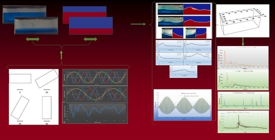
In this study, various experimental tests were performed on a rectangular tank with plan dimensions of 755 × 300 mm and height of 300 mm. A uni-axial shaking table was used to apply base excitations to the tank. To investigate the bidirectional effect of excitation, the tank was placed on the shaking table in four different orientations of 0°, 30°, 60°, 90°, as shown in Figure 2. The tank was made of plexiglass with a density of 1190 kg/m³ and a uniform thickness of 10 mm meaning that $\raisebox{1ex}{$t$}\!\left/ \!\raisebox{-1ex}{$b$}\right.=\raisebox{1ex}{$t$}\!\left/ \!\raisebox{-1ex}{$h$}\right.=\raisebox{1ex}{$1$}\!\left/ \!\raisebox{-1ex}{$30$}\right.$ and was fully fixed at the base. It is worth noting that plexiglass has an elastic modulus of 3.0 GPa. In addition, a blue color was added to ease the observation of the sloshing height. The experimental setup is shown in Figure 3. The tank was filled to 1/3 and 2/3 of its height with colored water for each orientation in order to observe the effect of orientation on changes in the liquid free surface and the associated pressure on the walls and roof of the tank. It should be noted that the tank wall flexibility has little effect on sloshing response, but it can affect the impulsive component with little effect on the convective part. It should be noted that the experimental study is used as a means for verification of the numerical model. The size of the tank in this study was chosen based on the available laboratory equipment, particularly the size of the shaking table, considering the length-width-height ratios of tanks commonly used in industry and that the tank’s orientation on the shaking table changes from 0° to 90°.

The tests were recorded from two directions by two high-speed HD video cameras. The cameras were placed perpendicular to the tank and were fixed to the floor. Following the tests, the videos were analyzed frame-by-frame to investigate the liquid surface for each test case.

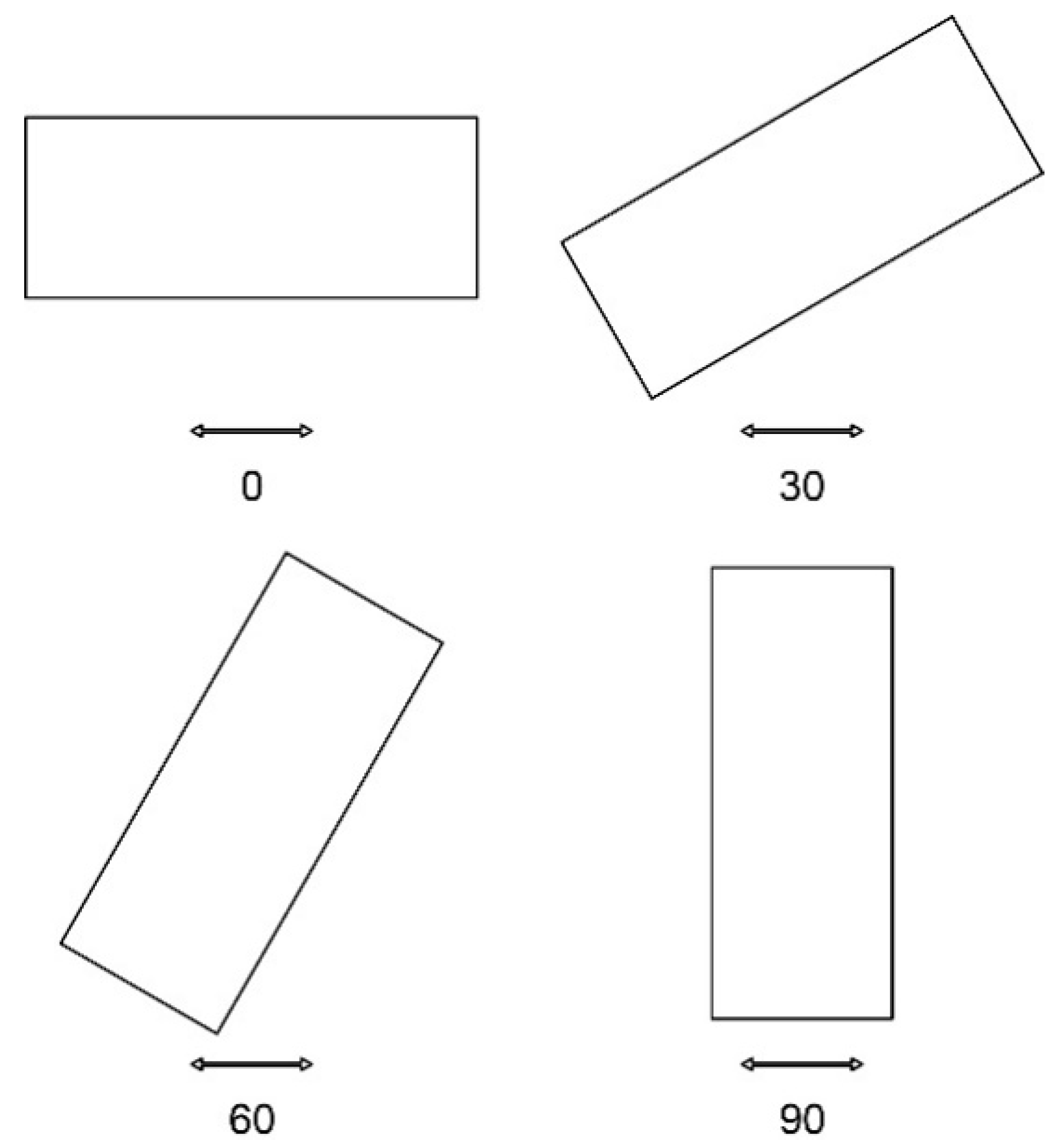
An earthquake excitation was applied to the tank. A study by Kianoush and Ghaemmaghami (2011) [45] compared the effect of four different earthquakes on a tank using the finite element method (FEM), and found that the longitudinal component of the 1940 El Centro earthquake caused the highest sloshing heights in the tank. Therefore, the N-S component of the 1940 El Centro ground motion was used in this study. The earthquake was used as recorded, i.e., with a scale equal to one. The acceleration, velocity, and displacement graphs of this earthquake with maximum values of 0.319 g, 361.4 mm/s (i.e., maximum absolute value), and (−213.4:+28.6) mm respectively are shown in Figure 4 [46].

Three harmonic sinusoidal base excitations with different frequencies were applied to the tank for a period of 60 s, which included the first convective frequencies of the tank and two other excitations within ±50% of that frequency. In order to apply the same excitation to the tank with different orientations, the frequencies were calculated based on the 0° orientation and applied to all cases investigated in this study. The total movement domain for the sinusoidal excitations was 70 mm (i.e., about 10% of the tank length), and hence the displacement amplitude was 35 mm (close to 5% of the length). The resonance frequency used was calculated based on formulations provided by Housner (1963) [6]. The displacement response histories for the 1/3 and 2/3 fill depths (i.e., 100 mm and 200 mm respectively) are presented in Figure 5a,b respectively.

A harmonic sinusoidal wave can be described by the following equation:

$$\mathrm{U}\left(\mathrm{t}\right)=\mathrm{A} \sin \mathsf{\omega }\mathrm{t}$$

(10)

where U is the displacement (mm), A is the displacement amplitude (mm), ω is the excitation frequency (rad/s), and t is the time (s).

The values chosen for ω in each case are presented in

Table 1. Applied frequencies for harmonic excitations.

Case	Frequency (rad/s)
100 mm liquid depth	Lower than resonance	2.02
	Resonance	4.03
	Higher than resonance	6.05
200 mm liquid depth	Lower than resonance	2.65
	Resonance	5.30
	Higher than resonance	7.95

.

Frames captured from the videotape of each experimental test were compared with the ones of the matching simulation from the numerical study in order to validate the numerical model. The results from the numerical model and experimental tests were compared for all the excitation types, frequencies, and orientations.

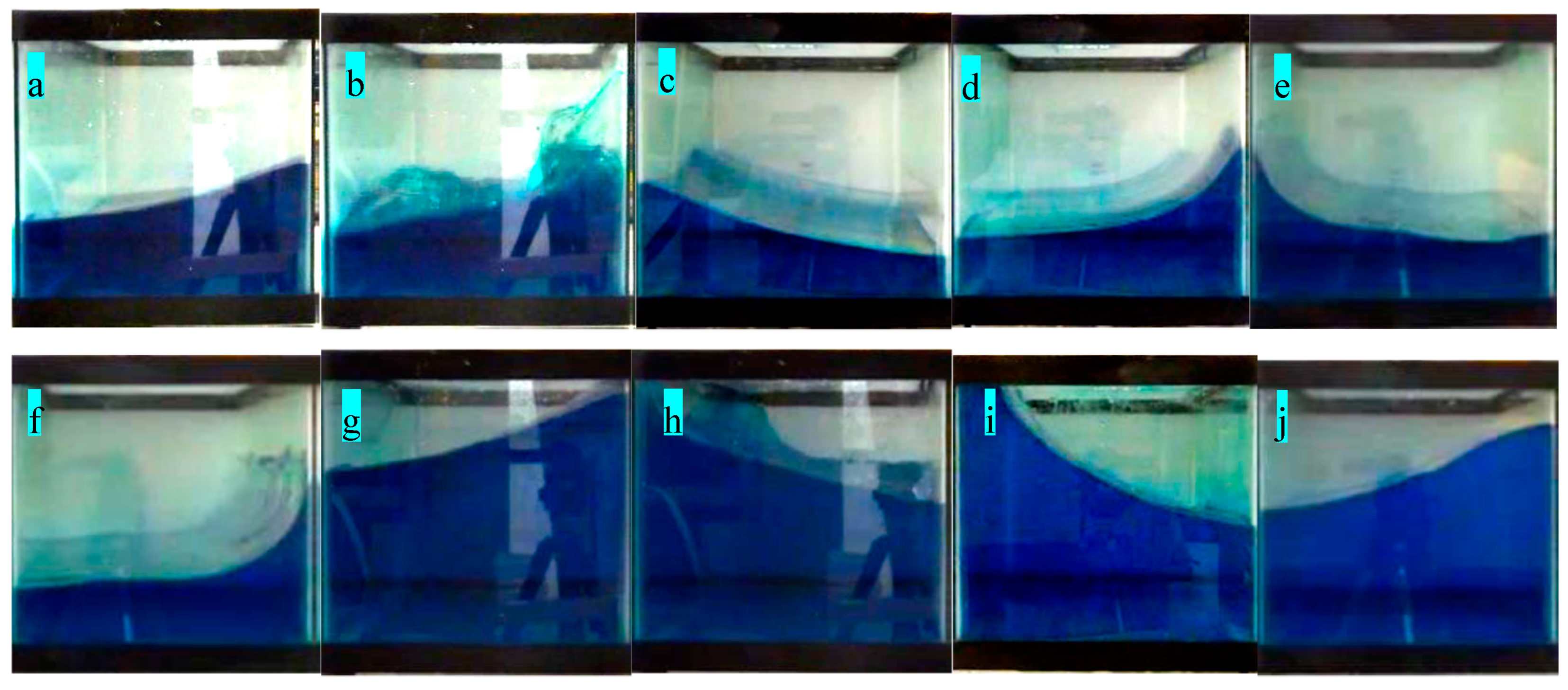
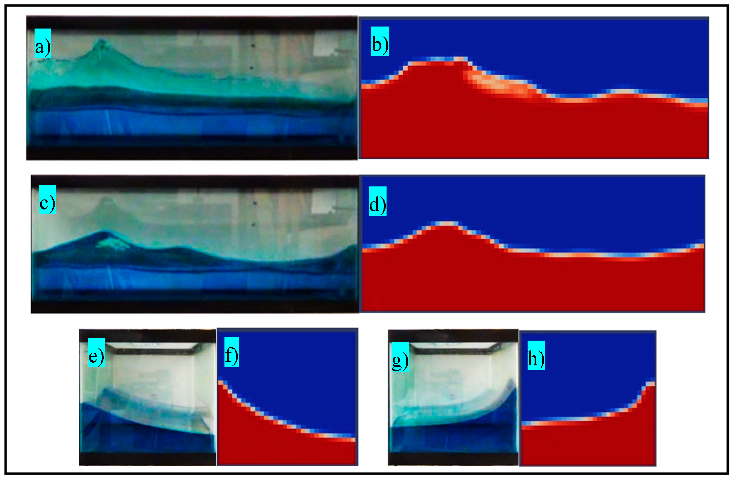
It was observed from the experimental tests that the sloshing height was amplified at the tank corners in comparison with other locations of the tank. This amplification occurred regardless of the tank orientation or the liquid height, and some cases are presented in Figure 6. These include: (a) 100 mm liquid depth, 0° orientation, lower than resonance frequency; (b) 100 mm liquid depth, 30° orientation, resonance frequency; (c) 100 mm liquid depth, 30° orientation, higher than resonance frequency; (d) 100 mm liquid depth, 60° orientation, higher than resonance frequency; (e) 100 mm liquid depth, 60° orientation, resonance frequency; (f) 100 mm liquid depth, 90° orientation, higher than resonance frequency; (g) 200 mm liquid depth, 0° orientation, higher than resonance frequency; (h) 200 mm liquid depth, 30° orientation, resonance frequency; (i) 200 mm liquid depth, 60° orientation, higher than resonance frequency; and (j) 200 mm liquid depth, 90° orientation, lower than resonance frequency. Higher sloshing heights at the corners can lead to higher pressures at those corners, including roof corners, compared to other locations. In a tank that is not aligned with the excitation direction (i.e., has a different orientation), the sloshing height at the corners is even higher than when the tank is aligned with the excitation.

2.4. Numerical Modelling

The OpenFOAM application was used for the numerical modeling of the tank. It is an open-source computational fluid dynamics (CFD) software capable of solving various problems from dam breaks to heat transfers. A large variety of CFD solvers are available in this application that can be used in the desired cases [47,48]. The adopted numerical method was the finite volume method (FVM). In this method, the time is divided into time-steps (e.g., 0.02 s) and the liquid volume is broken down into finite volumes. The Navier–Stokes equations are solved for each finite volume at each time-step. The results are then combined, and the answer to the equation is formed for the control volume. It should be noted that the Navier–Stokes equations are non-linear, and hence OpenFOAM uses non-linear methods to solve them.

A variety of turbulence models can be used with this software [23]. The OpenFOAM solver used in this study was interDyMFoam, which has the ability to solve problems with dynamic mesh. In this solver, the pressure correction algorithm PIMPLE (which develops a non-linear set of equations and solves them using an iterative approach) was used for the fluid flow and the volume of fluid (VOF) method was adopted for tracking the free surface. The PIMPLE algorithm is a combination of the PISO (pressure implicit with splitting of operator) and SIMPLE (semi-implicit method for pressure-linked equations) algorithms. While PISO and PIMPLE algorithms are applicable in transient cases, SIMPLE is used for steady-state problems. However, they are all iterative solvers.

The finite volume method adopted by OpenFOAM is based on a structured mesh with non-uniform distribution. The dynamic properties of each control volume are defined by its centroid. The mesh allows for an unlimited number of points per face per control volume. In the numerical analysis, the Van Leer method is used for divergence, a corrected Gauss linear scheme is used for Laplacian terms and a linear approach is used for interpolation. An adoptive time increment is used in this analysis, meaning that each time step is chosen based on the previous time step to increase the accuracy; however, the computational cost and time increases with this scheme. In terms of turbulence, a constant eddy viscosity model is chosen in this study, as it has less computational cost and does not affect the results.

The VOF method introduced by Hirt and Nichols (1981) [49] was used in conjunction with other numerical methods to track the free surface. In this method, a function F is defined with the value of one for every spot that fluid exists and zero for other points. In each cell, the average value of F shows how much of that cell is filled with fluid. Hence, the unit value of F means the cell is fully filled by fluid, and zero means there is no fluid in the cell. An F-value between zero and one shows there is a free surface in that cell. Thus, the free surface can be tracked.

In the current study, the first step was to validate the model by using the frames captured from the videos of the experimental tests and comparing them with the ones from the numerical simulations, as shown in Figure 7. In this figure, the images from the numerical model and the experimental tests do not demonstrate the same times, but they were captured from the same excitation phase. The reason for this time difference is that the shaking table takes a slightly longer time (approximately half a second) to start operating. In other words, the shaking table’s motion has a half-second lag from the input time-history. Following the validation, pressure sensors were placed at various locations on the roof of the tank in the numerical model, and simulations were conducted to find the maximum liquid pressure on the tank roof under both harmonic and earthquake excitation.

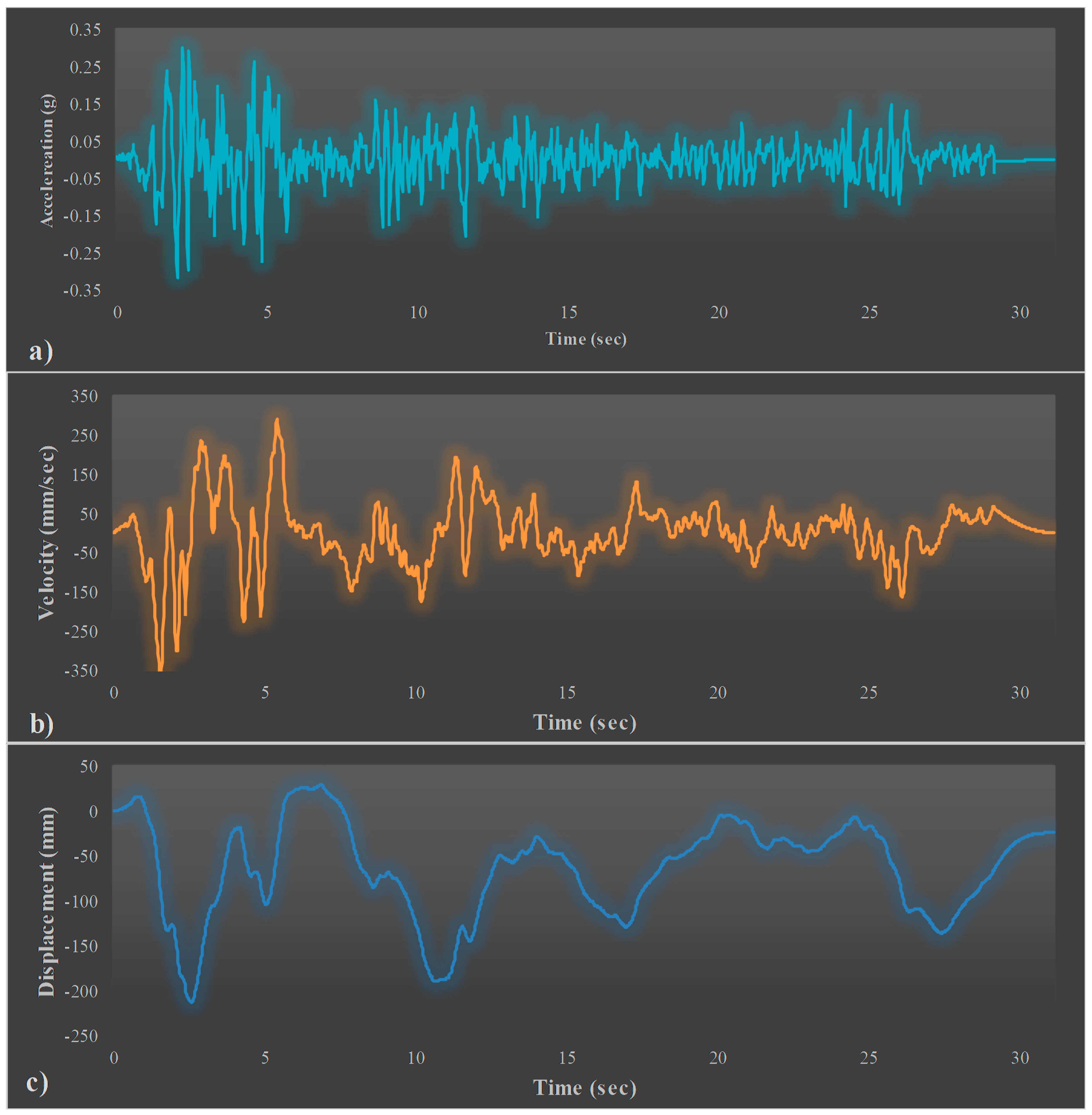
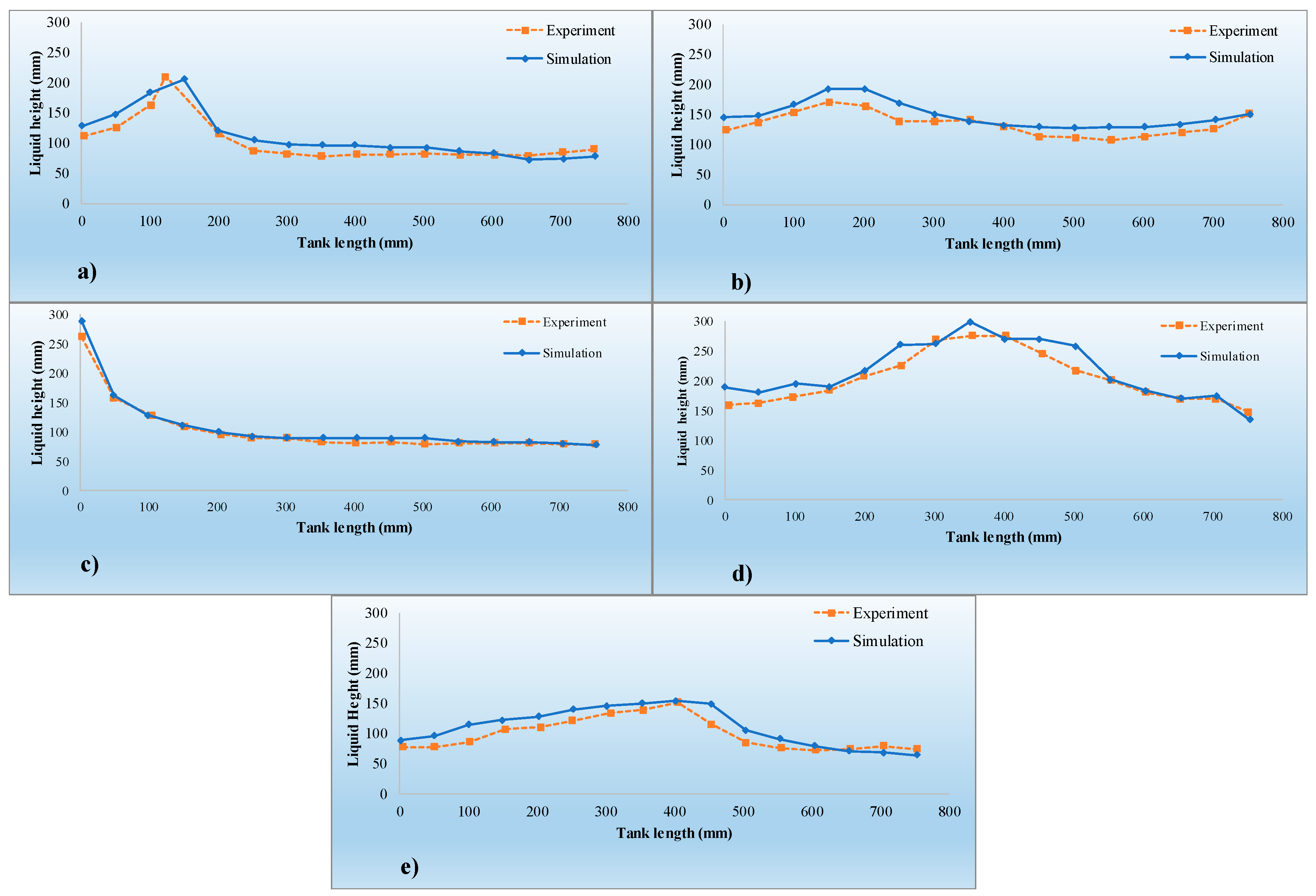
To validate the model, in addition to the qualitative comparison, the liquid surface was also digitized using MATLAB for a more detailed comparison in several cases. Figure 8 shows the free surface of the liquid considering five cases, and indicate the water height in the tank, free surface, and tank orientation. A typical time-step where a significant variation was observed was chosen for the presented cases in this figure. Then, the liquid height difference at the time step was calculated, squared, summed up, and divided by the total number of calculated points in order to find the root mean square error (RMSE) for the two sets of data. Finally, the RMSE value was calculated, as shown in Figure 8. The RMSE values ranged between 8.21 mm and 19 mm (i.e., error in the range of 1.09% to 2.53% of the tank length), which shows an acceptable agreement between the numerical model and the experimental results.

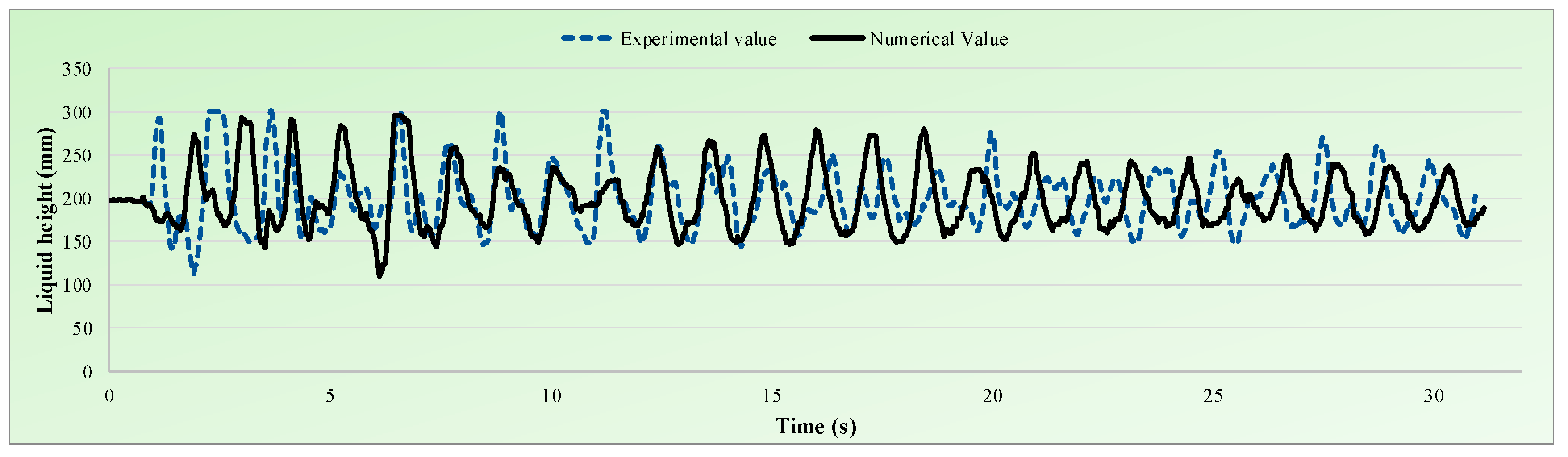
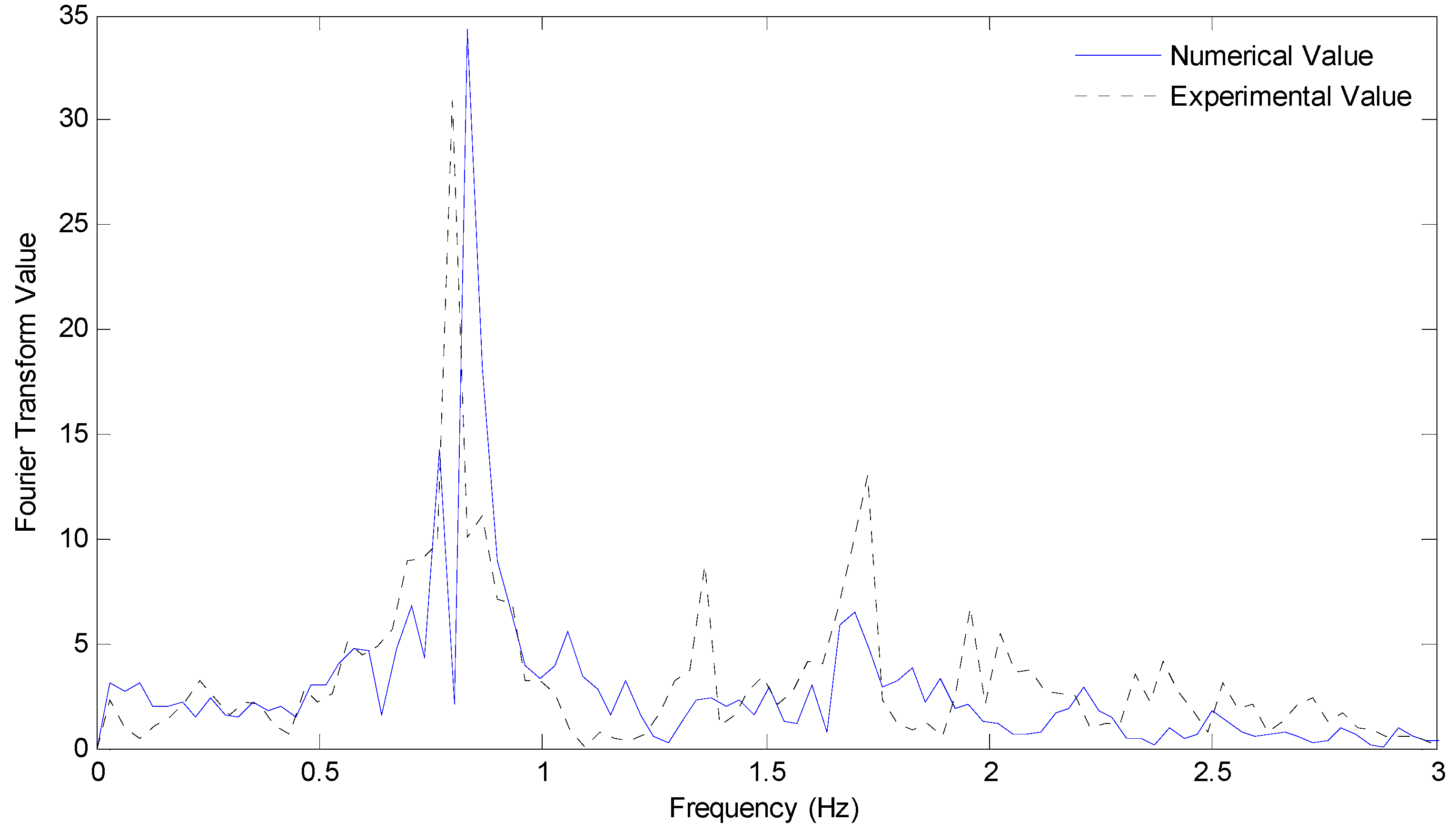
In addition to the liquid surface at different excitation phases, the liquid height over time at the corner of the tank was also measured in both numerical simulations and experimental tests for the earthquake excitations (Figure 9). The Fourier transform of the same parameter was compared for the two parts of the study (i.e., experimental tests and numerical simulations). Despite the complex dynamic behavior of the system, the maximum water elevation values are correctly predicted, but the differences increase over time due to the accumulation of errors. The comparison graphs (i.e., Figure 9) show that despite a delay at the beginning of the excitation (i.e., two seconds from the start time), the two graphs illustrate the same patterns and values for the rest of the time, especially for the time-span of 15 to 30 s where the liquid does not reach the tank roof. Additionally, a common way of comparing signals is to apply the Fourier transform to the two signals and compare them in Fourier space. It can be seen from Figure 10 that the Fourier transform in the numerical simulation’s spectrum is similar to the one from the experimental tests in terms of the dominant frequencies. In other words, the main frequencies obtained from the two graphs (0.797 Hz for the experimental study and 0.833 for the numerical study) only have a 4.5% difference.

Both the qualitative and quantitative comparisons between the numerical modeling and the experimental tests show that the performance of the model is reasonably accurate in predicting the motion of the liquid (whether the liquid motion is longitudinal or transverse) for all tank orientations and excitation frequencies. The model showed a good agreement with the tests concerning the liquid surface for the 0° and 90° orientations (i.e., uni-axial excitations), while some differences were observed for the 30° and 60° ones.

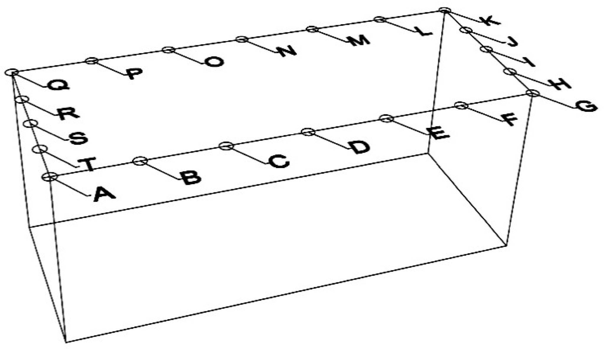
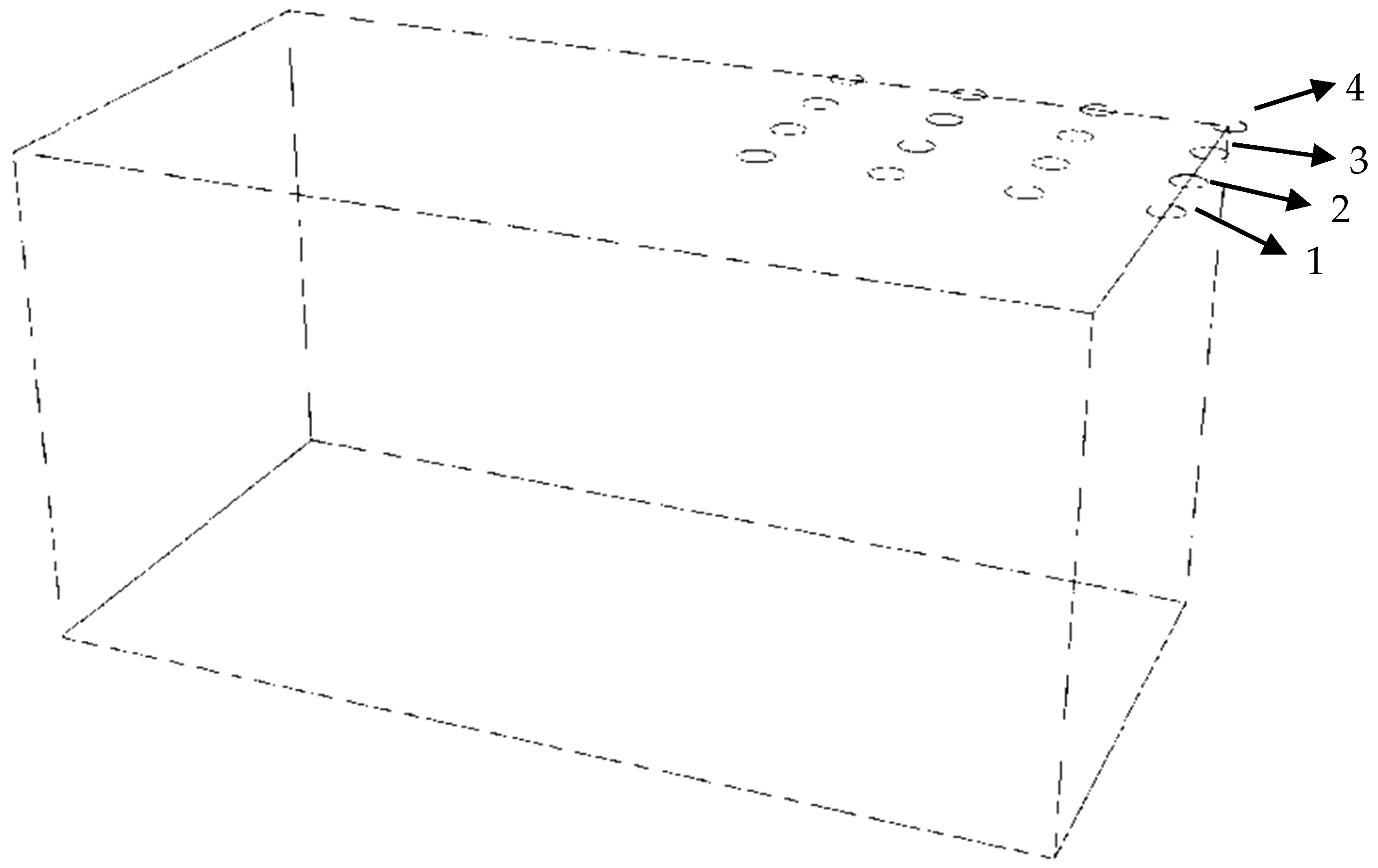
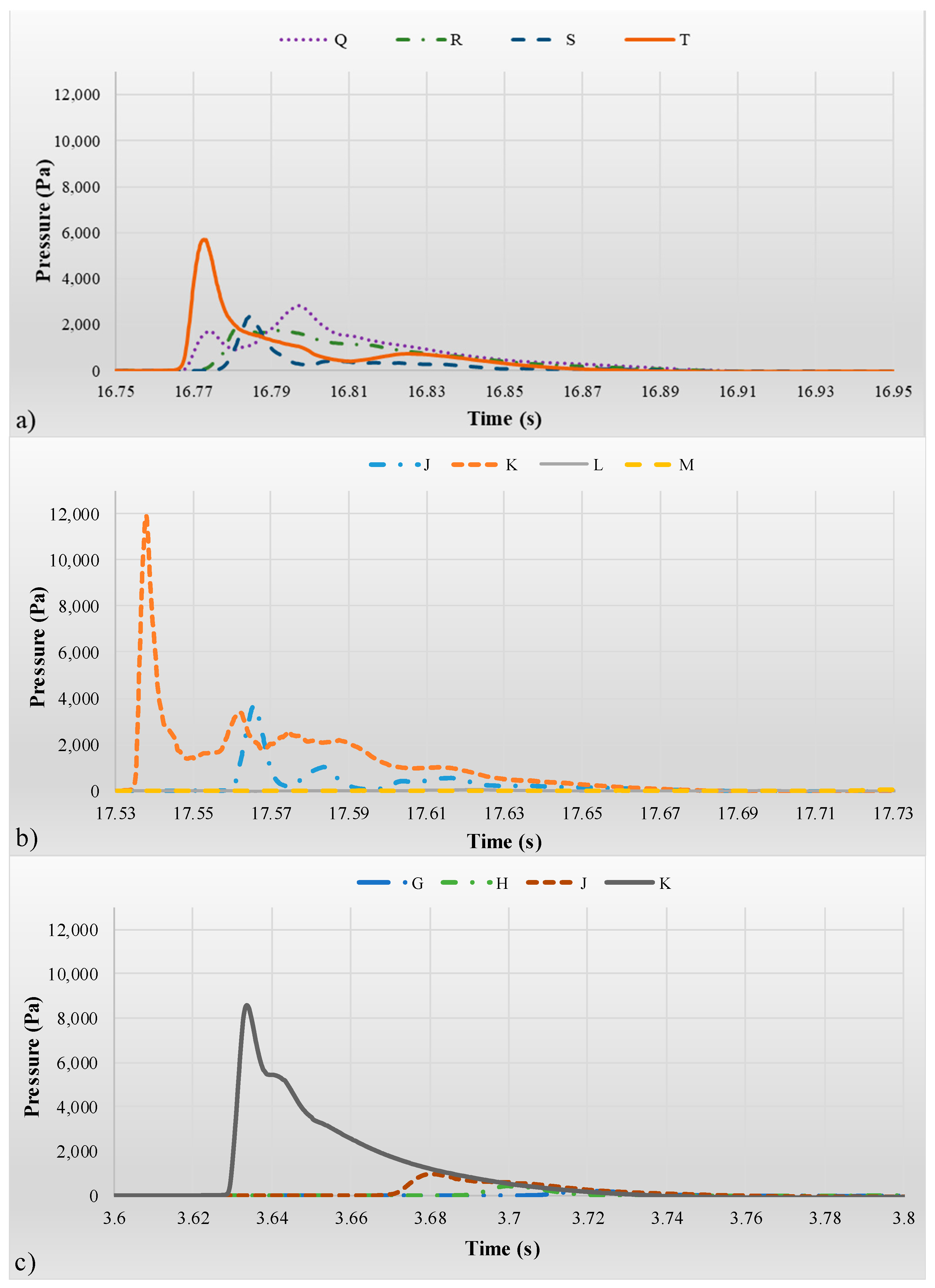
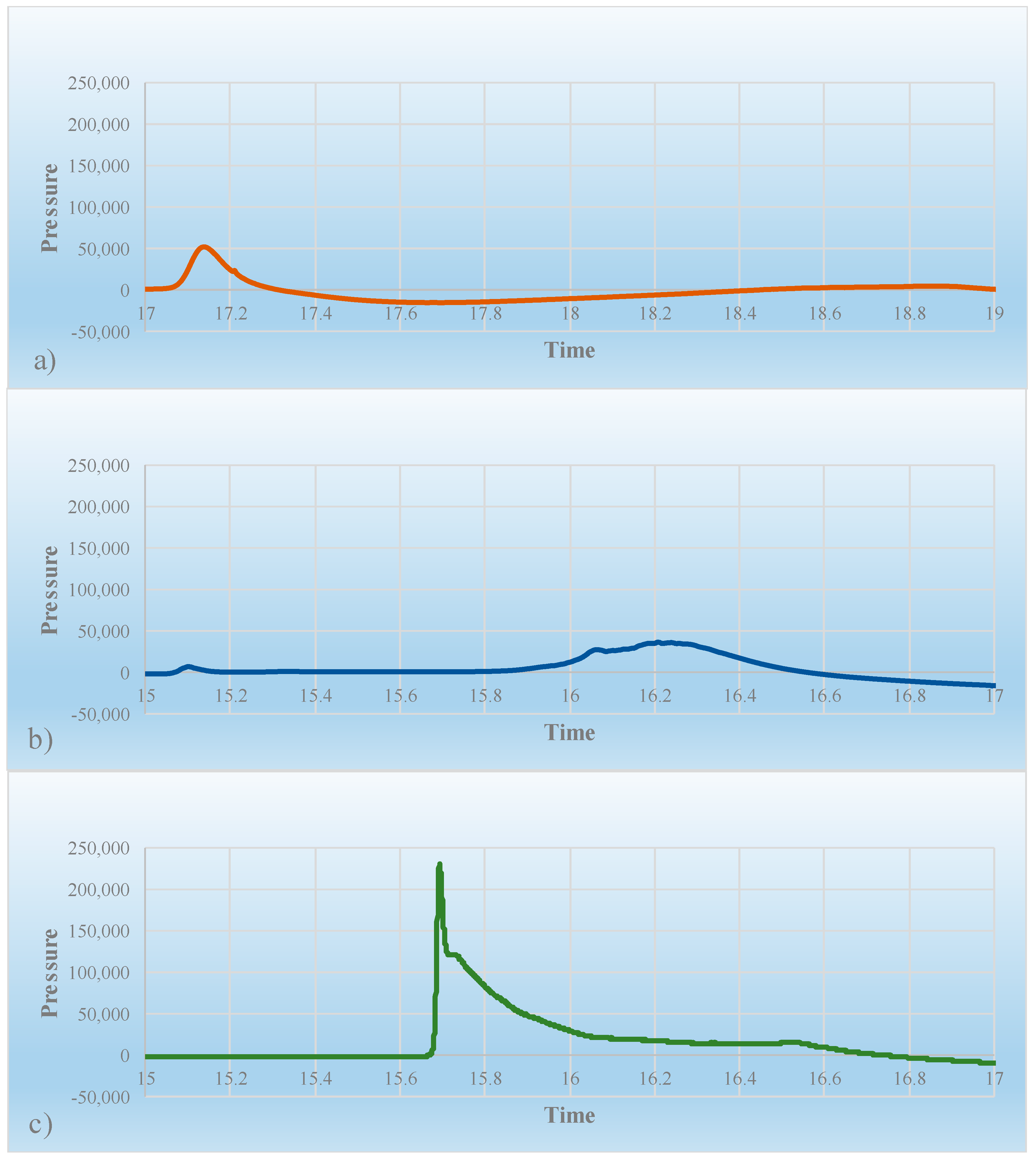
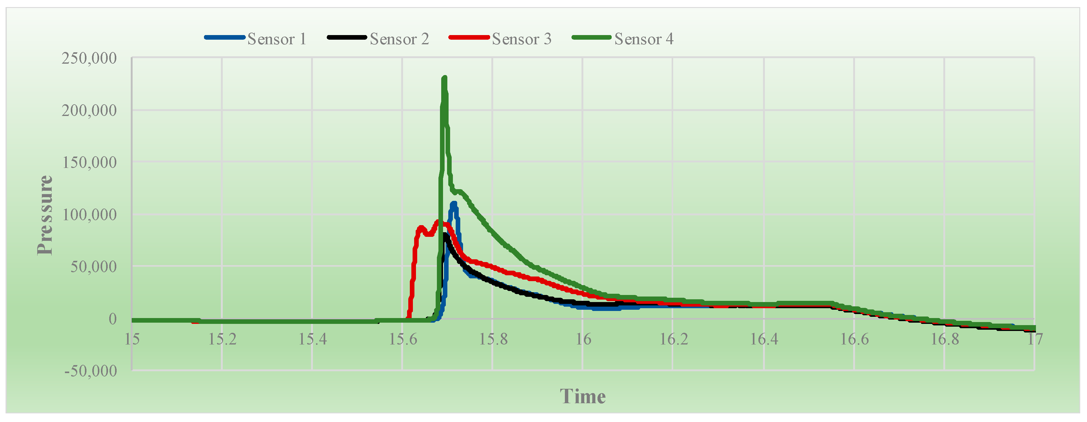
Once the numerical model was validated, pressure sensors were placed at various locations on the tank’s roof near the walls. Figure 11 shows the location of the sensors on the roof. Both earthquake and harmonic excitations were applied.

Following several trial and error cycles, it was found that the turbulent eddy viscosity of 2 ×10⁻⁴ m²/s led to the best results in terms of similarity of the free surface to the experimental work. After a reasonable calibration, the model was validated against the available experimental data. As mentioned earlier, an important goal in this study was to find a numerical model to predict the liquid surface behavior in a tank subjected to seismic loading, and hence the images from the experimental work and numerical simulations were compared to examine the validity of the proposed model. In this comparison, a number of cases were considered with respect to sloshing frequency, including frequencies higher than, equal to, and lower than the resonance frequency.

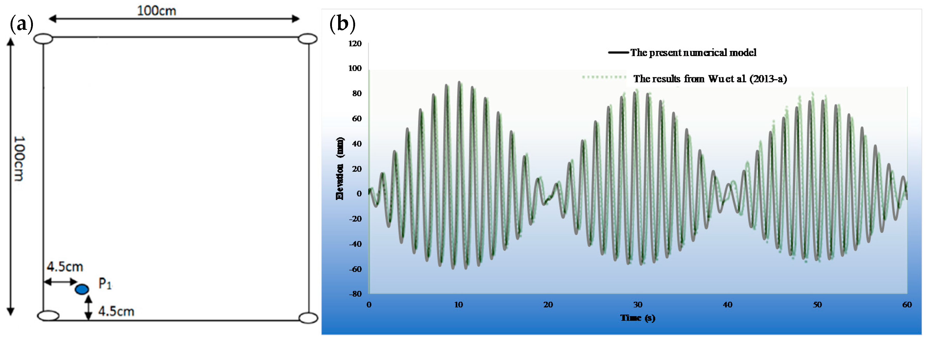
To further validate the model, the tank used by Wu et al. (2013-a) [38] was modeled in the OpenFOAM simulations for comparison. The water elevation was measured in the simulation and compared with the results from their study. The square-based tank with 1.0 m × 1.0 m plan dimensions and height of 1.0 m was partially filled with water up to a depth of 0.25 m, and a near-resonant frequency with an amplitude of 5 mm was applied. The results from the OpenFOAM simulations were compared with the experimental results from Wu et al. (2013-a) and are presented in Figure 12. A good agreement was found in terms of predicting the peak values; however, a slight shift in time is seen, possibly due to the locations of the probe in each study.

3. Results

Pressure Distribution

In this section, the results from the pressure sensors in the numerical study are presented and discussed.

From the simulations, the results from the pressure probes are presented in Figure 13 and Figure 14 for the tanks with 100 mm and 200 mm and different orientations, respectively. The figures show that regardless of the tank orientation and type of excitation, the tank’s corners show higher pressures irrespective of harmonic excitation (Figure 13) or earthquake excitation (Figure 14). In these figures, the time ranges that showed the highest variation were chosen. The pressure at the corners at times can reach up to three times higher than the pressure slightly away from the corners. An exception here is for the earthquake excitation applied on a 0°-oriented tank, in which the pressure on the tank’s wall does not show a significant difference between the corner and the middle of the wall.

Figure 15 shows the comparison of pressure for different orientations at sensor location K, located at the corner of the tank, under resonance excitation. It can be seen that when the orientation is changed from 0° to 30° or 60° (i.e., the excitation becomes bi-directional), the maximum pressures at the corners of the tank become higher compared to the ones from the uni-directional excitations (e.g., 0° orientation), and among the cases, the highest pressure was measured at the 30° orientation. It should be noted that in the 90° case, the water did not hit the roof; thus, the pressure for the 90° case was zero, and therefore not shown. The fact that an earthquake’s direction is not predictable requires attention for all these possibilities.

Based on the results from the numerical simulations, the excitation type has a significant effect on the calculated pressures in a sloshing tank. It was found that among the harmonic excitations, the resonance condition (i.e., when the tank is subject to the first convective mode frequency) creates the largest pressure values on the roof. The comparison between the harmonic resonance condition and the El Centro excitation also shows that the resonance condition is the worst case in terms of maximum pressure and can therefore be the most damaging. In Figure 16, the pressures caused by the resonance and earthquake excitations are compared, and shows that avoiding resonance conditions is ideal, although this is not always possible due to the randomness of earthquake motion.

In the next step, the maximum equivalent hydrostatic pressure in each case is calculated and compared with the hydrodynamic pressure values. In this case, a tank with the same plan dimensions but with taller walls was simulated. The reason for this was to explore whether a shallower tank can be replaced with a taller tank to determine if a measured equivalent hydrostatic pressure can be used as an estimation of the hydrodynamic pressure. This approach can lead to a simple calculation of hydrodynamic pressures in the absence of sensors. Furthermore, the computational cost of a hydrostatic numerical model will be significantly less expensive than a non-hydrostatic CFD model. The walls’ heights had sufficient freeboard for the liquid not to reach the tank roof. The same excitations as those for the tanks with short walls were applied, and the liquid height above the 300 mm level was measured (Figure 17). The height can be transformed into pressure as:

$$P_h=\rho .g.h_0$$

(11)

where ρ, g, and h₀ are the liquid density, gravitational acceleration and liquid height at a level above the top of the tank wall in the roofless tank (i.e., equal to the hydrostatic head that hits the roof in the tank with a roof) respectively.

Table 2. Maximum hydrodynamic pressure calculated at each sensor location and the equivalent hydrostatic pressure.

Liquid Depth (mm)	Excitation Type	Tank Orientation (Deg)	Maximum Pressure at Each Sensor Location (Pa)																				Maximum Hydrostatic Pressure at the Roof
			A **	B	C	D	E	F	G **	H	I	J	K **	L	M	N	O	P	Q **	R	S	T
200	Harmonic (resonance *)	0	6356	1241	310	1185	447	1372	9183	4587	4933	4672	6904	1264	727	129	377	1384	10,793	5787	6411	5652	8044
		30	8418	1779	262	368	210	1716	7940	7572	5375	3718	4779	753	480	454	916	758	8977	6676	6167	4546	8444
		60	2230	1831	744	334	137	1187	4119	3764	6438	6794	2163	991	174	158	225	1179	9144	6235	5148	3922	8357
	El Centro earthquake	0	641	2	5	33	111	842	2446	2430	2420	2431	2446	840	112	33	7	2	634	693	901	699	4616
		30	659	57	109	5	18	50	893	279	274	561	791	552	52	0	1	36	2665	1881	695	416	5132
		60	859	674	988	424	76	1179	1987	3	3	3	119	236	127	1	1	901	1801	1	0	0	4321
100	Harmonic (resonance *)	0	8641	1510	894	391	310	438	8822	4685	4175	6319	6700	1821	1049	666	278	1145	8187	8457	4988	7505	4068
		30	19,578	2633	474	929	1073	5144	9215	3768	5037	6306	12,333	1046	758	926	1407	4275	7142	6018	6067	6115	5172
		60	4082	2218	353	179	250	192	3378	1459	3413	5366	8573	4380	187	35	229	294	4618	2397	2487	2576	3337
	El Centro earthquake	0	1051	19	1	4	3	4	1028	1504	112	1099	270	4	3	3	71	18	1208	2067	2289	1798	530
		30	3111	639	295	366	1061	1157	1252	12	44	76	2780	602	63	9	16	1233	2451	373	438	502	2209
		60	658	641	623	397	1580	255	2433	246	221	196	1360	1085	811	891	1348	429	605	108	300	491	1344

* Resonance frequency is calculated based on a tank length of 755 mm. ** Sensor is located at the corner.

provides the maximum hydrodynamic pressures found at each sensor location for all harmonic resonance and El Centro earthquake excitations and also presents the calculated equivalent hydrostatic pressures for each excitation case for the tank with higher walls. In this table, columns A, G, K, Q represent the sensors located at the corners of the tank. It can be seen from the table that except for one case, the highest maximum hydrodynamic pressure occurs at the corners.

The table shows that in most cases, especially under harmonic excitation, the maximum hydrostatic pressure at the roof level is lower than the maximum hydrodynamic pressure, and the hydrodynamic pressure is up to four times higher than the equivalent hydrostatic pressure. There was one exception, i.e., when the tank with 200 mm water depth as compared to the 100 mm depth was excited by the El Centro earthquake, the hydrostatic pressure was higher than the hydrodynamic pressure. The increase in pressure ranged between 6% and 332%. The reason for this pressure variation could be due to the randomness of the earthquake motion.

The results of this part of the study demonstrate that the use of equivalent hydrostatic pressure will underestimate the dynamic pressure, and thus is not recommended.

4. Study on an Actual-Sized Tank

In this part of the study, an actual-sized tank with plan dimensions of 30 × 15 m and a height of 15 m is numerically simulated under base excitation with resonance frequencies. The goal here is to use the model that has been verified earlier in this study and compare the results of the model with the ACI350.3 (2006). The freeboard and the pressure at the roof of the tank are the parameters of interest. Sixteen sensors are placed on one quarter of the roof (Figure 18). These sensors can capture the pressure at the roof of the tank and locate where the maximum pressure could occur. The results are presented in Figure 19. These results demonstrate that even when sufficient freeboard is provided according to the ACI Code, which is the case for all three cases (see

Table 3. Comparison of available freeboard and the freeboard required by the ACI 350.3-06 and the maximum pressure at the roof with three different tank sizes.

Tank No.	Tank Height	Liquid Height	Available Free Board	Required Free Board Based on ACI	Maximum Pressure at the Roof
	mm	mm	mm	mm	kPa
1	300	100	200	116	19.6
		145	155	136	9.6
		200	100	153	8.9
		230	70	159	10.6
2	1200	700	500	269	29.3
		800	400	277	19.3
		900	300	283	25.4
		1000	200	287	16.4
3	15,000	10,000	5000	590	52.4
		12,000	3000	642	36.08
		14,000	1000	678	230.6

), the liquid pressure at the roof is significant. Also, two other tanks with total heights of 300 mm and 1200 mm are simulated, and the results are shown in the same table. In addition, the pressure-time history for sensors 1 to 4 is plotted for the 14-m liquid height in Figure 20. This figure shows a significant pressure surge at sensor number 4 compared to the rest of the sensors, which indicates that the corners of a tank’s roof need to be designed for much higher pressures when sufficient freeboard is not available.

5. Discussion

In this study, a rectangular liquid-containing tank of certain dimensions was tested both experimentally on a shaking table and numerically using the OpenFOAM software. The purpose of this study was to develop a numerical model to simulate the response of liquid storage tanks under seismic excitations. Various base excitations, including harmonic as well as a simulated historical earthquake, were applied to the base of a tank that was filled with water to 1/3 and 2/3 of its height. Various excitations were applied at four different horizontal orientations in order to consider the effects of bi-directional motion.

From both the experimental tests and the numerical modeling, good agreement was obtained with Housner’s simplified analytical model in predicting the frequency of the first convective mode of the liquid system. In other words, one can reasonably predict the frequency of the first mode of the liquid surface by using Housner’s simplified model. In addition, it was found that regardless of excitation type and frequency and the tank orientation on the shaking table, the sloshing height at the corners of the tank was higher than at other locations on the tank walls.

For the model validation, videotapes of the harmonic excitations were captured from the experiments, analyzed frame by frame, and compared to the frames from the same cycle of the numerical simulations. Since an earthquake in terms of frequency and amplitude is a random phenomenon, in order to validate the model for the applied simulated earthquake, in addition to the frame by frame comparison (i.e., same as the harmonic excitations), the response histories of the liquid height at one corner of the tank as well as the Fourier transform values of the liquid height were compared for the two parts of the study. Based on this evaluation, the validated model was used to estimate the pressures on the roof of the tank to determine the effect of such pressures at the corners of the tank in comparison with those at other locations on the roof.

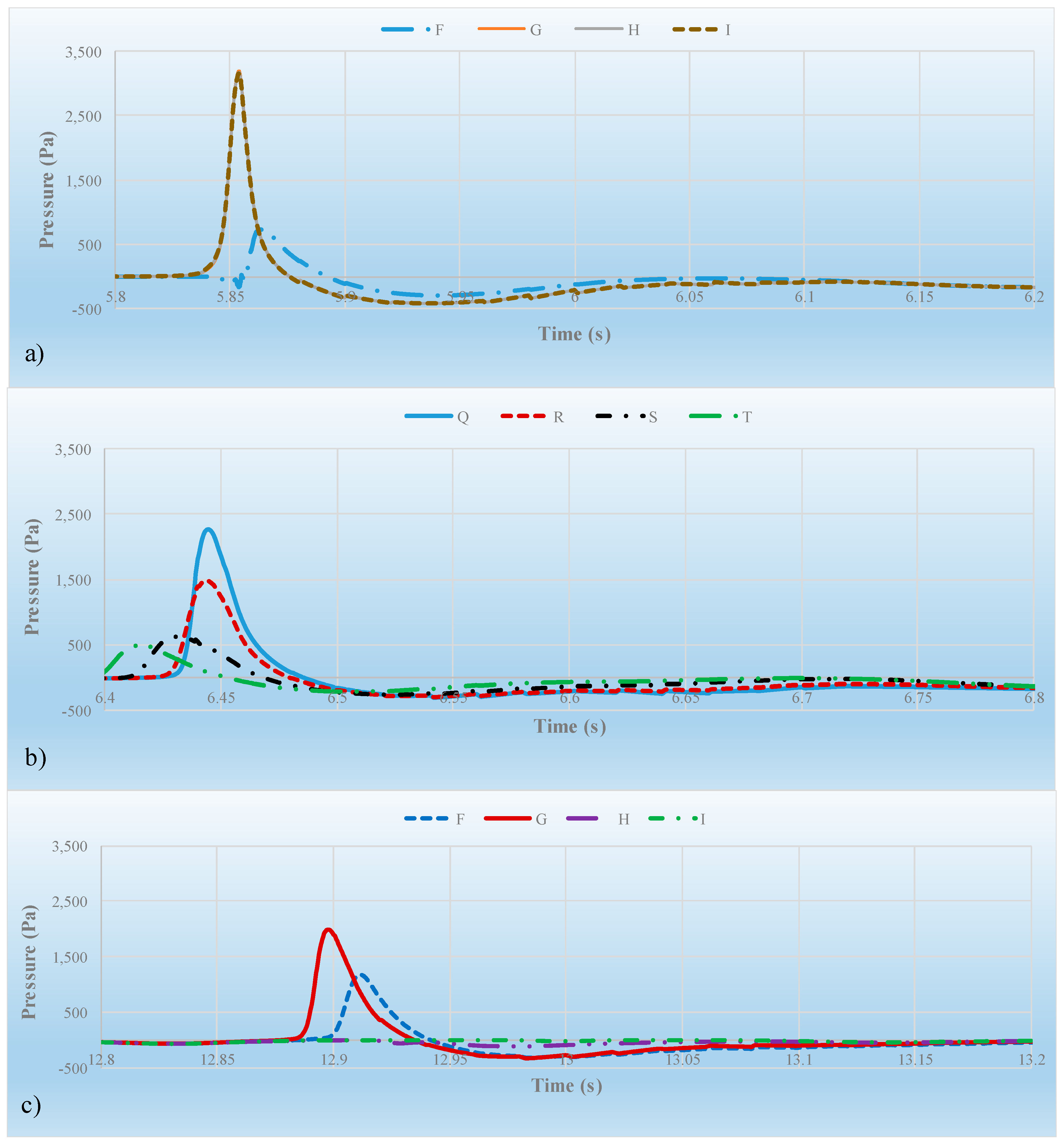
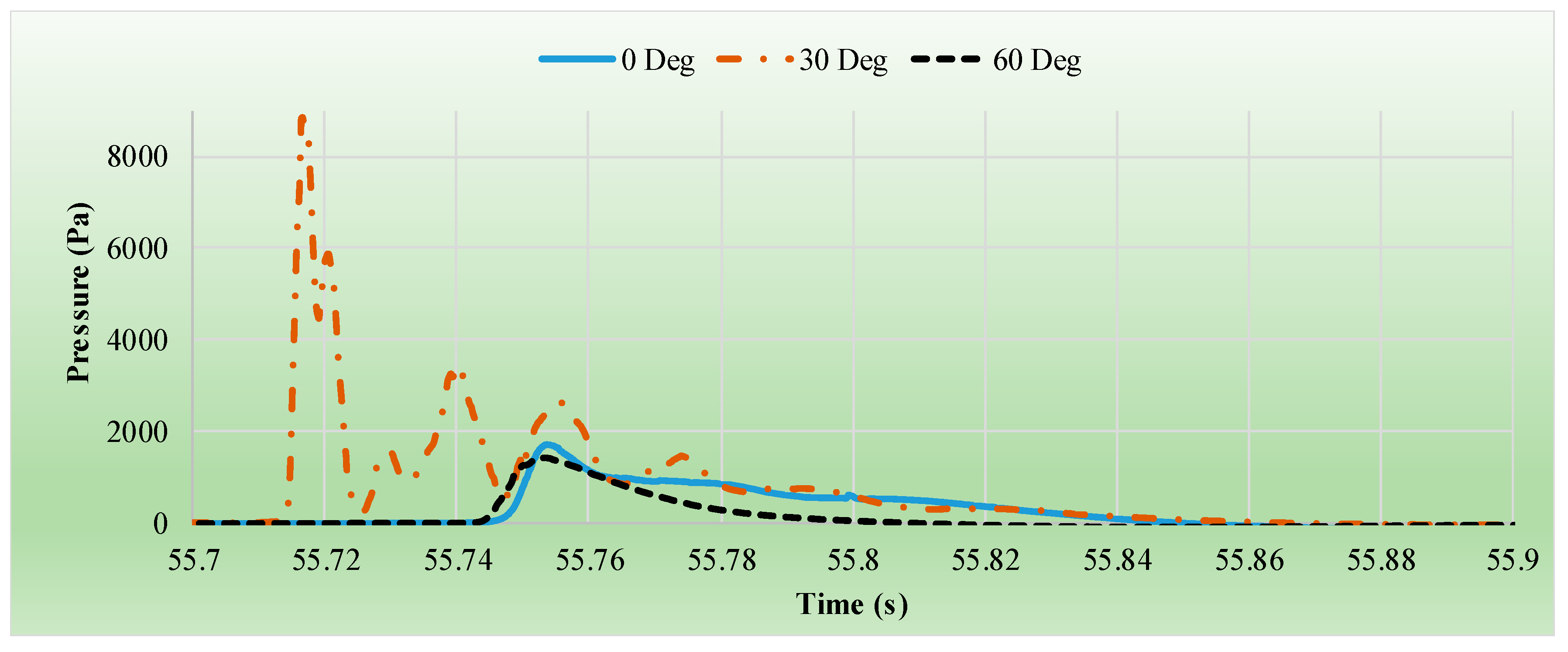
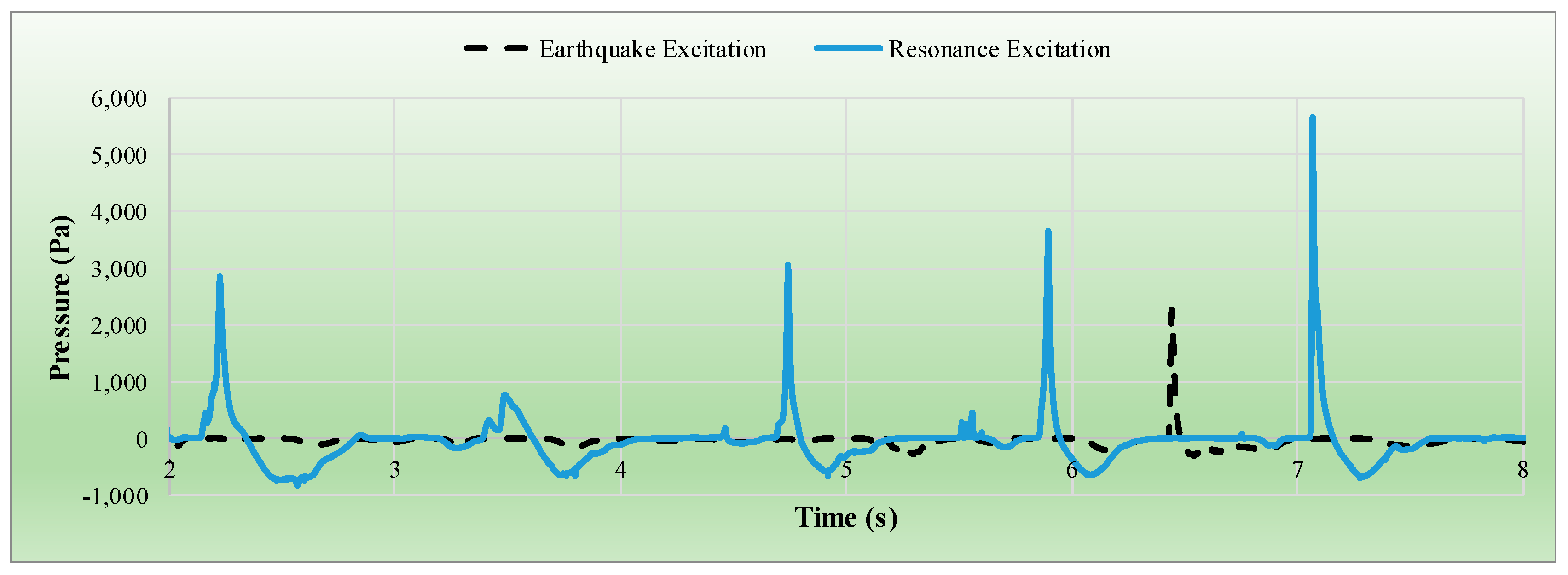
The data from the pressure sensors at the roof of the tank from the numerical simulations show that regardless of the excitation type and orientation of the tank, there was a higher maximum pressure at the corners of the tank in comparison with the other locations. In addition, for each excitation type, the maximum pressure at a corner of the tank excited in the 30- or 60-degree directions was higher than that of with single-directional excitations (i.e., 0° and 90° orientations). On this basis, it is recommended that design codes (e.g., ACI 350.3) consider higher pressure values at the corners of a tank when it may be subjected to ground motions. As such, the effect of bi-directional ground motion needs to be considered. Additionally, it is recommended to use a 3D CFD model to estimate such pressures.

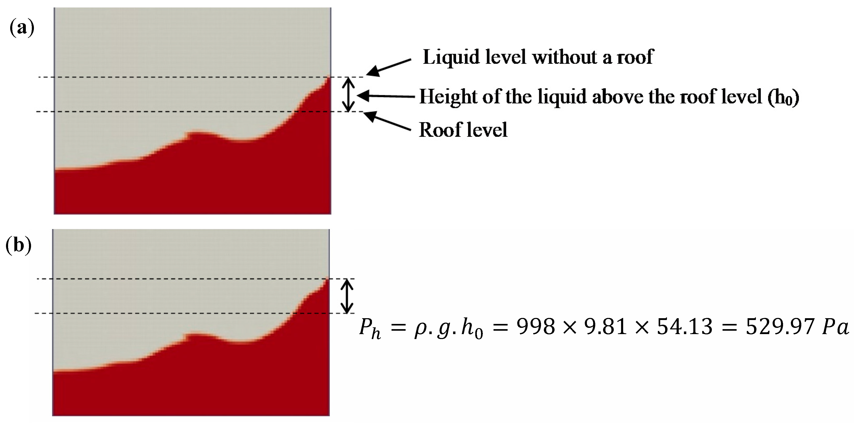
For the three tank sizes designed using ACI 350.3 code provisions and analyzed by providing the sufficient freeboard recommended by the code, it has been shown that the liquid height can exceed the wall height and cause impact pressure on the roof at the wall corners.