Landscape Planning of Infrastructure through Focus Points’ Clustering Analysis. Case Study: Plastiras Artificial Lake (Greece)

Abstract

Even though landscape quality is largely a subjective issue, the integration of infrastructure into landscapes has been identified as a key element of sustainability. In a spatial planning context, the landscape impacts that are generated by infrastructures are commonly quantified through visibility analysis. In this study, we develop a new method of visibility analysis and apply it in a case study of a reservoir (Plastiras dam in Greece). The methodology combines common visibility analysis with a stochastic tool for visual-impacts evaluation; points that generate high visual contrasts in landscapes are considered Focus Points (FPs) and their clustering in landscapes is analyzed trying to answer two questions: (1) How does the clustering of Focus Points (FPs) impact the aesthetic value of the landscape? (2) How can the visual impacts of these FPs be evaluated? Visual clustering is calculated utilizing a stochastic analysis of generated Zones of Theoretical Visibility. Based on the results, we argue that if the visual effect of groups of FPs is positive, then the optimal sitting of FPs should be in the direction of faint clustering, whereas if the effect is negative, the optimal sitting of FPs should be directed to intense clustering. In order to optimize the landscape integration of infrastructure, this method could be a useful analytical tool for environmental impact assessment or a monitoring tool for a project’s managing authorities. This is demonstrated through the case study of Plastiras’ reservoir, where the clustering of positively perceived FPs is found to be an overlooked attribute of its perception as a highly sustainable infrastructure project.

1. Introduction

The preservation of landscape as a part of natural and cultural heritage [1] is an important element for the sustainability of human development in a changing world [2]. The European Union defines the landscape as “an area, as perceived by people, whose character is the result of the action and interaction of natural and/or human factors” [3,4]. Changes to landscapes from infrastructure projects can be considered both positive [5], by the transformation of landscapes with respect to cultural and natural landscape elements, (b) and negative, by the transformation of landscapes with repeated use of industrial elements without landscape planning. In such cases, the development of infrastructure has been associated with the creation of political and economic problems due to the transformation of landscape [6,7].

The aesthetical value of the landscape is in its essence a political issue [3,8,9,10] that characterizes the socio-economic development and determines quality of life [11]. The aesthetic evaluation is widely accepted as a subjective process in philosophy [12]; thus, many researchers classify their approach as subjective [13,14,15,16,17]. On the other hand, other researchers have tried to find some objective rules, indicators, and proxies [18,19,20,21] to evaluate the aesthetical value of the landscape. Using modern technological tools such as Geographic Information System (GIS) analysis methods, decision makers are able to identify, for example, the most valuable or the most critical areas, according to their landscape value. Thus, such methods and their integration in policy help in the design both in short or medium-term and in the long-term [22,23,24]. Through image segmentation and other more sophisticated methods, researchers in the 21st century have tried to minimize the subjective elements of this issue and to quantify impacts with new indicators [25,26,27,28,29,30,31,32].

Schönthaler [33] notes that there must be a necessary reduction of complexity of environmental monitoring and a specific selection of a few and relevant variables in order to answer related questions. Following this rationale, in this paper, we define the clustering of Focus Points (FPs) as a simple method for the quantification of the impact of infrastructures on the aesthetic value of landscapes.

FPs are elements that attract our vision, which affect the perspective we have on a landscape. A FP is defined as the part of the landscape which is distinguished in terms of texture, color, or size and thus attracts vision [34]. A Magnetic Focus Point (MFP) is defined as the part of the landscape that has the characteristics of a FP and is also a pleasant aesthetic element [35].

We often see MFPs in our view. For example, an MFP can be a statue, a beautiful house, or a lake [36,37,38]. On the other hand, a common type of visually unpleasing or even repellent FPs are industrial installations or other civil infrastructures in landscapes.

It is widely accepted that the visibility of an FP impacts its environment. This so-called visual impact is in part subjective [39], and it can extend from a few centimeters if the examined FP is jewelry to several kilometers if the examined FP is a work of civil infrastructure (Figure 1). In terms of civil infrastructures, this visual impact of landscape is approached with methods of visibility analysis, e.g., with the mapping of Zones of Theoretical Visibility (ZTVs) [40,41,42,43].

In this study, we use a stochastic tool to develop a methodology for the quantitative evaluation of the results of visibility analyses. In particular, we utilize a stochastic tool (a) to investigate the transformation of original landscape views and (b) to evaluate the impact of clustering of FPs within a ZTV to the aesthetic value of the landscape. Then, we apply this methodology on an actual landscape transformed by a civil infrastructure project, i.e., a reservoir of a multipurpose dam, investigating how this methodology can be used for more sustainable landscape planning of civil infrastructure. We selected the case study of the artificial Plastiras Lake for this analysis, since we have collected extensive landscape-related public opinion data from previous research [47] that can now be re-examined with updated tools and allow for the comparison of results from past and current methodologies.

The mathematical field of Stochastics has been introduced on the opposite side of deterministic approaches as a way to model the so-called random, i.e., complex, unexplained or unpredictable, fluctuations observed in non-linear geophysical processes [48,49]. Stochastics helps develop a unified perception for natural phenomena and expel dichotomies such as random vs. deterministic. From the viewpoint of stochastics, there is no such thing as a “virus of randomness” that infects some phenomena to make them random, leaving other phenomena uninfected. Rather, both randomness and predictability coexist and are intrinsic to natural systems, which can be deterministic [50,51,52] and random at the same time, depending on the prediction horizon and the time scale [53]. This research aims to develop a stochastic analysis method to quantify both the spatial structures in terms of clustering as well as the temporal evolution thereof.

2. Methodology

A stochastic computational tool abbreviated 2D-C [54,55] is used to study the clustering in 2D space, using images from various sources. 2D-C measures the degree of variability (change in variability vs. scale) in images. Here, we refer to spatial scale, which is defined as the ratio of the area of k × k adjacent cells (i.e., scale k) that are averaged to form the (scaled) spatial field, over the spatial resolution of the original field (i.e., at scale 1).

Image processing typically begins with filtering or enhancing an image using techniques to extract more information from the images [56], and image segmentation is one of the basic problems in image analysis. The importance and utility of image segmentation has resulted in extensive research and numerous proposed approaches based on intensity, color, texture, etc., which are both automatic and interactive [57,58,59,60].

This analysis for image processing is based on a stochastic tool called climacogram. The term climacogram [61,62,63] comes from the Greek word “κλίμαξ”, which is pronounced: climax (meaning scale). It is defined as the (plot of) variance of the averaged process (assuming stationary) versus averaging scale k and is denoted as γ(k). The climacogram is useful for detecting both the short- and the long-term change (or else dependence, persistence, clustering) of a process, with the latter emerging particularly in complex systems as opposed to white-noise (absence of dependence) or Markov (i.e., short-range dependence) behavior [64].

In order to quantify the image variability, each image is first digitized in two dimensions (2D) based on a grayscale color intensity (thus, studying the brightness of an image), and the climacogram is calculated based on the geometric scales of adjacent pixels. Assuming that our sample is an area nΔ × nΔ, where n is the number of intervals (e.g., pixels) along each spatial direction and Δ is the discretization unit (determined by the image resolution, e.g., pixel length), the empirical classical estimator of the climacogram for a 2D process can be expressed as:

$$\underset{¯}{\widehat{\gamma }}\left(\kappa \right)=\frac{1}{n^2/{\kappa }^2-1}{\displaystyle \sum }_{i=1}^{n/\kappa }{\displaystyle \sum }_{j=1}^{n/\kappa }{\left({\underset{\_}{x}}_{i,j}^{\left(\kappa \right)}-\overline{\underset{\_}{x}}\right)}^2$$

(1)

where ${\underset{\_}{x}}_{i,j}^{\left(\kappa \right)}=\frac{1}{{\kappa }^2}{\displaystyle \sum }_{\psi =\kappa \left(j-1\right)+1}^{\kappa j}{\displaystyle \sum }_{\xi =\kappa \left(i-1\right)+1}^{\kappa i}{\underset{\_}{x}}_{\xi ,\psi }$ represents a local average of the space-averaged process at scale κ, and at grid cell (i, j), the ‘^’ over γ denotes estimate, and $\kappa$ is the the dimensionless spatial scale.

An important property of stochastic processes that characterizes the variability over scales is the Hurst–Kolmogorov (HK) behavior (persistence), which can be represented by the Hurst parameter [65]. This parameter is estimated by minimizing the fitting error between the empirical (observed) and the modeled (Equation (2)) climacogram, which are both derived from the large-scale values, i.e., the last 50 scales are used in the presented applications). The isotropic HK process with an arbitrary marginal distribution, i.e., the power-law decay of variance as a function of scale, is defined for a 1D or 2D process as:

$$\gamma \left(k\right)=\frac{\lambda }{{(k/\Delta )}^{2d\left(1-H\right)}}$$

(2)

where $\lambda$ is the variance at scale k = Δ, Δ is the time or space unit, d is the dimensionality of the process/field (i.e., for a 1D process d = 1, for a 2D field d = 2, etc.), and H is the Hurst parameter (0 < H < 1). For 0 < H < 0.5, the HK process exhibits an anti-persistent behavior, H = 0.5 corresponds to the white noise process, and for 0.5 < H < 1, the process exhibits persistence (i.e., clustering). In the case of clustering behavior due to the heterogeneity of the brightness of the image, the high variability in brightness persists, even in large scales. This clustering effect may substantially increase the diversity between the brightness in each pixel of the image, which is a phenomenon that is also observed in hydrometeorological processes (such as temperature, precipitation, wind etc. [49]), natural landscapes, and music [65].

The algorithm that generates the climacogram in 2D was developed in MATLAB for rectangular images [66]. In particular, for the current analysis, the images are cropped to 400 × 400 pixels, 14.11 cm × 14.11 cm, in 72 dpi (dots per inch).

This method has been introduced in the evaluation of the aesthetic of art paintings and landscape [54,55], so in order to exam the impact of clustering of MFP, we will see the following example.

3. Analysis

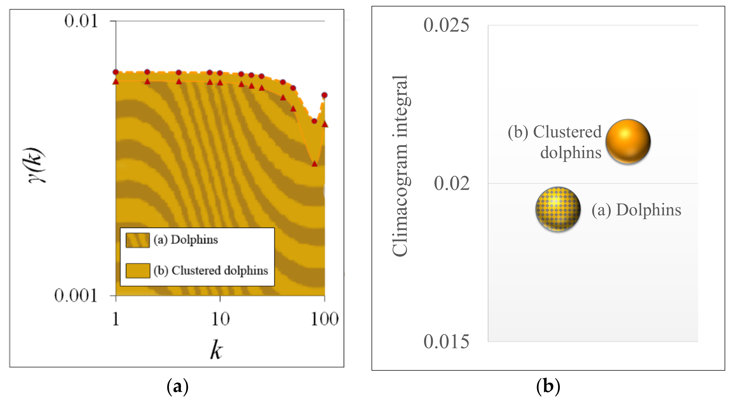
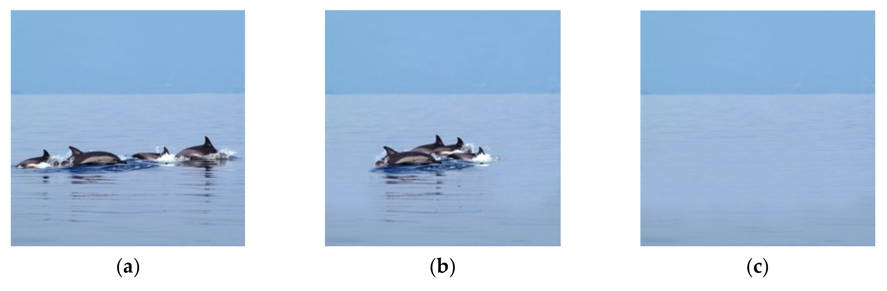
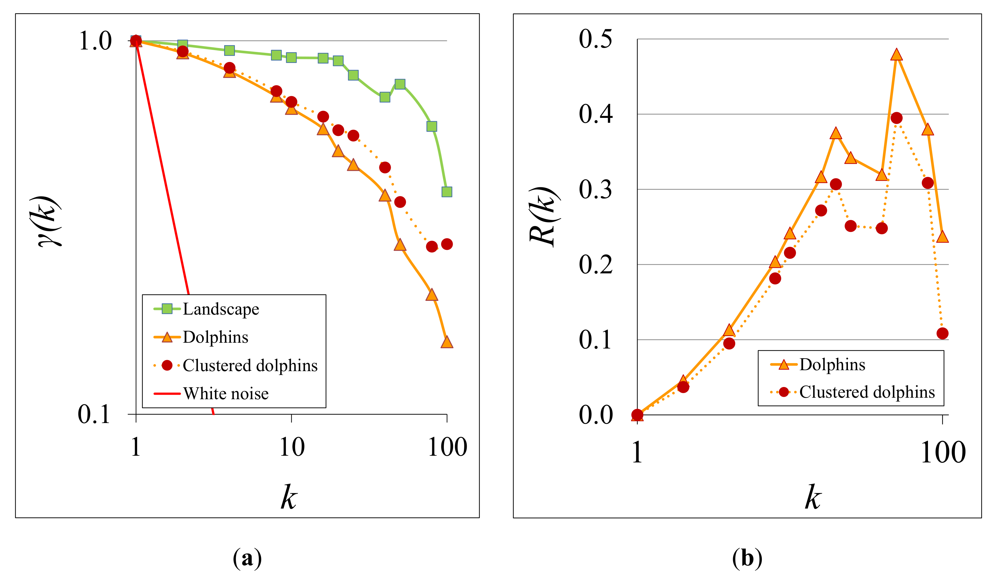
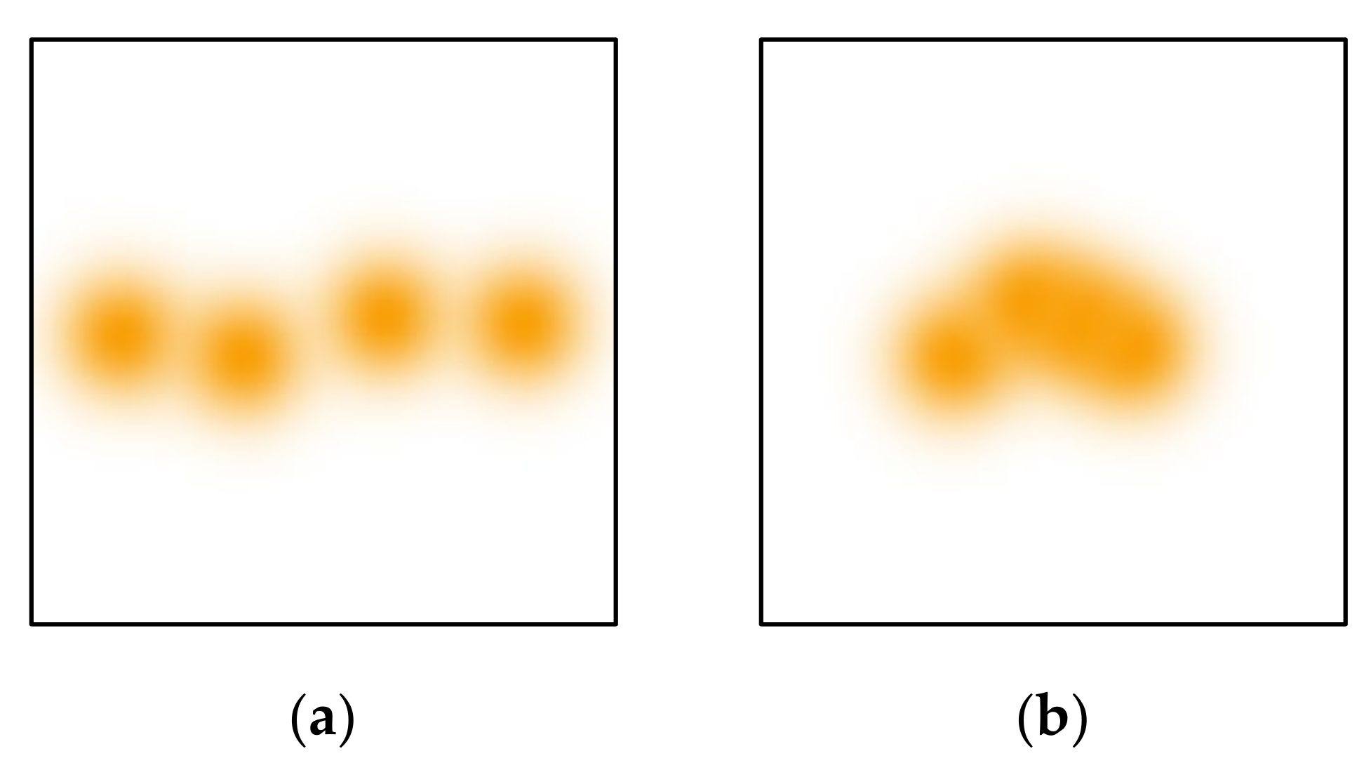
3.1. Clustering in the Analysis of Views of Objects

A FP can be perceived in different ways. One observer can view the FP without any barrier or filter in one part of the scenery, or through barriers or filters [67]. If an observer beholds an FP without any barrier or filter, then the FP is revealed intensively.

When an FP appears in the scenery, we have to examine how this FP can be discernible from different locations. This depends on the distance, the barriers, and the filters located between the FP and the observer.

A stochastic method is used to evaluate the transformation of an original image in a theoretical scenario of a sudden appearance of a herd of dolphins, which are obviously MFP. Different clustering arrangements of the herd are examined (Figure 2a,b), aiming to quantify the visual transformation to the examined scenery, using the original image that does not have any transformation as a baseline (Figure 2c).

A stochastic method has been developed for quantifying the transformation of the images based on 2D climacograms [54,55]. For the quantification of the difference between climacograms, we subtracted their values for each scale:

R(k) = γ(k) _{original image} − γ(k) _{transformed image}

(3)

where ${\gamma }_{\left(k\right)}$ are the climacogram estimations of the original image and the transformed image, respectively.

The results (Figure 3) indicate that the minimum alternation to the structure of the original image was caused when the herd of the dolphins was clustered.

3.2. Clustering in the Analysis of ZTV Sketches

Each FP has a ZTV, which is dependent on the size of the object and the terrain that surrounds it, as ZTV is calculated through a circular line-of-sight test around the examined object. The ZTV quantifies spatially the ability of the object to attract vision and thus the extents of its visual effects the environment. In Figure 3, we saw an example of clustered MFPs, which have smaller impact in the scenery than declustered MFPs.

Figure 4 presents the ZTVs of dolphins in Figure 2, which are characterized as (a) ZTVs with faint clustering and (b) ZTVs with intense clustering. The pixels analyzed are represented by numbers denoting their color intensity in grayscale (white = 1, black = 0). Previous related work shows the steps of this analysis in detail [68].

For the integration of all information contained in the 2D climacogram of each image, we evaluate the cumulative areas underneath each one for all scales (Figure 5a), i.e., the climacogram integral ${{\displaystyle \int }}_{\Delta }^k\gamma \left(x\right)/x\mathrm{d}x$, where Δ and k are the minimum and maximum scale, and we have divided by x in order for the integral to converge for arbitrarily high k ($k\to \infty$). In the discrete case, this can be approximated as:

$$\mathrm{CI}\left(k\right)={\displaystyle \sum }_{i=1}^{n\left(k\right)-1}\left(\gamma \left(x_{i+1}\right)+\gamma \left(x_i\right)\right) \frac{x_{i+1}-x_i}{x_{i+1}+x_i}$$

(4)

where i is the number of integration intervals up to scale k, x_j is the j_th scale, and n(k) is the number of scales up to k. We evaluate $\mathrm{CI}\left(k\right)$ at the maximum available spatial scale, so that it be the best approximation of the limit $\mathrm{CI}\left(\infty \right)$.

Figure 5b shows the results of the evaluation of clustering the herd of dolphins. High values of the climacogram integral show intense clustering, while small values show faint clustering, which is preferred when we have MFP.

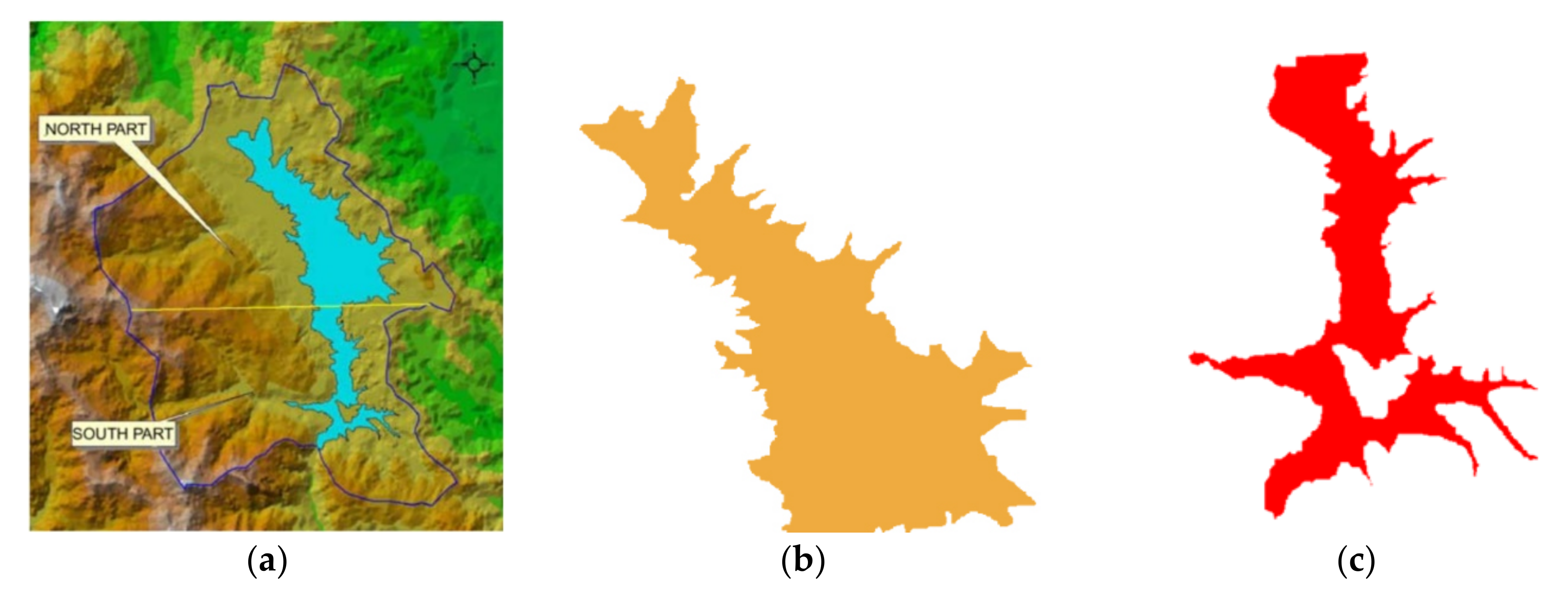
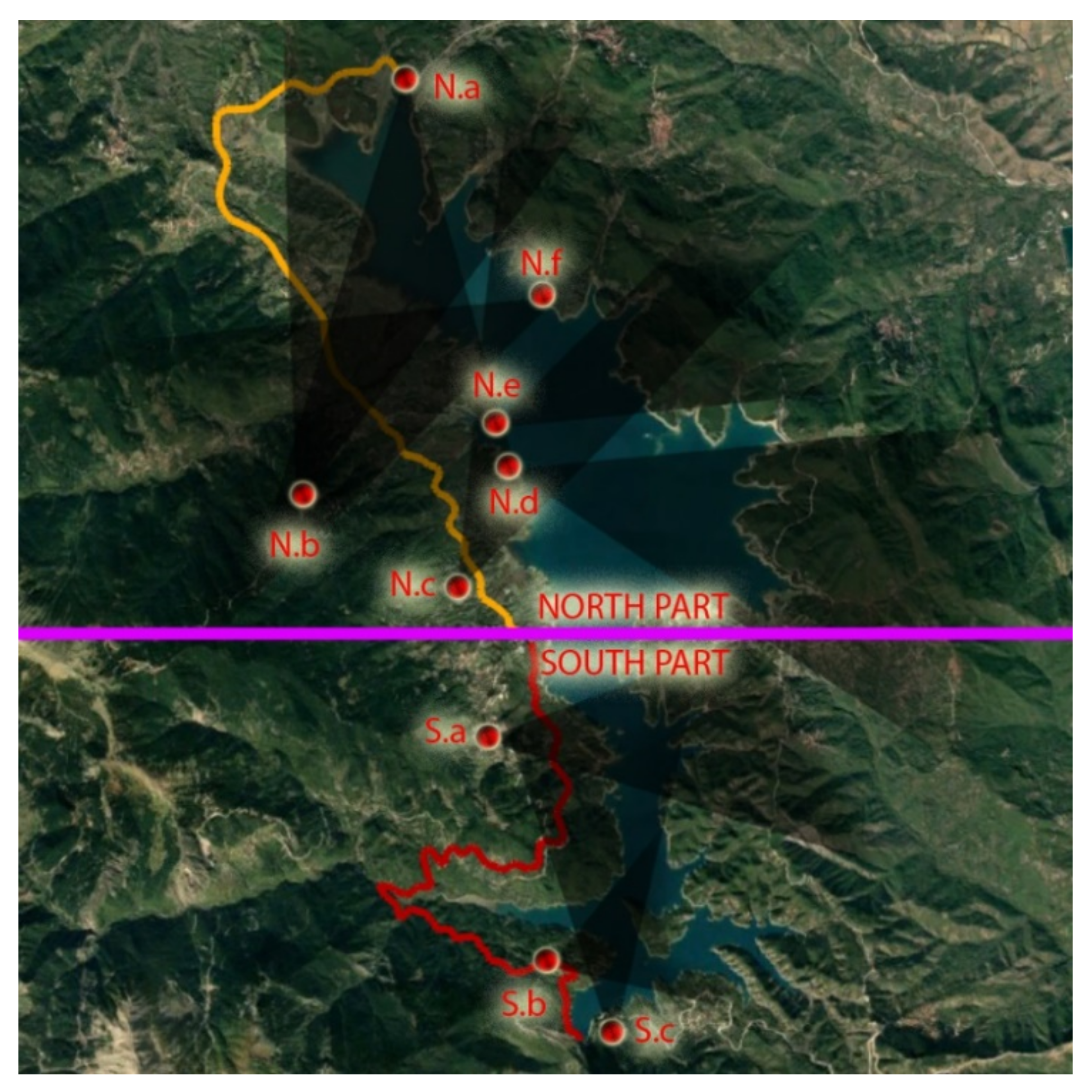
4. Case Study: Plastiras Lake

Plastiras reservoir is an artificial lake in Greece generated by the homonymous arched dam and famous for its beautiful landscape [69,70,71,72,73,74]. Plastiras Lake is a unique example of how civil infrastructures can be sustainably integrated into the landscape and create beautiful artificial landscapes that attract visitors and support a multi-dynamic sustainable development [69].

We chose this case study because previous work based on questionnaires (human judgment), theoretical analysis, and field research (Figure 6) of landscapes have shown that water is perceived as an MFP in the landscape and also that observers perceive the south part of the Plastiras reservoir (Figure 7, first row) as more beautiful than the north part of the reservoir (Figure 8 and Figure 9 first row) [70,71,72]. When an expert looks at data and images, this conclusion could be also reached due to other landscape-parameters, but in this case the validation of the positive character of the landscape by public perception is correlated with quantitative visibility analysis. Based on previous research, we can validate the presented-novel methodology utilizing the past knowledge of the problem and the public’s perception. Twenty years ago, when the initial analysis of the problem was carried out, we only had qualitative tools at our disposal.

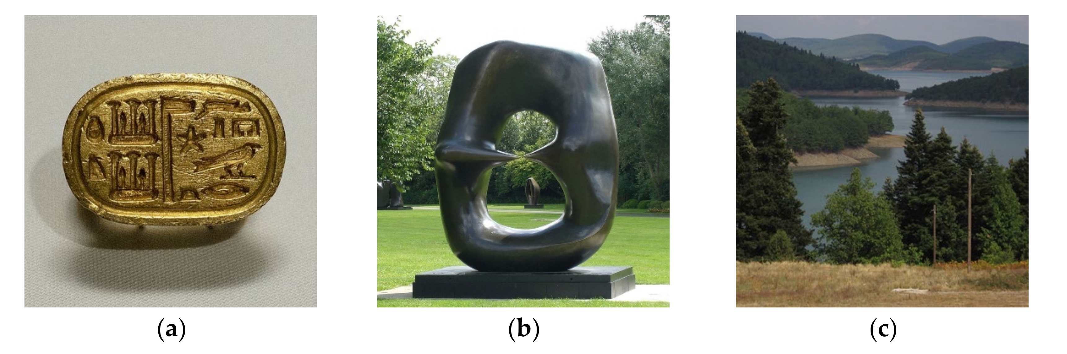
4.1. Clustering in the Analyis of Typical Views of the Reservoir

In order to evaluate the view of the landscape, we selected characteristic pictures from the database of our 2002 landscape research project [73]. Each picture is marked in the map (Figure 6), and the date of capture as well as the reservoir level have also been recorded. Obviously, an actual observer would be able to see an infinity of views as “pictures”. To summarize the authentic visual experience, we presented the most characteristic pictures, as extracted from the results of previous research that analyzed the aesthetics of the north and south part of the lake.

It is important to note that these pictures were selected because they are found in typical belvedere areas from where the landscape is most often viewed; the road does not offer neither a continuous view of the lake nor an abundance of spots for cars to stop or pedestrians to walk. Thus, the selected pictures express typical views (extracted from questionnaires) for the majority of the observers, meanwhile covering a significant area of the examined landscape.

Trying to quantify why the landscape of the south part is visually more pleasing than the landscape of the north part, we transformed photographs of the scenery (removing the lake), as can be seen in the second row of Figure 7, Figure 8 and Figure 9. The evaluation of the climacograms of the alteration of original images (including the lake) vs. transformed images (without the lake) of the landscape shows that the south part of the lake is transformed more intensively from the lake (Figure 10). This could explain why the observers are more impressed by the south part of the landscape and find its landscape more beautiful, as this part is more impacted by the landscape transformation in relation to the (theoretical) original image (without the lake), and obviously the impact is perceived as positive.

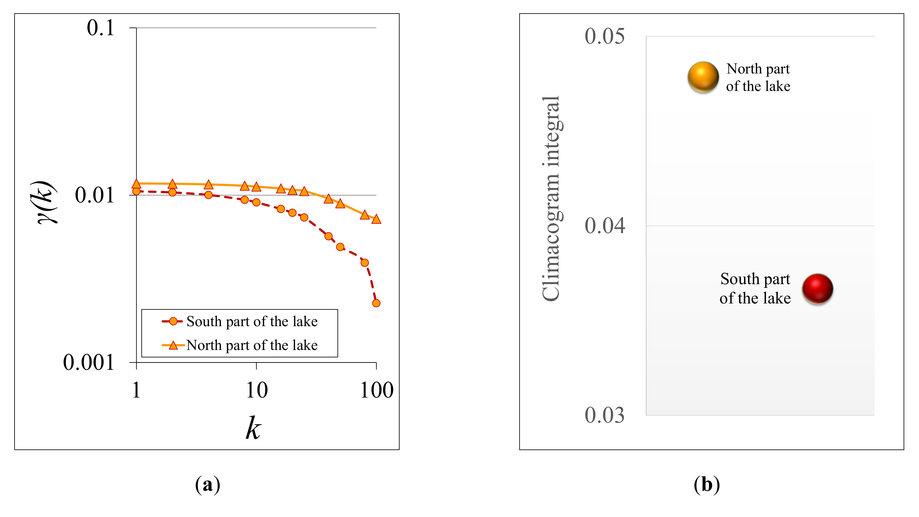
4.2. Clustering in the Analysis of ZTV Map

In order to evaluate the differences in the landscape integration of the reservoir in each case, due to the differentiation of water presence in the north and the south part of the lake (Figure 11), we evaluated the corresponding ZTV maps of the reservoir (Figure 12).

Investigating the clustering of the ZTVs, we calculated the ZTVs that correspond to the same road distance (≈ 11.5 km) for the north and south part of the landscape (Figure 13). As demonstrated in Figure 14, the results show that the south part of the lake has a fainter clustering of ZTV than the north part of the lake.

Faint clustering of ZTV in the south part of the landscape means that the lake, which is perceived as an MFP with positive landscape impact, has more spread dispersed visibility in the south part of the landscape than in the north part (Figure 14).

Therefore, minimum clustering and increased spread of an MFP in a landscape is positive to the observer, which is also intuitive and in accordance with previous research [58,59,60]. On the contrary, maximum clustering and limited spread of a negatively perceived FP can contribute to minimizing its landscape impact.

5. Discussion

Kant noted that “no objective rules of taste can be given which would determine what is beautiful through concepts” [8]. According to this note, evaluating the landscape with the tools at our disposal in the first stage of the research on the aesthetics of the landscape of Plastiras reservoir (during years 2000–2005) in the paper “Resolving conflicting objectives in the management of the Plastiras Lake: can we quantify beauty?” [74], we noted that: “This classification, [(of scenery)] especially in the level of detail in which it is presented, is only an indication, and is, to some extent, arbitrary; aesthetic quality is neither measurable nor objective, and there are no clear division lines”. Similar questions have also arisen in other articles [75]. On the contrary, Leibniz believed that there is a norm behind every aesthetic feeling, which we simply do not know how to measure [76].

It has to be noted though that a limitation of this study lies in the subjectivity related to which types of civil infrastructures are considered of negative impact to landscape and which are considered of positive effect. However, we believe that this limitation can be overcome by sight-specific [69,70,71,72] or specialized literature [37] that can limit, to an extent, the associated subjectivity through the statistical analysis of public perception; e.g. like in utilization of our past study of Plastiras reservoir in this study. On these terms, we could state that this study leans on the side of Leibniz’s philosophy on the existence of aesthetical norms as it proposes a quantitative tool for the sustainable landscape integration of infrastructures.

6. Conclusions

Works of technological and civil infrastructure support the needs of human society but also generate intense transformations to urban and natural landscapes at multiple scales and are perceived as FPs in landscapes [36]. These transformations become even more perceivable when they alter landscapes, urban or natural, of historical and cultural significance. Landscapes (castles, traditional settlements, sacred places, etc.) bear the spirit of the place (Latin: genius loci) [77], and their transformation with modern infrastructures can impact both the sensory experience of the visitors as well as their cognitive perception of the place. All these effects of infrastructures on landscape can be associated with infrastructure sustainability [78], both in terms of opposition to projects in the stage of development and also in terms of effects to the quality of local citizens’ life, after the completion of the projects.

This paper presents an evaluation method for the landscape effects from infrastructure development through the analysis of clustering of FPs in landscapes, in the context of the emerging research field of visual impact assessment [79]. Initially, it is demonstrated how the clustering of FPs is an important landscape attribute that can be used to quantify potential impacts to the aesthetic value of landscapes. EU defines landscape planning as: “The aspect of the land use planning process that deals with physical, biological, aesthetic, cultural, and historical values and with the relationships and planning between these values, land uses, and the environment” [80]. Consequently, in a landscape planning context, clustering of repellent FPs (unpleasant to the eye) is preferred in order to minimize the extent of the negative impact, whereas in the case of MFPs (pleasant to the eye), declustering is optimal, so as to maximize the extent of the positive impact. These conclusions generate inferences for landscape planning policy for civil infrastructure design, which can be combined with existing work in an effort to maximize positive impacts to landscapes and minimize negative impacts, overall allowing for a sustainable landscape transformation.

The case study of the landscape of Plastiras Lake, in which the stochastic method for the visual evaluation clustering of FPs is applied, extends the results of our previous work in both qualitative and quantitative terms. Through the utilized stochastic method, we highlight an important quantitative parameter of the visual experience of a landscape, i.e., the impact of FP clustering. In particular, we concluded that the clustering of positively perceived FPs seems to have contributed to the positive public perception of Plastiras lake, which is widely considered as an example of a highly sustainable infrastructure project. The inclusion of ZTV mapping in the analysis allowed for this quantitative improvement and allowed for a better spatial definition of landscape’s aesthetic appeal to visitors.

The proposed method can be utilized as part of environmental impact assessment studies or in the management of landscape for tourism and recreation. For the former, the methodology could be used in the effort to optimize the positioning of infrastructures and for the latter to aid in the determination of areas to be promoted. Despite its limitations, the proposed quantification of landscape aesthetics provides an intelligible way of identification and communication of landscape changes, which may be useful in infrastructural landscapes policies and decision making.

References

1. Krebs, A. Why Landscape Beauty Matters. Land 2014, 3, 1251–1269. [Google Scholar]
2. Ellison, A.M. Preserving the Picturesque: Perceptions of Landscape, Landscape Art, and Land Protection in the United States and China. Land 2014, 3, 260–281. [Google Scholar] [CrossRef] [Green Version]
3. The European Landscape Convention of the Council of Europe. Available online: https://www.coe.int/en/web/landscape (accessed on 9 October 2020).
4. Greek Law 3827/2010: Ratification of the European Landscape Convention, Νόμος 3827/2010—ΦΕΚ 30/Α/25-2-2010, Κύρωση της Ευρωπαϊκής Σύμβασης του Τοπίου. Available online: https://www.e-nomothesia.gr/kat-periballon/n-3827-2010.html (accessed on 22 December 2020).
5. Ioannidis, R.; Sargentis, G.-F.; Koutsoyiannis, D. Landscape design of civil infrastructure: Extravagance or obligation? Investigation through the analysis of best practices in dam design. Landsc. Urban Plan. 2021. under review. [Google Scholar]
6. NO-TAV Movement against High Speed Train, Val di Susa Italy. Available online: https://ejatlas.org/conflict/no-tav-movement-against-high-speed-train-val-di-susa-italy (accessed on 22 December 2020).
7. Manta, E.; Ioannidis, R.; Sargentis, G.-F.; Efstratiadis, A. Aesthetic Evaluation of Wind Turbines in Stochastic Setting: Case Study of Tinos Island, Greece. European Geosciences Union General Assembly 2020, Geophysical Research Abstracts, Volume 22, Online, EGU2020- 5484. Available online: https://0-doi-org.brum.beds.ac.uk/10.5194/egusphere-egu2020-5484 (accessed on 22 December 2020).
8. Wascher, D.M. (Ed.) The Face of Europe. Policy Perspectives for European landscapes; ECNC Technical Report Series; European Centre for Nature Conservation: Tilburg, The Netherlands, 2000. [Google Scholar]
9. Wascher, D.M. (Ed.) European Landscape Character Areas, Typologies, Cartography and Indicators for the Assessment of Sustainable Landscapes, ed. LANDSCAPE EUROPE in Collaboration with ELCAI Project Partners. 2005. Available online: https://library.wur.nl/WebQuery/wurpubs/fulltext/1778 (accessed on 9 October 2020).
10. German Federal Nature Conservation Act. Bundesnaturschutzgesetz (BNatSchG). Gesetz über Naturschutz und Landschaftspflege, First version 14.05.1967, Actualized 01.03.2010; Inter Nationes: Bundesgesetzblatt, Germany, 2010; p. 2542. [Google Scholar]
11. Blaschke, T. The role of the spatial dimension within the framework of sustainable landscapes and natural capital. Landsc. Urban Plan. 2006, 75, 198–226. [Google Scholar] [CrossRef]
12. Guyer, P. Kant and the Claims of Taste, 2nd ed.; Cambridge University Press: Cambridge, UK, 1997; Available online: https://books.google.gr/books?hl=en&lr=&id=Np-a85hNq98C&oi=fnd&pg=PR7&ots=UkUy1LJGOE&sig=hJyMOmd1kUPms7RkxUe4F1QIUng&redir_esc=y#v=onepage&q&f=false (accessed on 5 October 2020).
13. Shafer, E.l.; Hamilton, J.; Schmidt, E.A. Natural landscape preferences: A predictive model. J. Leisure Res. 1969, 1, 1–19. [Google Scholar]
14. Cook, P.S.; Cable, T.T. The scenic beauty of shelterbelts on the Great Plains. Landsc. Urban Plan. 1995, 32, 63–69. [Google Scholar] [CrossRef]
15. Forman, R.T.T.; Godron, M. Landscape Ecology; John Wiley & Sons Inc.: New York, NY, USA, 1986; 620p. [Google Scholar]
16. Stephanou, J. Psychology of a Place. From the Real Place to Imaginary Place; Institut Français d‘Athénes: Athens, Greece, 1994. [Google Scholar]
17. Stefanou, J. Etudes des Paysages—Vers une Iconologie de l‘image. Ph.D. Thesis, Strasbourg University, Strasbourg, France, 1980. [Google Scholar]
18. Berg, M.; Scheringer, M. Problems in environmental risk assessment and the need for proxy measures. Fresenius Env. Bull. 1994, 3, 487–492. [Google Scholar]
19. Franklin, J.F.; Forman, R.T.T. Creating landscape patterns by forest cutting: Ecological consequences and principles. Landscape Ecol. 1987, 1, 5–18. [Google Scholar] [CrossRef]
20. Acking, C.A.; Sorte, G.J. How Do We Verbalize What We See? Landsc. Archit. 1973, 64, 470–475. Available online: https://0-www-jstor-org.brum.beds.ac.uk/stable/pdf/44665037.pdf (accessed on 8 October 2020).
21. Adam, K. Prägende Merkmale, potenzielle Gefährdung und Schutzbedarf von Landschaftsbildern der Bundesrepublik Deutschland. Master’s Thesis, Fachbereich Geographie, Universität Marburg, Marburg, Germany, 1982; 241p. [Google Scholar]
22. Environmental Impact Assessment—EIA (EU Directive 85/337/EEC). Available online: https://ec.europa.eu/environment/eia/eia-legalcontext.htm (accessed on 22 December 2020).
23. Protocol on Strategic Environmental Assessment to the Convention on Environmental Impact Assessment in a Transboundary Context (SEA Protocol, Kyiv 2003) (EU Directive 2001/42/EC). Available online: https://ec.europa.eu/environment/eia/sea-legalcontext.htm (accessed on 22 December 2020).
24. Greek Law 1225/Β/5-9-2006: Environmental Impact Assessment, Εκτίμηση των περιβαλλοντικών επιπτώσεων, ΦΕΚ 1225/Β/5-9-2006. Available online: http://www.et.gr/idocs-nph/search/pdfViewerForm.html?args=5C7QrtC22wFGQ40gSLPFOXdtvSoClrL87iJx0JCjFxoliYHTRwL0-OJInJ48_97uHrMts-zFzeyCiBSQOpYnT00MHhcXFRTstozpnVPh-wDJB4JwgNEuTBoWXYHbbtnvArd9-3ui3jc (accessed on 22 December 2020).
25. Jessel, B. Elements, characteristics and character—Information functions of landscapes in terms of indicators. Ecol. Indic. 2006, 6, 153–167. [Google Scholar] [CrossRef]
26. BUWAL (Bundesamt für Umwelt, Wald und Landschaft). Landschaft 2020. Analysen und Trends. Grundlagen zum Leitbild des BUWAL für Natur und Landschaft; BUWAL: Bern, Switzerland, 2003; 154p. [Google Scholar]
27. A Sense of Place; Design Guidelines for Development near High Voltage Overhead Lines, Ordnance Survey National Grid, UK. Available online: https://www.nationalgrid.com/sites/default/files/documents/Sense%20of%20Place%20-%20National%20Grid%20Guidance.pdf (accessed on 8 October 2020).
28. Vukomanovic, J.; Orr, B.J. Landscape Aesthetics and the Scenic Drivers of Amenity Migration in the New West: Naturalness, Visual Scale, and Complexity. Land 2014, 3, 390–413. [Google Scholar] [CrossRef] [Green Version]
29. Morris, P.; Riki, T. (Eds.) Methods of Environmental Impact Assessment, Routledge, London 2009. Available online: https://books.google.gr/books?hl=en&lr=lang_en&id=uOvFtUmgt48C&oi=fnd&pg=PA120&dq=ztv+landscape&ots=YeYWE7YOPr&sig=XLsKXQUduqZmoTqqWgsVxC65rvM&redir_esc=y#v=onepage&q=ztv%20landscape&f=false (accessed on 8 October 2020).
30. Cureton, P. Strategies for Landscape Representation: Digital and Analogue Techniques, Routledge, London 2017. Available online: https://books.google.gr/books?hl=en&lr=lang_en&id=pDolDwAAQBAJ&oi=fnd&pg=PP1&dq=ztv+landscape&ots=-GYYLddlIk&sig=JCKOOn-mvCkzC_JyXABzc5730Bc&redir_esc=y#v=onepage&q=ztv%20landscape&f=false (accessed on 8 October 2020).
31. Evert, K.-J. (Ed.) Encyclopedic Dictionary of Landscape and Urban Planning, Springer 2010. Available online: https://books.google.gr/books?hl=en&lr=lang_en&id=FbRcEavj5uIC&oi=fnd&pg=PR1&dq=ztv+landscape&ots=WrKFaGHVCs&sig=IuAB73uymjDmoYdIX2kWqrKzKQg&redir_esc=y#v=onepage&q=ztv%20landscape&f=false (accessed on 8 October 2020).
32. Cloquell-Ballester, V.-A.; Torres-Sibille, A.D.C.; Cloquell-Ballester, V.-A.; Santamarina-Siurana, M.C. Human alteration of the rural landscape: Variations in visual perception. Environ. Impact Assess. Rev. 2012, 32, 50–60. [Google Scholar] [CrossRef]
33. Schönthaler, K.; Müller, F.; Barkmann, J. Synopsis of System Approaches to Environmental Research—German Contribution to Ecosystem Management; Federal Environmental Agency (Umweltbundesamt): Dessau-Roßlau, Germany, 2003; pp. 91–142. [Google Scholar]
34. Appleton, J. The Experience of Landscape; John Wiley & Sons: Hoboken, NJ, USA, 1975. [Google Scholar]
35. Gobster, P.H. An Ecological Aesthetic for Forest Landscape Management. Landsc. J. 1999, 18, 54–64, JSTOR. Available online: www.jstor.org/stable/43323479 (accessed on 8 October 2020).
36. Appleton, J.; Landscape Evaluation: The Theoretical Vacuum. Trans. Inst. Br. Geogr. 1975, 120–123, JSTOR. Available online: www.jstor.org/stable/621625 (accessed on 8 October 2020).
37. Ioannidis, R.; Koutsoyiannis, D. A review of land use, visibility and public perception of renewable energy in the context of landscape impact. Appl. Energy 2020, 276, 115367. [Google Scholar] [CrossRef]
38. Sargentis, G.-F. Use and Technical Aspects of Materials in Sculpture. Ph.D. Thesis, School of Architecture, National Technical University of Athens, Athens, Greece, 2005. [Google Scholar] [CrossRef]
39. Frank, S.; Fürst, C.; Koschke, L.; Witt, A.; Makeschin, F. Assessment of landscape aesthetics—Validation of a landscape metrics-based assessment by visual estimation of the scenic beauty. Ecol. Indic. 2013, 32, 222–231. [Google Scholar] [CrossRef]
40. Wood, G. Is what you see what you get?: Post-development auditing of methods used for predicting the zone of visual influence in EIA. Environ. Impact Assess. Rev. 2000, 20, 537–556. [Google Scholar]
41. Ross, A. Landscape Character and Visual Impact Appraisal: Development Scenarios, TEP—Warrington. 2009. Available online: https://www.greatercambridgeplanning.org/media/1235/landscape-character-and-visual-impact-appraisal-2020.pdf (accessed on 8 October 2020).
42. De Vries, S.; de Groot, M.; Boers, J. Eyesores in sight: Quantifying the impact of man-made elements on the scenic beauty of Dutch landscapes. Landsc. Urban Plan. 2012, 105, 118–127. [Google Scholar]
43. De Vries, S.; Buijs, A.E.; Langers, F.; Farjon, H.; Van Hinsberg, A.; Sijtsma, F. Measuring the attractiveness of Dutch landscapes: Identifying national hotspots of highly valued places using Google Maps. Appl. Geogr. 2013, 45, 220–229. [Google Scholar] [CrossRef]
44. Jewellery. Available online: https://en.wikipedia.org/wiki/Jewellery (accessed on 2 October 2020).
45. Oval with Points. Available online: https://en.wikipedia.org/wiki/Oval_with_Points (accessed on 2 October 2020).
46. Plastiras Lake. Available online: https://en.wikipedia.org/wiki/Lake_Plastiras (accessed on 2 October 2020).
47. Research Project for Plastiras Lake. National Technical University of Athens 2001–2002. Available online: http://www.itia.ntua.gr/2002plastiras/ (accessed on 28 December 2020).
48. Koutsoyiannis, D. HESS Opinions “A random walk on water”. Hydrol. Earth Syst. Sci. 2010, 14, 585–601. [Google Scholar] [CrossRef] [Green Version]
49. Dimitriadis, P. Hurst-Kolmogorov Dynamics in Hydrometeorological Processes and in the Microscale of Turbulence. Ph.D. Thesis, National Technical University of Athens, Athens, Greece, 2017. [Google Scholar]
50. Monaco, R.; Soares, A.J. A New Mathematical Model for Environmental Monitoring and Assessment, From Particle Systems to Partial Differential Equations IV, 209; Springer: Berlin/Heidelberg, Germany, 2017; pp. 263–283. [Google Scholar]
51. Monaco, R.; Negrini, G.; Salizzoni, E.; Soares, A.J.; Voghera, A. Inside-outside park planning: A mathematical approach to assess and support the design of ecological connectivity between Protected Areas and the surrounding landscape. Ecol. Eng. 2020, 149, 105748. [Google Scholar] [CrossRef]
52. Assumma, V.; Bottero, M.; Monaco, R.; Soares, A.J. An integrated evaluation methodology to measure ecological and economic landscape states for territorial transformation scenarios: An application in Piedmont (Italy). Ecol. Indic. 2019, 105, 156–165. [Google Scholar] [CrossRef]
53. Dimitriadis, P.; Koutsoyiannis, D.; Tzouka, K. Predictability in dice motion: How does it differ from hydrometeorological processes? Hydrol. Sci. J. 2016, 61, 1611–1622. [Google Scholar] [CrossRef] [Green Version]
54. Sargentis, G.-F.; Dimitriadis, P.; Ioannidis, R.; Iliopoulou, T.; Koutsoyiannis, D. Stochastic Evaluation of Landscapes Transformed by Renewable Energy Installations and Civil Works. Energies 2019, 12, 2817. [Google Scholar] [CrossRef] [Green Version]
55. Sargentis, G.-F.; Dimitriadis, P.; Koutsoyiannis, D. Aesthetical Issues of Leonardo Da Vinci’s and Pablo Picasso’s Paintings with Stochastic Evaluation. Heritage 2020, 3, 283–305. [Google Scholar] [CrossRef]
56. Zhang, H.; Fritts, J.E.; Goldman, S.A. An entropy-based objective evaluation method for image segmentation. In Proceedings of the Storage and Retrieval Methods and Applications for Multimedia 2004, San Jose, CA, USA, 20 January 2004; pp. 38–49. [Google Scholar]
57. Kohonen, T.; Somervuo, P. How to make large self-organizing maps for nonvectorial data. Neural Netw. 2002, 15, 945–952. [Google Scholar] [CrossRef]
58. Abdou, I.; Pratt, W. Quantitative design and evaluation of enhancement/thresholding edge detectors. Proc. IEEE 1979, 67, 753–763. [Google Scholar] [CrossRef]
59. Sahoo, P.K.; Soltani, S.; Wong, A.K.C.; Chen, Y.C. Survey: A survey of thresholding techniques. Comput. Vis. Graph. Image Process. 1988, 41, 233–260. [Google Scholar] [CrossRef]
60. Otsu, N. A threshold selection method from gray-level histograms. IEEE Trans. Syst. Man Cybern. 1979, 9, 62–66. [Google Scholar] [CrossRef] [Green Version]
61. Koutsoyiannis, D. Encolpion of Stochastics: Fundamentals of Stochastic Processes; Department of Water Resources and Environmental Engineering, National Technical University of Athens: Athens, Greece, 2013. [Google Scholar]
62. Koutsoyiannis, D. Climacogram-Based Pseudospectrum: A Simple Tool to Assess Scaling Properties, European Geosciences Union General Assembly 2013; Geophysical Research Abstracts, EGU2013-4209; European Geosciences Union: Vienna, Austria, 2003; Volume 15. [Google Scholar]
63. Dimitriadis, P.; Koutsoyiannis, D. Climacogram versus autocovariance and power spectrum in stochastic modelling for Markovian and Hurst–Kolmogorov processes. Stoch. Environ. Res. Risk Assess. 2015, 29, 1649–1669. [Google Scholar] [CrossRef]
64. O’Connell, P.; Koutsoyiannis, D.; Lins, H.F.; Markonis, Y.; Montanari, A.; Cohn, T. The scientific legacy of Harold Edwin Hurst (1880–1978). Hydrol. Sci. J. 2016, 61, 1571–1590. [Google Scholar] [CrossRef] [Green Version]
65. Sargentis, G.-F.; Dimitriadis, P.; Iliopoulou, T.; Ioannidis, R.; Koutsoyiannis, D. Stochastic Investigation of the Hurst-Kolmogorov behaviour in Arts, European Geosciences Union General Assembly 2018; Geophysical Research Abstracts, EGU2018-17082; European Geosciences Union: Vienna, Austria, 2018; Volume 20. [Google Scholar]
66. Dimitriadis, P.; Tzouka, K.; Koutsoyiannis, D.; Tyralis, H.; Kalamioti, A.; Lerias, E.; Voudouris, P. Stochastic investigation of long-term persistence in two-dimensional images of rocks. Spat. Stat. 2019, 29, 177–191. [Google Scholar] [CrossRef]
67. Hatzistathis, A.; Ispikoudis, I. Protection of Nature and Landscape Architecture, Giahoudi-Giapouli OE, Thessaloniki 1995, Not, Position in Library of Technical Chamber of Greece. Available online: http://library.tee.gr/vufind/Record/10086717 (accessed on 22 December 2020).
68. Sargentis, G.-F.; Iliopoulou, T.; Sigourou, S.; Dimitriadis, P.; Koutsoyiannis, D. Evolution of Clustering Quantified by a Stochastic Method—Case Studies on Natural and Human Social Structures. Sustainability 2020, 12, 7972. [Google Scholar] [CrossRef]
69. Hadjibiros, K.; Katsiri, A.; Andreadakis, A.; Koutsoyiannis, D.; Stamou, A.; Christofides, A.; Efstratiadis, A.; Sargentis, G.-F. Multi-Criteria Reservoir Water Management, 9th International Conference on Environmental Science and Technology, Rhodes island, Department of Environmental Studies, University of the Aegean. 2005. Available online: http://www.itia.ntua.gr/el/getfile/682/1/documents/2005CestRhodesPlastiras.pdf (accessed on 1 October 2020).
70. Sargentis, G.-F.; Hadjibiros, K.; Christofides, A. Plastiras Lake: The impact of water level on the aesthetic value of the landscape. In Proceedings of the 9th International Conference on Environmental Science and Technology, Rhodes, Greece, 1–3 September 2005. [Google Scholar] [CrossRef]
71. Sargentis, G.-F. Aesthetic Element in Water, Hydraulic Works and Dams. Diploma Thesis, School of Civil Engineering, National Technical University of Athens, Athens, Greece, 1998. [Google Scholar] [CrossRef]
72. Sargentis, G.-F.; Hadjibiros, K.; Papagiannakis, I.; Papagiannakis, E. Plastiras Lake: Influence of the relief on the revelation of the water presence. In Proceedings of the 9th International Conference on Environmental Science and Technology, Rhodes, Greece, 1–3 September 2005. [Google Scholar] [CrossRef]
73. Plastiras Lake, Photo Gallery. Available online: http://www.itia.ntua.gr/2002plastiras/photos/ (accessed on 22 December 2020).
74. Christofides, A.; Efstratiadis, A.; Koutsoyiannis, D.; Sargentis, G.-F.; Hadjibiros, K. Resolving conflicting objectives in the manageme nt of the Plastiras Lake: Can we quantify beauty? Hydrol. Earth Syst. Sci. 2005, 9, 507–515. [Google Scholar] [CrossRef] [Green Version]
75. Daniel, T.C. Whither scenic beauty? Visual landscape quality assessment in the 21st century. Landsc. Urban Plan. 2001, 54, 267–281. [Google Scholar] [CrossRef]
76. Kennick, W.E.; Beardsley, M.C. Aesthetics from Classical Greece to the Present: A Short History. Philos. Rev. 1969, 78, 270. [Google Scholar] [CrossRef]
77. Pope, A. An Epistle to the Right Honourable Richard Earl of Burlington: Occasion’d by his publishing Palladio’s Designs of the Baths, Arches, Theatres, &c. of Ancient Rome. By Mr. Pope. London: printed for L. Gilliver. 1731. Available online: https://www.eighteenthcenturypoetry.org/works/o3689-w0010.shtml (accessed on 5 October 2020).
78. Nijhuis, S.; Jauslin, D.; van der Hoeven, F. (Eds.) Flowscapes: Designing Infrastructure as Landscape; TU Delft: Delft, The Netherlands, 2016. [Google Scholar]
79. Gobster, P.H.; Ribe, R.G.; Palmer, J.F. Themes and trends in visual assessment research: Introduction to the Landscape and Urban Planning special collection on the visual assessment of landscapes. Landsc. Urban Plan. 2019, 191, 103635. [Google Scholar] [CrossRef]
80. Landscape Planning (Terms’ Definition). Available online: https://www.eea.europa.eu/help/glossary/gemet-environmental-thesaurus/landscape-planning (accessed on 22 December 2020).
Figure 1. Focus Points (a) Signet ring; Egypt; 664–525 BC; gold; dimensions: 3 × 3.4 cm; British Museum (London) with a few centimeters ZTV [44]; (b) Statue by Henry Moore, Oval with Points, height 3.32 m, 1970; with a few hundred meters ZTV [45]; (c) Plastiras Lake landscape created by an artificial lake of 24 km2 [46].
Infrastructures 06 00012 g001
Figure 2. (a) Herd of dolphins; (b) clustered herd of dolphins; (c) scene without dolphins.
Infrastructures 06 00012 g002
Figure 3. (a) Standardized climacograms of images in Figure 2 and (b) evaluation climacograms of original vs. transformed scenery.
Infrastructures 06 00012 g003
Figure 4. (a) Zone of Theoretical Visibility (ZTV) of dolphins in Figure 1a; (b) ZTV of dolphins in Figure 1b.
Infrastructures 06 00012 g004
Figure 5. (a) Cumulative areas underneath each climacogram for each scale of Figure 4a,b; (b) Rate of alteration of clustering of Figure 4a,b.
Infrastructures 06 00012 g005
Figure 6. Purple line: theoretical line that separates the north and south part of the landscape; yellow and red lines: main peripheral reservoir roads; red dots and shadowed cones: positions of pictures and direction of views of the landscape (Figure 7, Figure 8 and Figure 9).
Infrastructures 06 00012 g006
Figure 7. Plastiras reservoir south part; Viewpoints of Figure 6 (a) S.a; (b) S.b; (c) S.c; First row, original view; Second row, transformed images without lake.
Infrastructures 06 00012 g007
Figure 8. Plastiras reservoir north part; Viewpoints of Figure 6 (a) N.a; (b) N.b; (c) N.c; First row, original view; Second row, transformed images without lake.
Infrastructures 06 00012 g008
Figure 9. Plastiras reservoir north part; Viewpoints of Figure 6 (a) N.d; (b) N.e; (c) N.f; First row, original view; Second row, transformed images without lake.
Infrastructures 06 00012 g009
Figure 10. (a) Evaluation climacograms with the alteration of original vs. transformed scenery; (b) averages of the north and south part of the lake.
Infrastructures 06 00012 g010
Figure 11. (a) Plastiras reservoir; (b) presence of water in the north part of the lake; (c) presence of water in the south part of the lake.
Infrastructures 06 00012 g011
Figure 12. (a) Climacogram for each scale of Figure 9b,c; (b) rate of alteration of clustering of Figure 9b,c.
Infrastructures 06 00012 g012
Figure 13. (a) Plastiras reservoir; (b) Examined sections of road; (c) ZTV of the south (red) and north (yellow) parts of the reservoir.
Infrastructures 06 00012 g013
Figure 14. (a) Climacogram for each scale of Figure 6b,c; (b) rate of alteration of clustering of Figure 6b,c.
Infrastructures 06 00012 g014
Publisher’s Note: MDPI stays neutral with regard to jurisdictional claims in published maps and institutional affiliations.