
A Machine-Learning Approach for Extracting Modulus of Compacted Unbound Aggregate Base and Subgrade Materials Using Intelligent Compaction Technology


Abstract
:1. Introduction
2. Objectives
3. Finite Element Modeling
4. Development and Evaluation of Inverse Solver
5. Evaluation of Developed Models
5.1. Site Instrumentation and Data Collection
5.2. Evaluation of Inverse Solvers
6. Validation of Developed Models
7. Implementation of Models
8. Summary and Conclusions
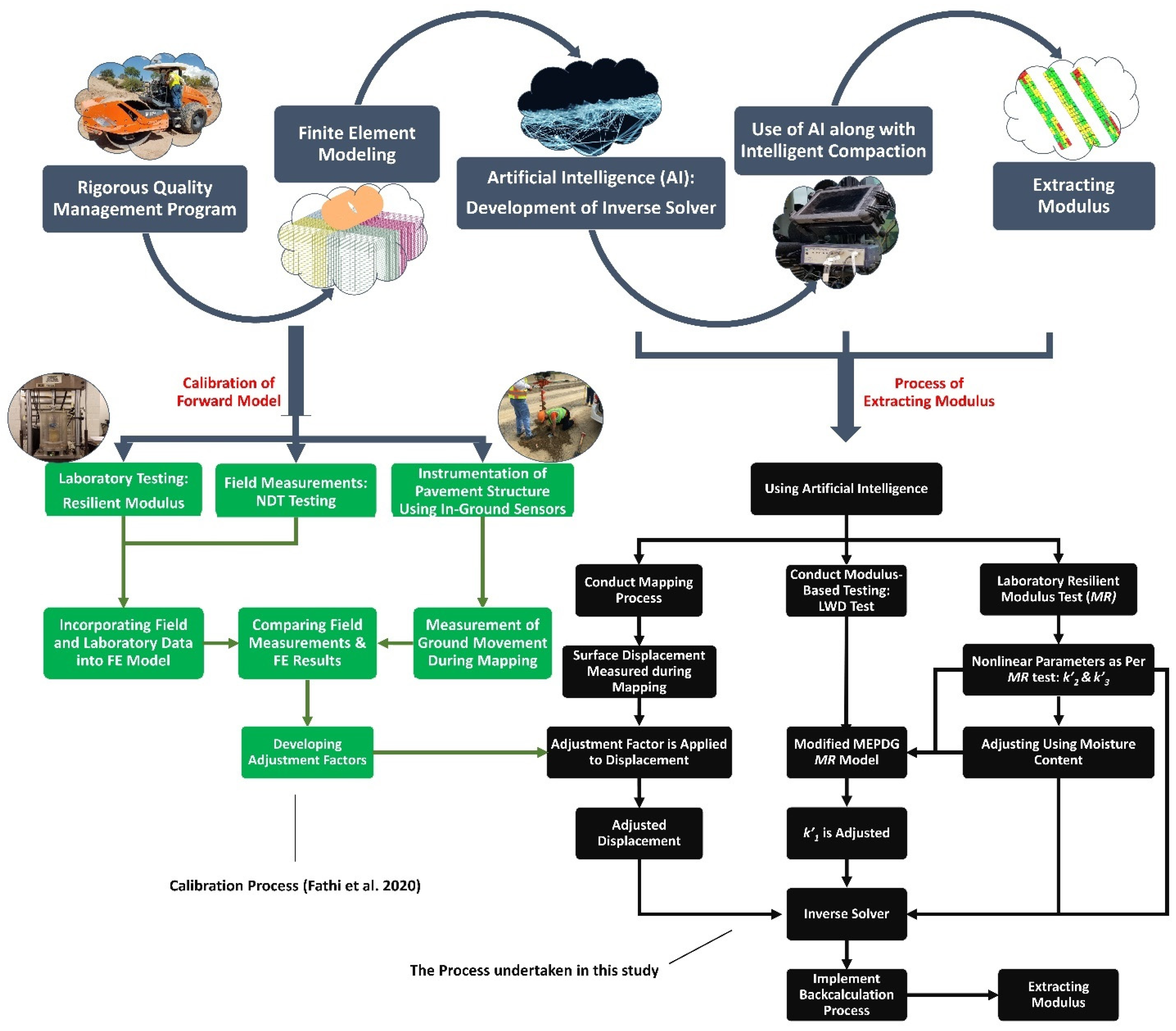
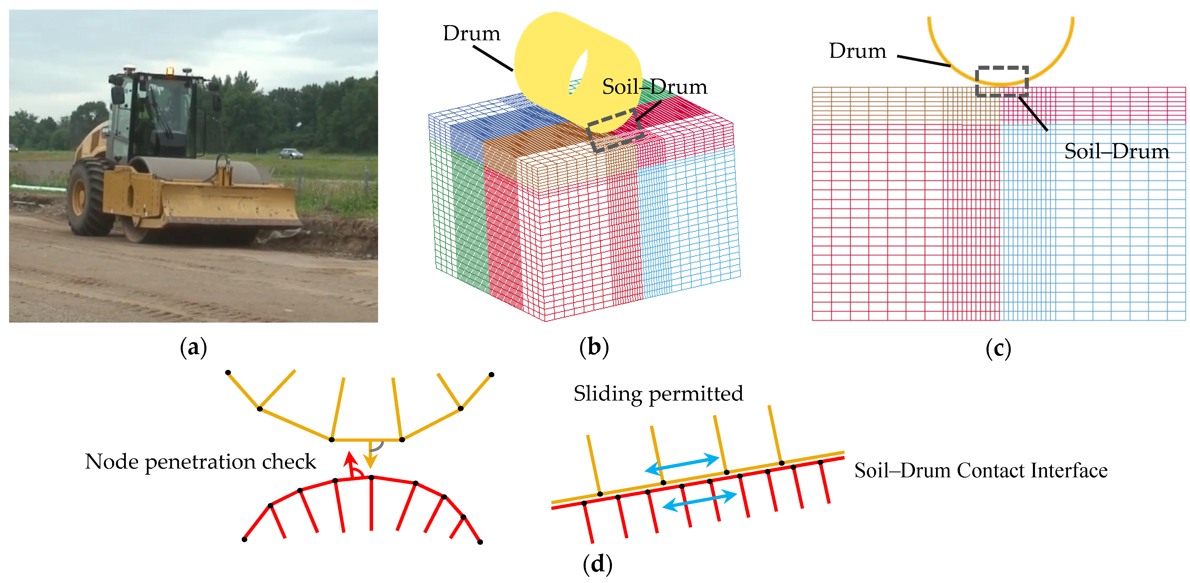
- Three-dimensional FE models simulating the proof-mapping process of an IC-roller on compacted materials were developed and utilized to develop a database with a wide range of pavement materials and structures. The FE models incorporated a nonlinear constitutive model to simulate the behavior of geomaterials under the imposed drum loads and a contact model to simulate the drum decoupling from the soil surface, which is similar to what is observed in the field.
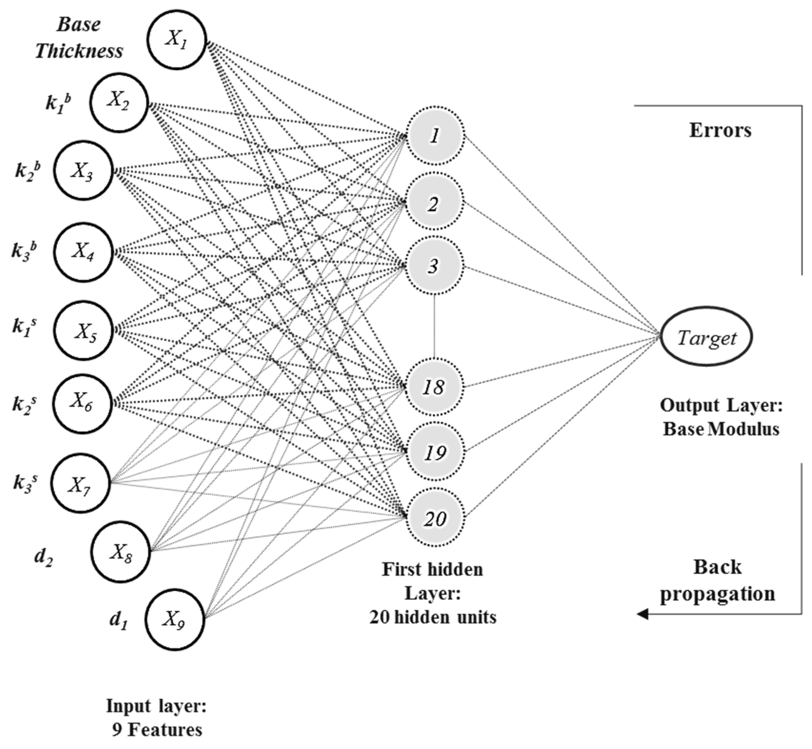
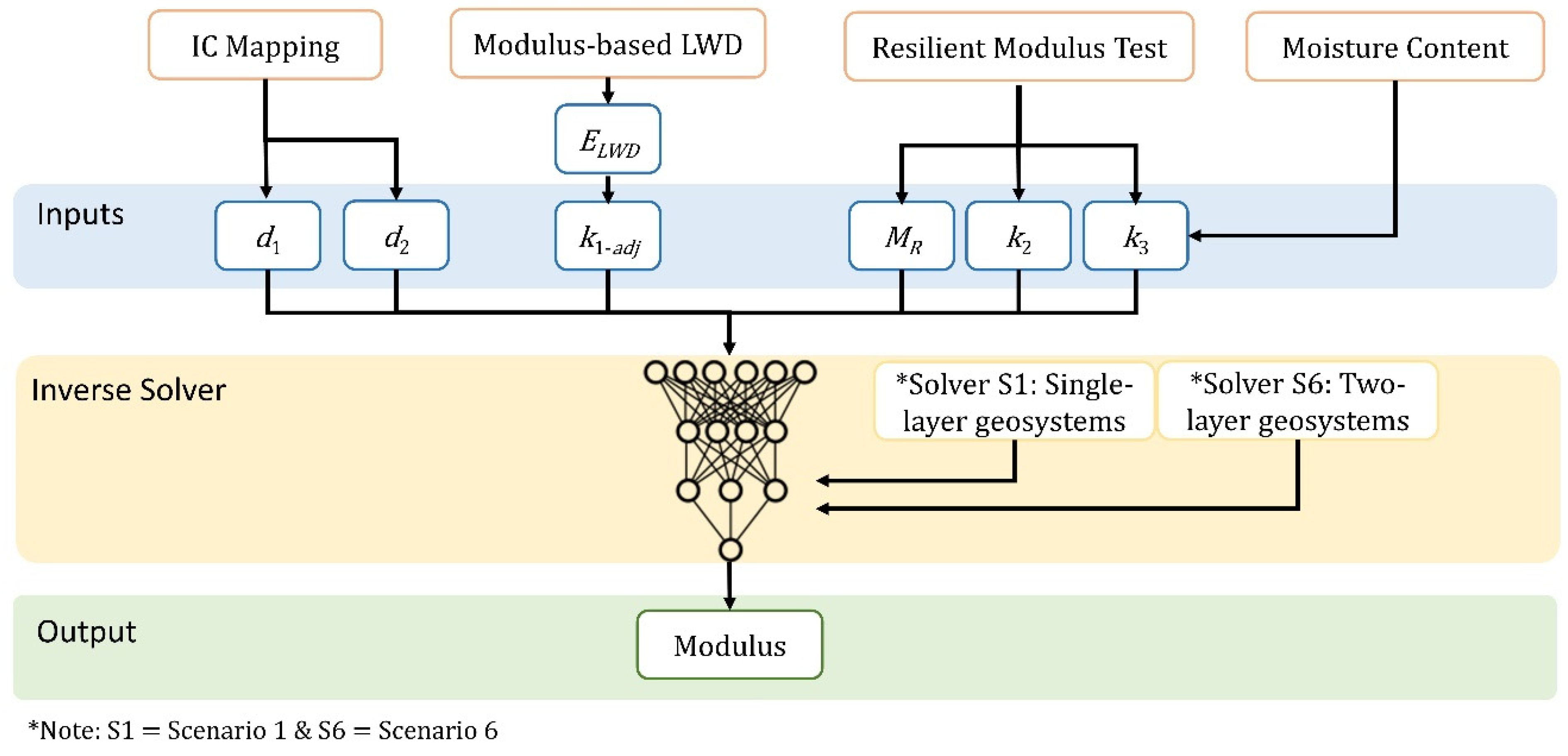
- A comprehensive database of pavement responses under the imposed drum loads for one- and two-layered systems was assembled and used to develop various inverse solvers using artificial neural networks for the prediction of the moduli of the subgrade and the base layered materials.
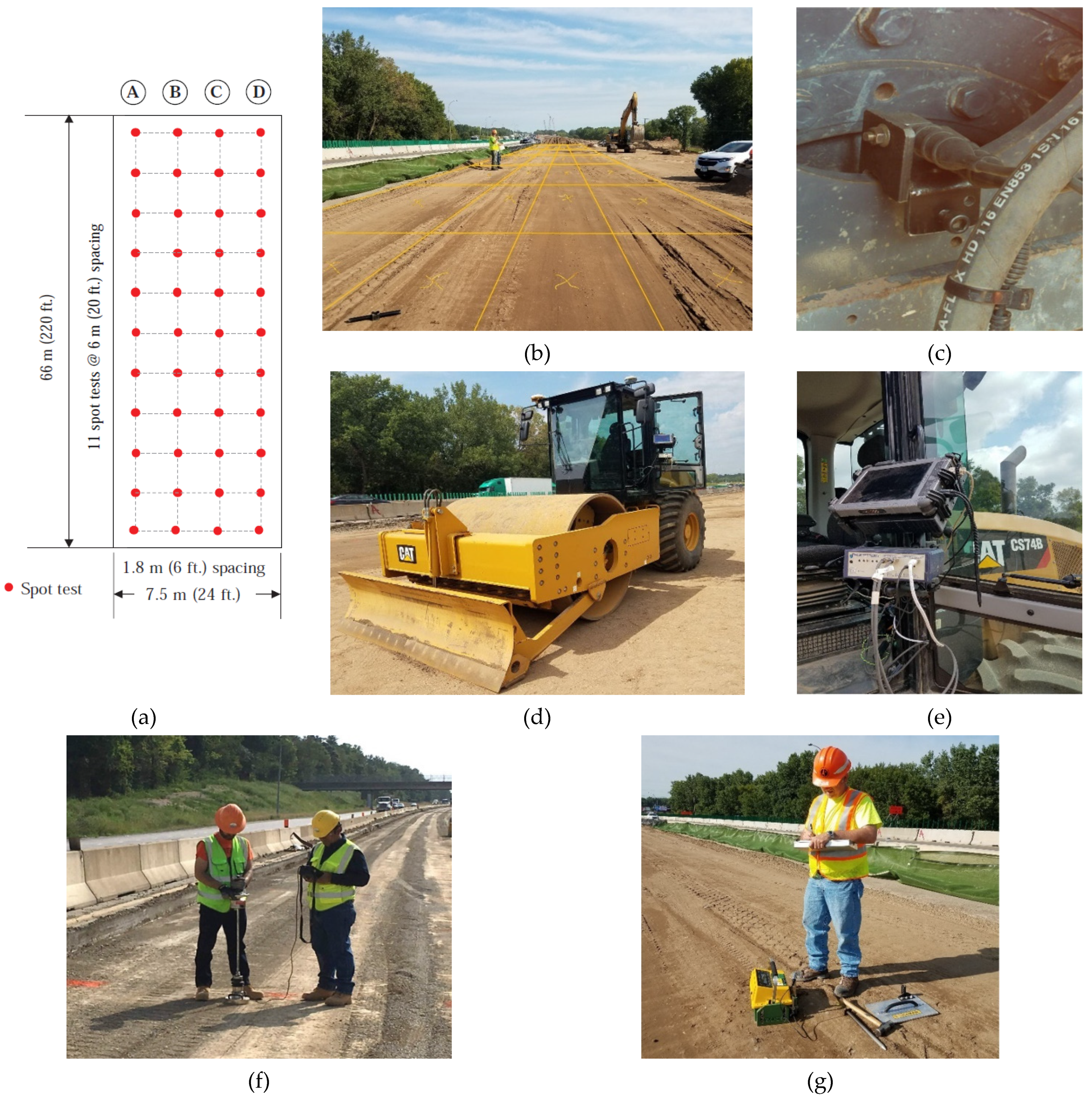
- In addition to the developed forward and inverse models, eight test sites, including single- (subgrade only) and two-layer (subgrade and base course layer) geosystems, were instrumented using in-ground sensors to measure the ground vibrations induced by the roller during the mapping process. Four test sites were used for the calibration of the forward models and inverse solvers. The other four construction sites were utilized for the further evaluation and validation of the proposed approach.
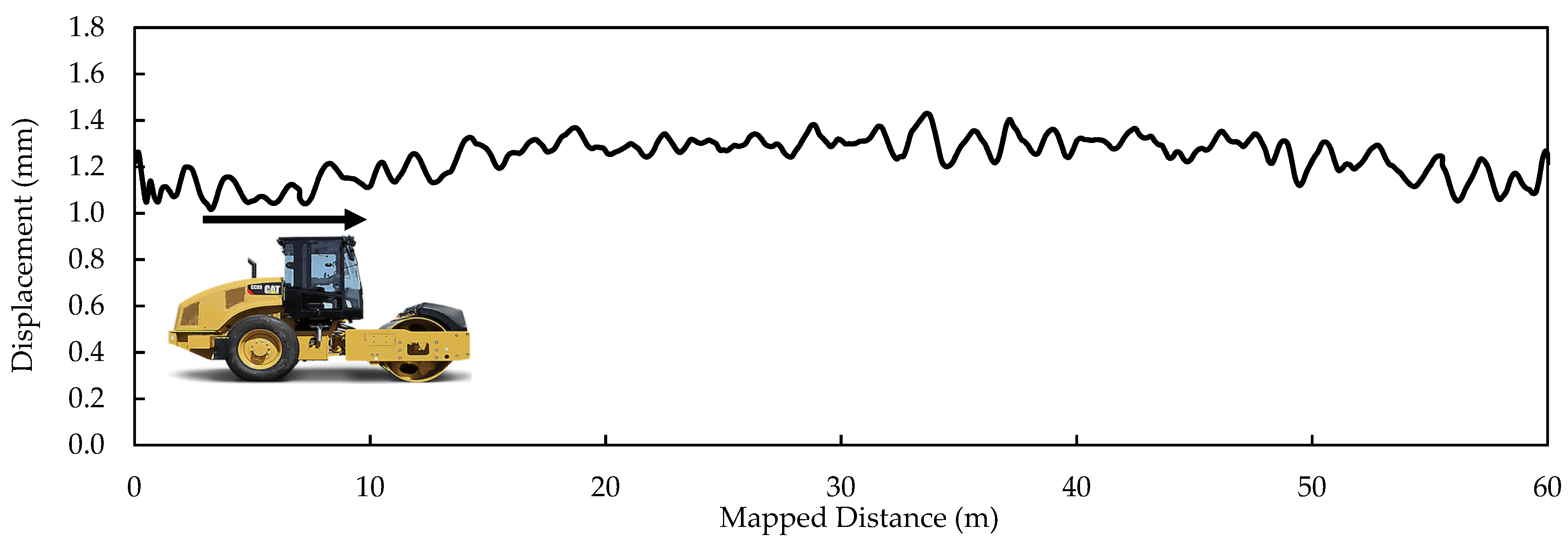
- Rollers were instrumented using drum-mounted accelerometers to measure the pavement response, and omega arithmetic was employed to measure displacement during mapping, which was used as one of the inputs to the inverse models.
- Along with an IC testing program at the constructed sites, modulus-based testing with LWD and the measurement of the moisture at the time of compaction with NDG and oven testing were implemented on the compacted geomaterials.
- Laboratory tests including index tests as well as resilient modulus tests were also conducted on sampled materials collected from the test sites to ensure that comprehensive information existed for the development and assessment of the proposed approach.
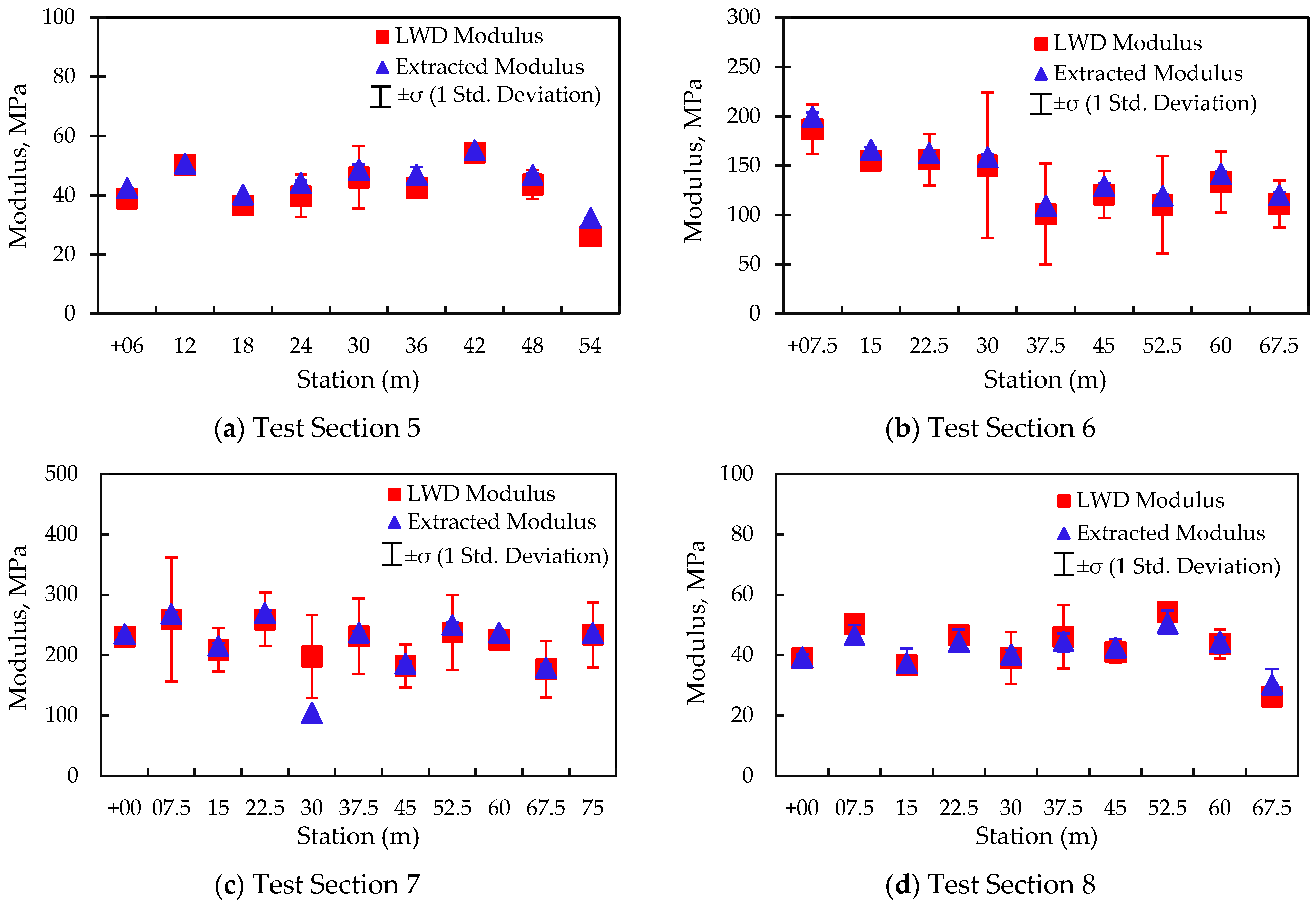
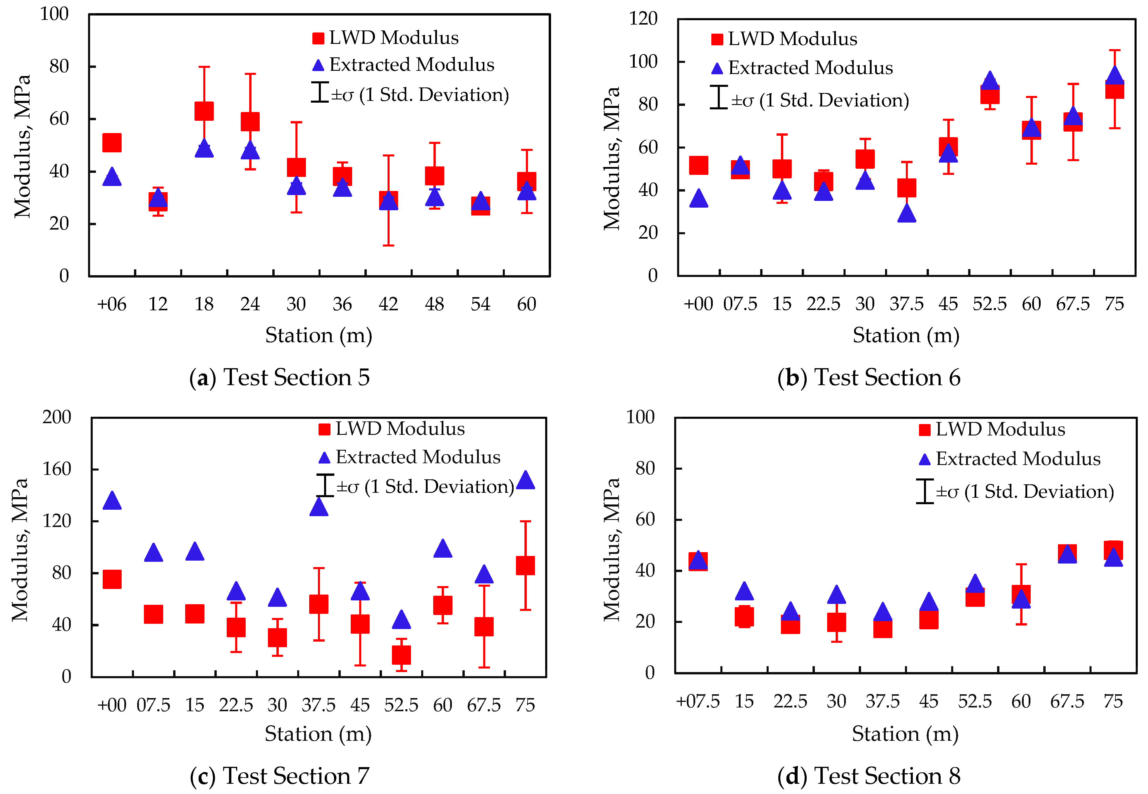
- The constructed inverse solvers were capable of extracting moduli in single- and two-layered systems. For t two-layer systems in particular, the modulus of the top layer can be extracted when the layer underneath, is pre-mapped and when the thickness information for the top layer is available.
- More accurate moduli are obtained from the inverse solvers when modulus-based field measurements using LWD and resilient modulus testing are incorporated as part of the quality management program.
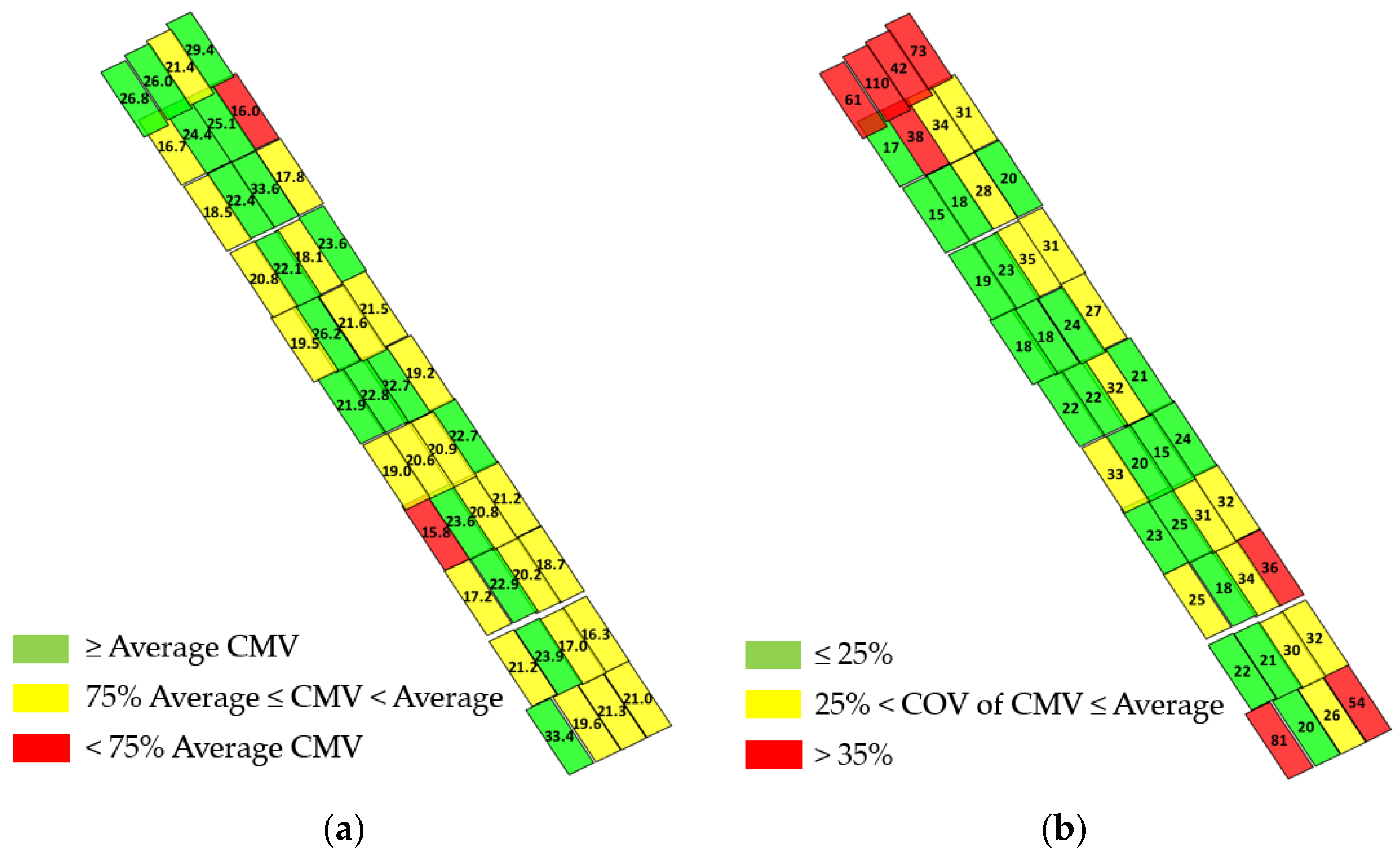
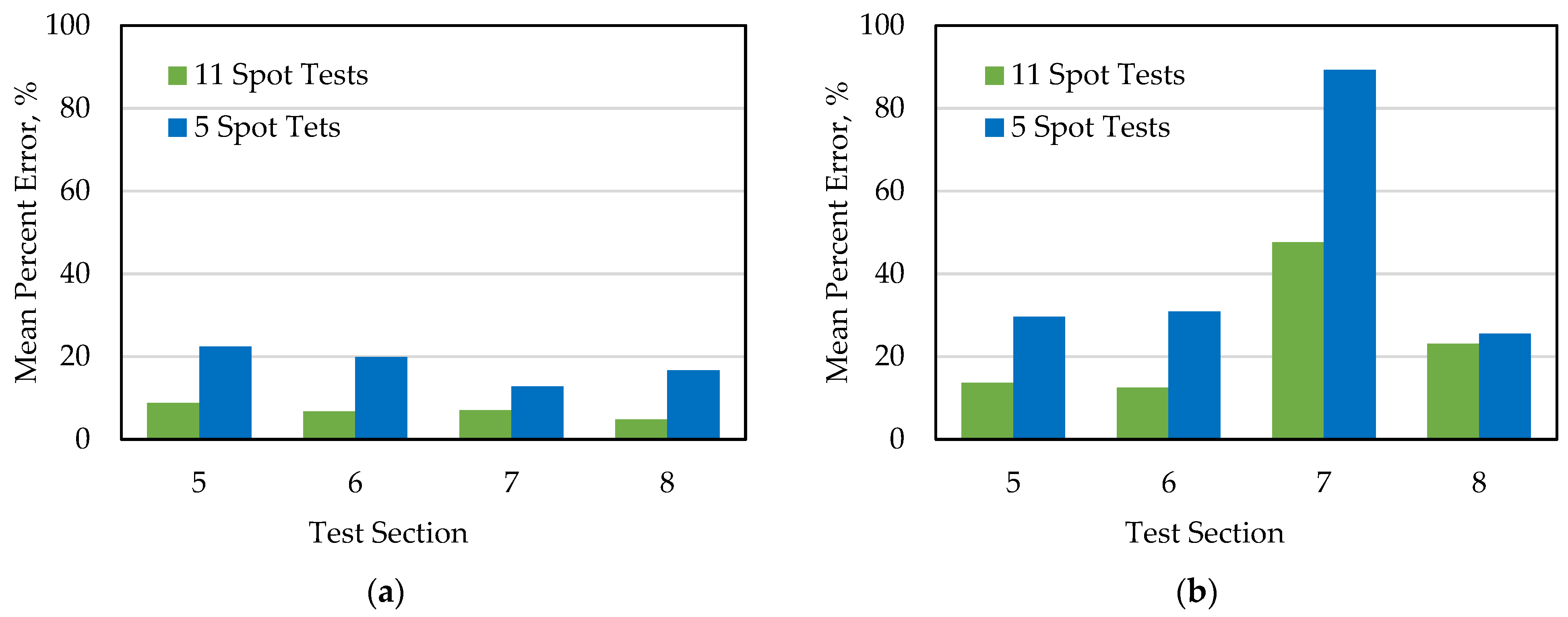
- The proposed approach was found to be favorable for the estimation of the moduli of compacted soils when modulus-based testing was conducted in sublots exhibiting moderate nonuniformity, i.e., COV of ICMV ≤ 35%. The compaction uniformity plays a key role in the retrieval of the moduli of geomaterials with certainty.
- When compaction uniformity is not achieved, an LWD spot test cannot appropriately represent the compaction quality for a sublot with an approximate size of 45 m2. The impact of not excluding sublots with high non-uniformity leads the solver to estimate the moduli with poor accuracy.
- The selection of 10% of the available sublots can yield modulus estimations within a 25% error, a value that is still within the variability of the properties of compacted geomaterials observed under the best construction practices.
- Modulus-based maps can be generated utilizing the proposed approach, and the accelerometer-based measurements collected during the mapping of the lot using various line passes to cover 100% of the lot.
Author Contributions
Funding
Institutional Review Board Statement
Informed Consent Statement
Data Availability Statement
Acknowledgments
Conflicts of Interest
References
- Siekmeier, J.; Pinta, C.; Merth, S.; Jensen, J.; Davich, P.; Camargo, F.F.; Beyer, M. Using the Dynamic Cone Penetrometer and Light Weight Deflectometer for Construction Quality Assurance; Report No. MN/RC 2009-12; Office of Materials and Road Research, Minnesota Department of Transportation: St. Paul, MN, USA, 2009. [Google Scholar]
- Vennapusa, P.K.; White, D.J. Comparison of Light Weight Deflectometer Measurements for Pavement Foundation Materials. Geotech. Test. J. 2009, 32, 1–13. [Google Scholar] [CrossRef]
- Mooney, M.A.; Rinehart, R.V.; Facas, N.W.; Musimbi, O.M.; White, D.J.; Vennapusa, P.K.R. NCHRP Research Report 676: Intelligent Soil Compaction Systems; Transportation Research Board of the National Academies: Washington, DC, USA, 2010. [Google Scholar] [CrossRef]
- Nazarian, S.; Mazari, M.; Abdallah, I.N.; Puppala, A.J.; Mohammad, L.N.; Abu-Farsakh, M.Y. Modulus-Based Construction Specification for Compaction of Earthwork and Unbound Aggregate; Transportation Research Board, The National Academies Press: Washington, DC, USA, 2010. [Google Scholar] [CrossRef]
- Ganju, E.; Kim, H.; Prezzi, M.; Salgado, R.; Siddiki, N.Z. Quality Assurance and Quality Control of Subgrade Compaction Using the Dynamic Cone Penetrometer. Int. J. Pavement Eng. 2018, 19, 966–975. [Google Scholar] [CrossRef]
- Tirado, C.; Rocha, S.; Fathi, A.; Mazari, M.; Nazarian, S. Deflection-Based Field Testing for Quality Management of Earthwork; Report No. FHWA/TX-19/0-6903-1; Center for Transportation Infrastructure System, The University of Texas at El Paso: El Paso, TX, USA, 2019. [Google Scholar]
- Nazarian, S.; Fathi, A.; Tirado, C.; Kreinovich, V.; Rocha, S.; Mazari, M. NCHRP Research Report 933: Evaluating Mechanical Properties of Earth Material during Intelligent Compaction; National Academies of Sciences, Engineering, and Medicine, The National Academies Press: Washington, DC, USA, 2020. [Google Scholar] [CrossRef]
- Nieves Torres, A.; Arasteh, M. Intelligent Compaction Measurement Values (ICMV)—A Road Map; Technical Brief, FHWA-HIF-17-046; Federal Highway Administration: Washington, DC, USA, 2017. [Google Scholar]
- Tirado, C.; Fathi, A.; Rocha, S.; Mazari, M.; Nazarian, S. Integrating Intelligent Compaction Technology and Modulus-Based Testing for Design Verification. Proc. Inst. Civ. Eng. Geotech. Eng. 2020, 173, 327–338. [Google Scholar] [CrossRef]
- Anderegg, R.; Kaufmann, K. Intelligent Compaction with Vibratory Rollers: Feedback Control Systems in Automatic Compaction and Compaction Control. Transp. Res. Rec. J. Transp. Res. Board 2004, 1868, 124–134. [Google Scholar] [CrossRef]
- White, D.J.; Thompson, M.J. Relationships between in Situ and Roller-Integrated Compaction Measurements for Granular Soils. J. Geotech. Geoenviron. Eng. 2008, 134, 1763–1770. [Google Scholar] [CrossRef]
- Gallivan, V.L.; Chang, G.K.; Horan, D.R. Intelligent Compaction for Improving Roadway Construction. In Emerging Technologies for Material, Design, Rehabilitation, and Inspection of Roadway Pavements 2011, Proceeding of the GeoHunan International Conference 2011, Hunan, China, 9–11 June 2011; ASCE: Hunan, China, 2011; pp. 117–124. [Google Scholar] [CrossRef]
- Meehan, C.L.; Tehrani, F.S.; Vahedifard, F. A Comparison of Density-based and Modulus-Based in Situ Test Measurements for Compaction Control. Geotech. Test. J. 2012, 35, 387–399. [Google Scholar] [CrossRef] [Green Version]
- Fathi, A.; Tirado, C.; Mazari, M.; Rocha, S.; Nazarian, S. Correlating Continuous Compaction Control Measurements to In Situ Modulus-Based Testing for Quality Assessment of Compacted Geomaterials. In Proceedings of the International Conference on Information Technology in Geo-Engineering 2019, Guimarães, Portugal, 29 September–2 October 2019; Correia, A., Tinoco, J., Cortez, P., Lamas, L., Eds.; Springer: Cham, Switzerland, 2020; pp. 585–595. [Google Scholar] [CrossRef]
- Barman, M.; Nazari, M.; Imran, S.A.; Commuri, S.; Zaman, M.; Beainy, F.; Singh, D. Quality Control of Subgrade Soil using Intelligent Compaction. Innov. Infrastruct. Solut. 2016, 1, 23. [Google Scholar] [CrossRef] [Green Version]
- Lemus, L.; Fathi, A.; Beltran, J.; Gholami, A.; Tirado, C.; Mazari, M.; Nazarian, S. Geospatial Relationship of Intelligent Compaction Measurement Values with In Situ Testing for Quality Assessment of Geomaterials. In Airfield and Highway Pavements, Proceedings of the International Conference on Transportation and Development 2018, Pittsburgh, PA, USA, 15–18 July 2018; ASCE: Reston, VA, USA, 2018; pp. 293–301. [Google Scholar] [CrossRef]
- Baker, W.J., III; Meehan, C.L. Continuous Compaction Control Measurements for Quality Assurance in Conjunction with Light Weight Deflectometer Target Modulus Values. In Proceedings of the Geo-Congress 2020: Modeling, Geomaterials, and Site Characterization, Minneapolis, MN, USA, 25–28 February 2020; ASCE: Reston, VA, USA, 2020; pp. 368–376. [Google Scholar] [CrossRef]
- Lundberg, V.G. Elastische berührung zweier halbräume. Forschung auf dem Gebiet des Ingenieurwesens A 1939, 10, 201–211. [Google Scholar] [CrossRef]
- Kröber, W. Untersuchung der Dynamischen Vorgänge bei der Vibrationsverdichtung von Böden. Ph.D. Thesis, Technische Universität München (TUM), Munich, Germany, 1998. [Google Scholar]
- Floss, R.; Kröber, W.; Wallrath, W. Dynamische Bodensteifigkeit als Qualitätskriterium für die Bodenverdichtung (Dynamic Soil Stiffness as a Quality Criterion for Soil Compaction). In Proceedings of the 4. Internationales Symposium Technik und Technologie des Verkehrswegebaus (4th International Symposium and Technology Series of Transportation Infrastructures), Munich, Germany, 4–6 April 2001; BAUMA: Munich, Germany, 2001. [Google Scholar]
- Sandström, A.J.; Pettersson, C.B. Intelligent Systems for QA/QC in Soil Compaction. In Proceedings of the 83rd Annual Transportation Research Board Meeting, Washington, DC, USA, 11–15 January 2004; Transportation Research Board: Washington, DC, USA, 2004; pp. 11–14. [Google Scholar]
- Mooney, M.A.; Facas, N.W. NCHRP IDEA Project 145: Extraction of Layer Properties from Intelligent Compaction Data; Transportation Research Board: Washington, DC, USA, 2013. [Google Scholar]
- White, D.J.; Vennapusa, P.; Tutumluer, E.; Moaveni, M. Mechanistic Assessment of Layered Pavement Foundation System Using Validated Intelligent Compaction Measurements. In Proceedings of the 8th International Conference on Case Histories in Geotechnical Engineering (Geo-Congress 2019), Philadelphia, PA, USA, 24–27 March 2019; ASCE: Reston, VA, USA, 2019; pp. 421–429. [Google Scholar] [CrossRef]
- White, D.J.; Vennapusa, P.; Roesler, J.R.; Vavrik, W. Plate Load Testing on Layered Pavement Foundation System to Characterize Mechanistic Parameters. In Proceedings of the 8th International Conference on Case Histories in Geotechnical Engineering (Geo-Congress 2019), Philadelphia, PA, USA, 24–27 March 2019; ASCE: Reston, VA, USA, 2019; pp. 214–226. [Google Scholar] [CrossRef]
- Rahman, F.; Hossain, M.; Hunt, M.M.; Romanoschi, S.A. Soil Stiffness Evaluation for Compaction Control of Cohesionless Embankments. Geotech. Test. J. 2018, 31, 442–451. [Google Scholar] [CrossRef]
- Ooi, P.S.; Archilla, A.R.; Sandefur, K.G. Resilient Modulus Models for Compacted Cohesive Soils. Transp. Res. Rec. J. Transp. Res. Board 2004, 1874, 115–124. [Google Scholar] [CrossRef]
- Velasquez, R.; Hoegh, K.; Yut, I.; Funk, N.; Cochran, G.; Marasteanu, M.; Khazanovich, L. Implementation of the MEPDG for New and Rehabilitated Pavement Structures for Design of Concrete and Asphalt Pavements in Minnesota; Report No. MN/RC 2009-06; University of Minnesota: Minneapolis, MN, USA.
- Werbos, P. Beyond Regression: New Tools for Prediction and Analysis in the Behavioral Sciences. Ph.D. Thesis, Harvard University, Cambridge, MA, USA, 1974. [Google Scholar]
- Ilonen, J.; Kamarainen, J.K.; Lampinen, J. Differential Evolution Training Algorithm for Feed-forward Neural Networks. Neural Process. Lett. 2003, 17, 93–105. [Google Scholar] [CrossRef]
- Hastie, T.; Tibshirani, R.; Friedman, J. The Elements of Statistical Learning: Data Mining, Inference, and Prediction; Springer Science & Business Media: New York, NY, USA, 2009. [Google Scholar] [CrossRef]
- Fathi, A.; Tirado, C.; Rocha, S.; Mazari, M.; Nazarian, S. Incorporating Calibrated Numerical Models in Estimating Moduli of Compacted Geomaterials from Integrated Intelligent Compaction Measurements and Laboratory Testing. Transp. Res. Rec. J. Transp. Res. Board 2020, 2674, 75–88. [Google Scholar] [CrossRef]
- Mercer, C. Acceleration, Velocity and Displacement Spectra-Omega Arithmetic. Prosig Signal Process. Tutor. 2006, 1, 1–8. [Google Scholar]
- Mazari, M.; Navarro, E.; Abdallah, I.; Nazarian, S. Comparison of Numerical and Experimental Responses of Pavement Systems using Various Resilient Modulus Models. Soils Found. 2014, 54, 36–44. [Google Scholar] [CrossRef] [Green Version]


| Pavement Properties | Range of Values |
|---|---|
| k′1 | 100–3000 |
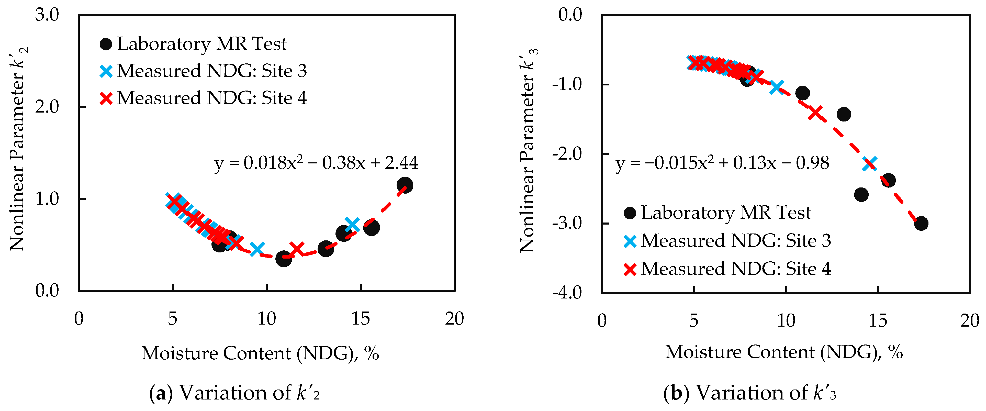
| k′2 | 0–3.0 |
| k′3 | −4.0–0 |
| Poisson’s Ratio, ν | 0.35 |
| Operating Parameter | Symbol | Range of Values | Baseline Roller Values |
|---|---|---|---|
| Width of drum | L | 1.0–2.0 m | 2.0 m |
| Diameter of drum | d | 0.5 m–1.5 m | 1.5 m |
| Mass of drum | md | 750–9000 kg | 6000 kg |
| Weight of drum | mdg | 7500–88,000 N | 58,840 N |
| Mass-eccentricity | m0e0 | 1.0–5.6 kg·m | 5.36 kg·m |
| Centrifugal force | Fev | 15–170 kN | 170 kN |
| Frequency | f | 20–60 Hz | 28 Hz |
| Rotational Frequency | Ω | 125–380 rad/s | 176 rad/s |
| Operating speed | v | 0.9 m/s | 0.9 m/s |
| Geosystem | Scenario | Input Parameters | Coefficient of Determination, R2 | Standard Error of the Estimate, SEE (ksi) | Recommendation for Implementation 1 | Target |
|---|---|---|---|---|---|---|
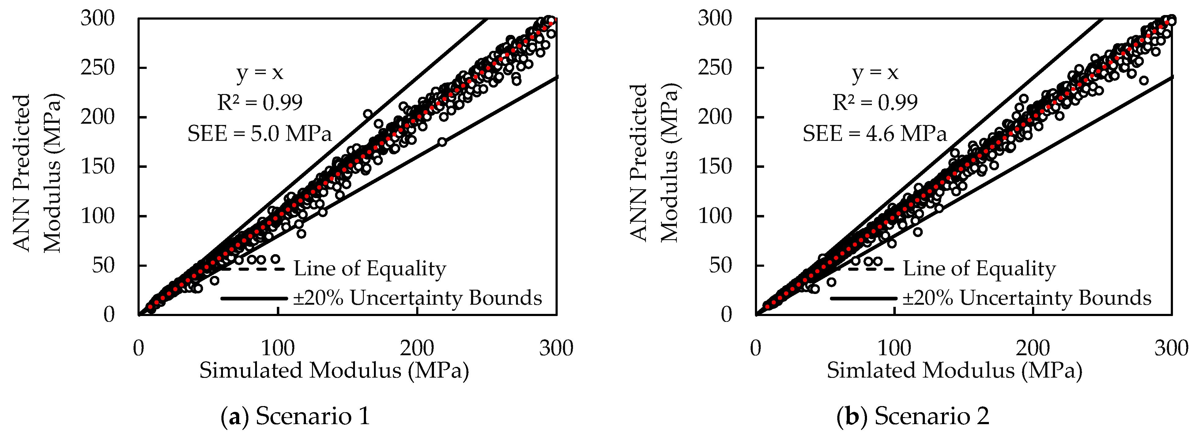
| One layer | 1 | h, k′1s, k′2s, k′3s, d1 | 0.99 | 5.0 | High | Subgrade Modulus, ESUBG |
| 2 | h, k′1s, k′2s, k′3s, d1, MRSUBG-Rep | 0.99 | 4.6 | Moderate | ||
| Two-layer | 3 | h, k′2b, k′3b, d2, d1 | 0.77 | 29.4 | Low | Base Modulus, EBASE |
| 4 | h, k′2b, k′3b, d2, ESUBG | 0.70 | 31.6 | Low | ||
| 5 | h, k′2b, k′3b, d2, MRSUBG-Rep | 0.76 | 29.5 | Low | ||
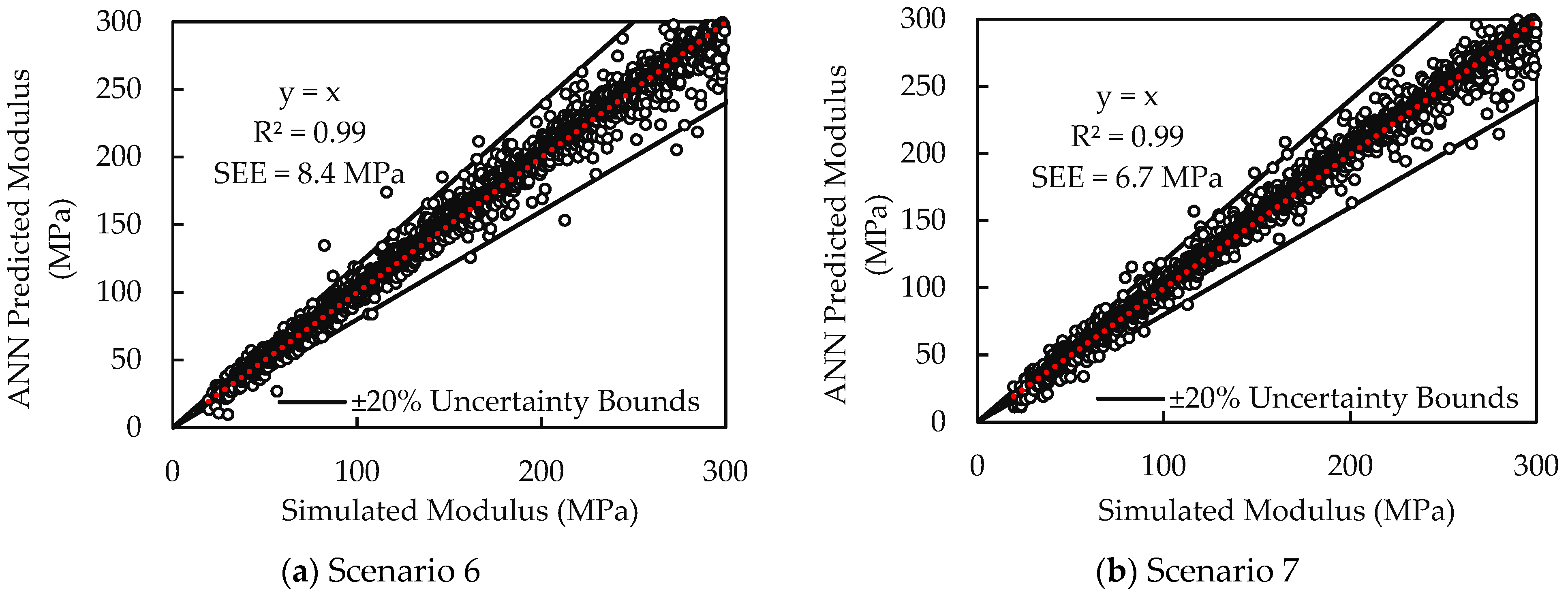
| 6 | h, k′1b, k′2b, k′3b, d2, d1 | 0.99 | 8.4 | High | ||
| 7 | h, k′1s, k′2s, k′3s, k′1b, k′2b, k′3b, d2, d1 | 0.99 | 6.7 | Moderate |
| Test Section | Layer | USCS Classification | Optimum Moisture Content, OMC 1 (%) | Maximum Dry Density (MDD) (kg/m3) | Resilient Modulus at OMC (MPa) |
|---|---|---|---|---|---|
| 1 | Sand subgrade (existing) | SP-SM | 6.5 | 1342 | 77.9 |
| 300 mm coarse Class 5Q aggregate base coarse recycled concrete | GW | 10.5 | 1962 | 128.7 | |
| 2 | Sand subgrade (existing) | SP-SM | 6.5 | 1342 | 77.9 |
| 300 mm fine Class 5 aggregate base fine recycled concrete | SP | 10.9 | 1922 | 126.2 | |
| 3 | Clay loam (A-6) prepared subgrade | CL | 14.4 | 1897 | 59.3 |
| 300 mm Class 6 aggregate base limestone | GW | 6.6 | 2284 | 97.9 | |
| 4 | Clay loam (A-6) prepared subgrade | CL | 14.4 | 1897 | 59.3 |
| 300 mm Class 6 aggregate base recycled concrete and asphalt | GP | 10.5 | 1969 | 117.2 |
| Vendor/Manufacturer | Model | Drum Mass (kg) | Operating Amplitude (mm) | Operating Frequency (Hz) | Centrifugal Force (kN) |
|---|---|---|---|---|---|
| Caterpillar | CS74B | 5153 | 0.99 | 28.3 | 160 |
| Test Section | Layer | Resilient Modulus at OMC 1 (MPa) | Extracted Nonlinear Parameters from Resilient Modulus Tests | Average LWD Modulus, ELWD 2 (MPa) | ||
|---|---|---|---|---|---|---|
| k′1 | k′2 | k′3 | ||||
| 1 | Sand subgrade (existing) | 77.9 | 335 | 1.6 | −0.6 | 29 |
| 300 mm coarse Class 5Q aggregate base coarse recycled concrete | 128.7 | 512 | 0.8 | −0.1 | 117 | |
| 2 | Sand subgrade (existing) | 77.9 | 335 | 1.6 | −0.6 | 36 |
| 300 mm fine Class 5 aggregate base fine recycled concrete | 126.2 | 484 | 0.9 | −0.1 | 193 | |
| 3 | Clay loam (A-6) prepared subgrade | 59.3 | 649 | 0.6 | −2.6 | 43 |
| 300 mm Class 6 aggregate base limestone | 97.9 | 500 | 0.6 | −0.1 | 138 | |
| 4 | Clay loam (A-6) prepared subgrade | 59.3 | 649 | 0.6 | −2.6 | 26.3 |
| 300 mm Class 6 aggregate base recycled concrete and asphalt | 117.2 | 408 | 0.9 | −0.1 | 134 | |
| Site | Length (m) | Layer | USCS Classification | Optimum Moisture Content 1 (%) | Maximum Dry Density, (kg/m3) | Roller Vendor/Model |
|---|---|---|---|---|---|---|
| 5 | 66 | Embankment | CL | 13.8 | 1853 | Hamm H11ix |
| 300 mm subgrade | CL | 17.1 | 1802 | |||
| 6 | 75 | Subgrade | SP | 7.1 | 2142 | Caterpillar CS74B |
| 300 mm subbase | SP | 7.1 | 2142 | |||
| 7 | 75 | Cement-treated subgrade (4% cement) | - | - | - | Caterpillar CS74B |
| 150 mm unbound aggregate base course | GW | 6.5 | 2289 | |||
| 8 | 66 | Embankment | CL | 13.8 | 1899 | Volvo SD75 |
| 300 mm subgrade | CL | 13.8 | 1899 |
| Vendor/Manufacturer | Caterpillar | Hamm/Wirtgen | Volvo |
|---|---|---|---|
| Model |  CS74B |  H11 ix |  SD75 |
| Drum Width (m) | 2.1 | 2.1 | 1.7 |
| Drum Mass (kg) | 5153 | 5890 | 3610 |
| Operating Amplitude (mm) | 0.99 | 0.84 | 1.20 |
| Operating Frequency (Hz) | 28.3 | 30 | 30 |
| Centrifugal Force (kN) | 160 | 136 | 121 |
| Test Section | Resilient Modulus at OMC 1 (MPa) | Nonlinear Parameters from Resilient Modulus Model 2 | Average in situ LWD Modulus, ELWD (MPa) | Adjusted Nonlinear Parameter k′1-adj 3 | Surface Displacement (mm) | ||
|---|---|---|---|---|---|---|---|
| k′2 | k′3 | Layer 1 d1 | Layer 2 d2 | ||||
| Single Layer Systems | |||||||
| 5 | 40 | 1.57 | −2.04 | 39 | 217 | 1.07 | - |
| 6 | 115 | 1.69 | −2.16 | 130 | 598 | 1.26 | - |
| 7 | 230 | 0.61 | −0.05 | 231 | 1581 | 1.08 | - |
| 8 | 37 | 1.76 | −2.60 | 40 | 213 | 1.07 | - |
| Two-Layer Systems | |||||||
| 5 | 39 | 1.24 | −3.00 | 40 | 313 | 1.07 | 1.11 |
| 6 | 51 | 1.69 | −2.16 | 58 | 267 | 1.26 | 1.52 |
| 7 | 103 | 0.57 | −0.05 | 91 | 329 | 1.08 | 1.05 |
| 8 | 37 | 1.76 | −2.60 | 29 | 214 | 1.07 | 1.11 |
Publisher’s Note: MDPI stays neutral with regard to jurisdictional claims in published maps and institutional affiliations. |
© 2021 by the authors. Licensee MDPI, Basel, Switzerland. This article is an open access article distributed under the terms and conditions of the Creative Commons Attribution (CC BY) license (https://creativecommons.org/licenses/by/4.0/).
Share and Cite
Fathi, A.; Tirado, C.; Rocha, S.; Mazari, M.; Nazarian, S. A Machine-Learning Approach for Extracting Modulus of Compacted Unbound Aggregate Base and Subgrade Materials Using Intelligent Compaction Technology. Infrastructures 2021, 6, 142. https://0-doi-org.brum.beds.ac.uk/10.3390/infrastructures6100142
Fathi A, Tirado C, Rocha S, Mazari M, Nazarian S. A Machine-Learning Approach for Extracting Modulus of Compacted Unbound Aggregate Base and Subgrade Materials Using Intelligent Compaction Technology. Infrastructures. 2021; 6(10):142. https://0-doi-org.brum.beds.ac.uk/10.3390/infrastructures6100142
Chicago/Turabian StyleFathi, Aria, Cesar Tirado, Sergio Rocha, Mehran Mazari, and Soheil Nazarian. 2021. "A Machine-Learning Approach for Extracting Modulus of Compacted Unbound Aggregate Base and Subgrade Materials Using Intelligent Compaction Technology" Infrastructures 6, no. 10: 142. https://0-doi-org.brum.beds.ac.uk/10.3390/infrastructures6100142