
A Machine Learning Framework for Predicting Bridge Defect Detection Cost

Department of Bridge and Tunnel Engineering, School of Civil Engineering, Southwest Jiaotong University, No. 111, North 1st Section of Second Ring Road, Jinniu District, Chengdu 610031, China
*
Author to whom correspondence should be addressed.
Infrastructures 2021, 6(11), 152; https://0-doi-org.brum.beds.ac.uk/10.3390/infrastructures6110152
Submission received: 18 September 2021
/
Revised: 12 October 2021
/
Accepted: 19 October 2021
/
Published: 23 October 2021
Abstract
:Evaluating the cost of detecting bridge defects is a difficult task, but one that is vital to the lifecycle cost analysis of bridges. In this study, a detection cost sample database was established based on practical engineering data, and a bridge defect detection cost prediction model and software were developed using machine learning. First, the random forest method was adopted to evaluate the importance of the seven main factors affecting the detection cost. The most important indicators were selected, and the recent GDP growth rate was employed to account for the impact of social and economic developments on the detection cost. Combining a genetic algorithm with a multilayer neural network, a detection cost prediction model was established. The predictions given by this model were found to have an average relative error of 3.41%. Finally, an intelligent prediction software for bridge defect detection costs was established, providing a reliable reference for bridge lifecycle cost analysis and the evaluation of defect detection costs during the operation period.
1. Introduction
The service life of bridge structures is typically several decades and possibly more than a century. To guarantee the safety, reliability, and performance of bridges, bridge managers conduct activities such as monitoring, defect detection, and maintenance [1]. In examining the sustainability of bridge construction and the efficiency of the investment cost, it is important to balance the operating costs incurred by the various management activities during the service period and the construction costs of the bridge. Choosing design schemes based on the construction cost alone does not reflect future funding demand, nor is it consistent with the direction of sustainable development [2]. Studying the lifecycle cost of a bridge can provide huge long-term economic benefits, identify various future expenditures, and provide a scientific basis for economic decisions [3]. Due to the uncertainty of the operating costs, effective cost estimation and prediction methods are needed to evaluate the overall cost of different bridges over their service life, as these allow managers to make the most appropriate decisions [4]. Bridge operating costs are mainly composed of defect detection costs, maintenance costs, and user costs [5]. Therefore, the efficient and accurate prediction of defect detection costs is helpful to the calculation and control of operating costs.
A scientific evaluation of the operating costs of a bridge should account for the bridge condition, the bridge location, and the time of management activities, and allocate appropriate management resources and funds [6]. Studying the operating costs mostly focused on allocation and optimization, while the research on operating cost prediction is less and mostly focused on the field of maintenance costs. For example, maintenance cost estimation based on deterioration model [7], bridge maintenance cost allocation based on prioritization indexes [8], routine maintenance cost prediction based on linear regression and time series analysis [9], bridge maintenance cost optimization based on system reliability analysis and genetic algorithm [10]. At present, there are few studies on the bridge defect detection cost, and the cost is usually regarded as the product of the fixed detection times and the unit detection cost. The unit detection cost is usually appointed as a fixed value or the calculation result of a simple empirical formula. Most of the studies ignore the possible changes in the defect detection cost over time, nor are they consistent with the actual situation [11,12,13]. The values in these studies have not been effectively verified by engineering data, and therefore, it is difficult to guarantee their reliability.
Accurate prediction of the cost of bridge defect detection is of great significance to the analysis of bridge life cycle cost. Machine learning has obvious advantages and good results in solving these problems. There are several advantages of utilizing machine learning methods for predicting bridge defect detection cost. The algorithms efficiently learn the underlying relationships between input indexes and bridge defect detection costs. Furthermore, they have the potential to identify some important but less intuitive hidden influencing factors. These machine learning algorithms are convenient to implement and computationally efficient. Finally, they allow model updating once new information from the cost of bridge defect detection becomes available. Machine learning methods have been successfully applied in different aspects of structural engineering. Examples of such applications include classification of in-plane failure modes for reinforced concrete frames with infills [14]; structural collapse modes classification [15]; post-earthquake structural safety assessment [16]; structural performance classifications and predictions [17]. These studies have demonstrated the efficacy of applying machine learning to address structural engineering problems.
The cost of bridge defect detection is related to many factors, and it is difficult to estimate a prediction formula through traditional statistical analysis methods, which is a typical complex nonlinear regression problem. Machine learning has obvious advantages and good results in solving these problems. In recent years, it has been widely used in establishing bridge defect detection models [18], evaluating traffic and load on bridges [19], and optimizing bridge asset management systems [20]. For example, meta-heuristic algorithm [21], extreme gradient boosting methods [22], and dynamic Bayesian updating approaches [23] were used to establish several automatic bridge management sorting systems. The relevant parameters and design standards were input by users; the system then calculated the maintenance frequency and maintenance cost under the given constraints, such as location, bridge type, and design life [24,25]. Automation systems sometimes allow engineers to manually adjust the maintenance sequences and cost estimation modules based on experience, and to optimize the calculation processes of the program through engineering judgment [26]. There are few studies on bridge defect detection cost prediction models. Therefore, it is necessary to analyze the importance of multiple factors that affect defect detection costs and use machine learning methods to predict defect detection costs based on actual engineering data.
Based on this, a database of bridge defect detection costs was constructed in this study, containing the defect detection cost data of 386 bridges in Chinese coastal and inland regions. The database contains multiple factors that affect defect detection costs, such as bridge defect detection time, bridge grade, and bridge location. A machine learning method-based genetic algorithm–back propagation network (GA-BP) was used to establish an intelligent prediction model and develop related software. It can perform bridge defect detection cost analysis and effectively predict costs, which can improve the calculation accuracy of bridge operating costs. It can also provide reference data for calculating bridge lifecycle costs, supporting bridge construction and management departments in effective decision making.
2. Bridge Defect Detection Cost Database
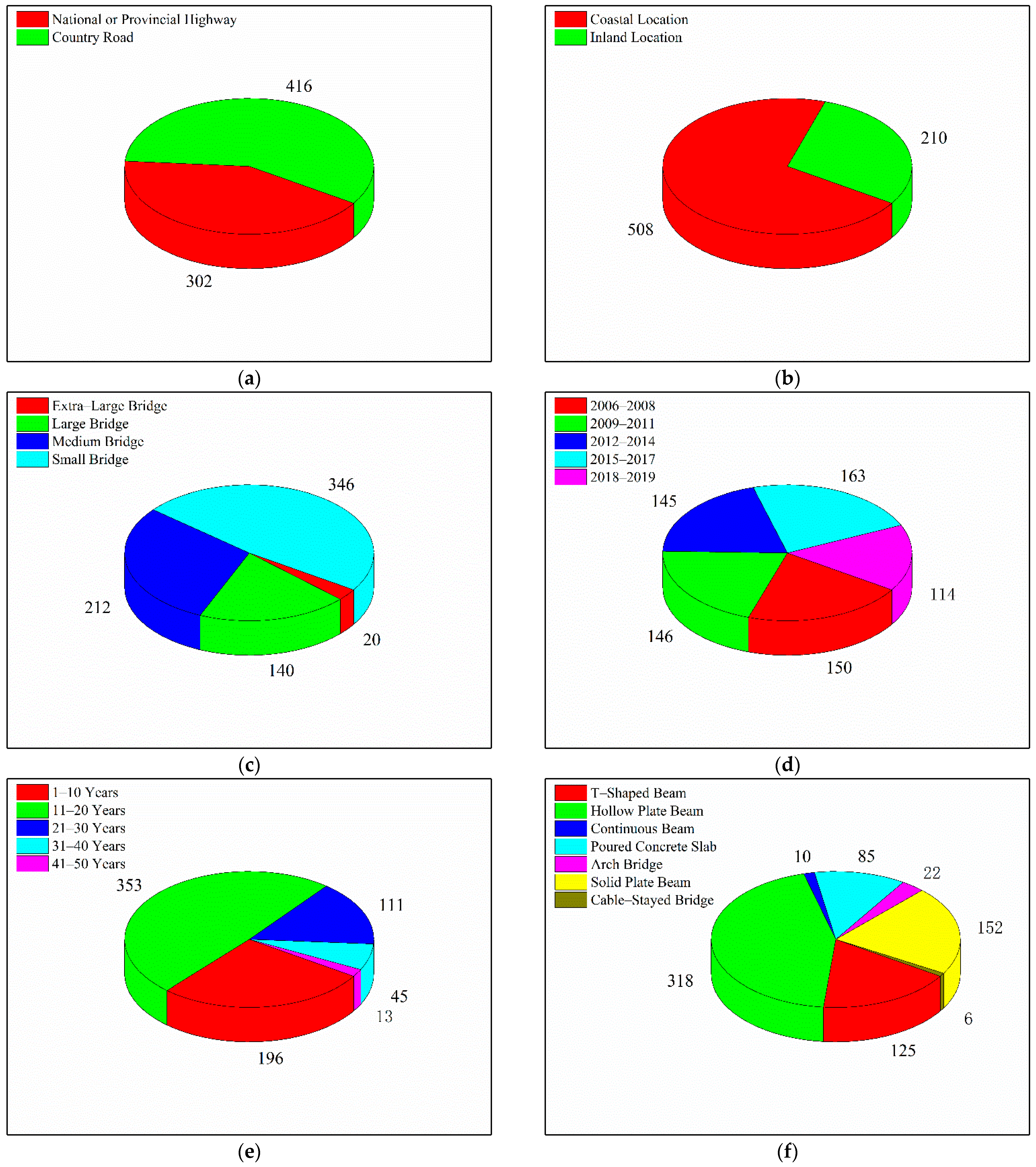
The cost associated with detecting bridge defects in coastal and inland areas of China, as determined by this study, is highly discrete and affected by a variety of factors. The data obtained is classified according to the six main factors (highway grade, bridge location, bridge grade, superstructure, bridge age, and detection time) that affect the cost of defect detection. The sample classification is presented in Figure 1; the total number of samples is 718.
In China, the cost of detecting bridge defects is regarded as a public financial expenditure. Government investment at all levels is affected by economic development [27]. Economic growth provides sufficient financial revenue for governments at all levels to manage bridges [28].
The GDP growth rate has been introduced as the seventh influencing factor to evaluate the comprehensive impact of socio-economic development on the investment in bridge defect detection. The past value of the GDP growth rate can be obtained on the government website, and its predicted value can also be obtained conveniently through existing forecasting models derived from economists. It has been widely used in operating cost prediction models [29,30]. The values are presented in Table 1. The classification standards of bridge grades refer to the Chinese standard “General Specifications for Design of Highway Bridges and Culverts”, and the details are presented in Table 2 [31].
3. Machine Learning-Based Bridge Defect Detection Cost Prediction Framework
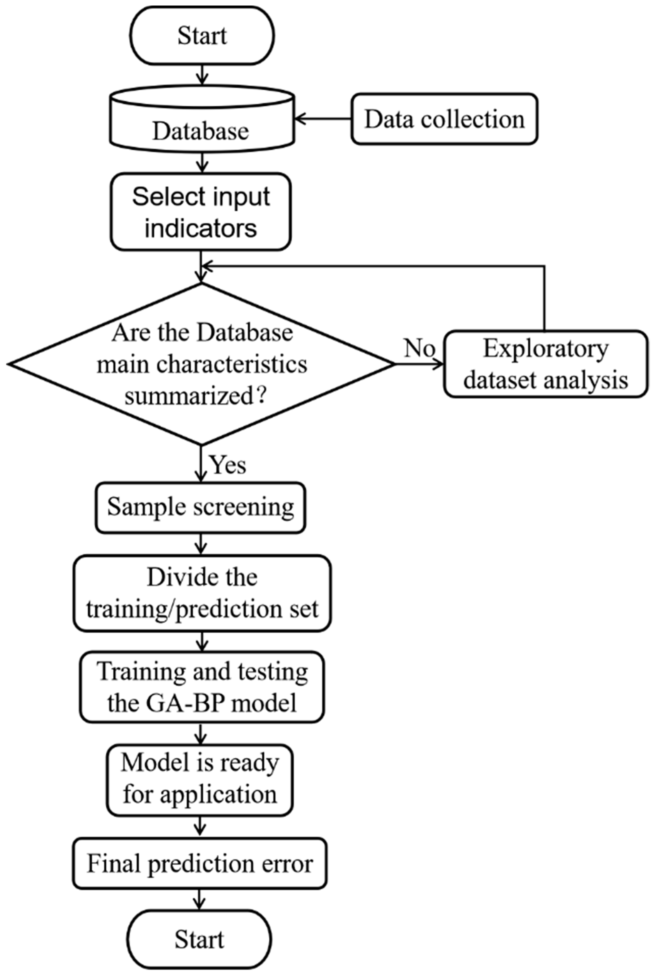
The recent and readily available advancements in computational power and data generation and storage capacities have been key in facilitating the use of machine learning approaches in different applications (e.g., classification, prediction, extraction, image and speech recognition, etc.). Therefore, this section introduces a machine learning-based framework for predicting the cost of bridge defect detection; the framework is presented in Figure 2. Before applying the machine learning methods, the raw bridge defect detection cost dataset was converted to a form most suitable for modeling. This included input indicators selection, exploratory data analysis, and sample screening. After the initial processing, the full dataset was split into a training set for developing machine learning models and a testing set for validating the prediction performances of the models.
3.1. Selection of Input Indicators Based on Random Forest
To improve the accuracy and operating efficiency of the prediction model, it was necessary to evaluate the degree of influence of various influencing factors on the defect detection cost and then select the indicators that have a significant impact on the defect detection cost. Random forest in machine learning was used to analyze the importance of factors in this study.
In machine learning, random forest is an ensemble learning method that contains multiple decision trees. It generates multiple classifiers (decision trees) at random and learns independently and makes predictions. The random forest approach has fast training speed, strong generalization, and anti-interference ability. It has wide applications and good results in the selection of indicators for highly discrete data and missing data [32,33]. The importance of a particular indicator was expressed by its variable importance measure (VIM) value [34].
We considered n indicators, X1, X2, X3…Xn. The training samples were extracted randomly to build decision trees. The prediction error rate for the remaining data in the sample database was calculated after sampling; these remaining samples are referred to as out-of-bag (OOB) data [35]. The observed value of variable Xj was then replaced at random and the tree was constructed again, and the prediction error rate of the OOB data was recalculated. Finally, the difference between the error rate of the two OOB data before and after the replacement was calculated. The average value for all trees after normalization gives the VIM () of variable Xj.
For variable Xj in the i-th tree, is
where is the number of observed OOB data of the i-th tree, is an indicator function that is 1 when the two values are equal and 0 when they are not equal, is the true result of the p-th observation, is the prediction result of the i-th tree for the p-th observation of OOB data before random replacement, and is the prediction result of the i-th tree for the p-th observation of OOB data after random replacement. When the variable j does not appear in the i-th tree, .
The VIM of variable Xj in the random forest is defined as
where n is the number of decision trees in the random forest.
3.2. Exploratory Data Analysis
To visually show the relationship between the selected data features and their labels in Section 3.1, an exploratory analysis of the bridge defect detection cost data is further carried out. Exploratory data analysis (EDA) is the process of evaluating the relationships among the different data features, assessing the relationship between the data features and labels, and selecting the main feature contributing to the considered labels [36]. Although results produced by either EDA or statistical analysis are used interchangeably, EDA is not identical to statistical analysis [37]. For example, statistical analysis depends on a priori that may or may not yield valid conclusions. However, EDA applies essentially no assumptions to the data in an effort to show its natural distribution [38].
3.3. Sample Screening
The practical engineering samples in the database are highly discrete. Each bridge for which detection work was conducted is unique. The samples have both statistical regularity and some outliers that are far away from similar samples. The occurrence of outliers does not indicate erroneous data, and the deletion of outliers would reduce the capacity of the sample database. To improve the prediction accuracy of the model without reducing the capacity of the sample database, the sample values were screened based on Bayes’ modified confidence test.
The samples were classified according to the indicators selected in the previous subsection. These samples Xi,j can be represented as at some arbitrary detection time tj. The algorithm for determining outliers in the sequence is as follows:
- (1)
- Let , where is the a priori uniform distribution according to the average characteristic parameter of degradation measure ;
- (2)
- Calculate the joint probability distribution of and as
- (3)
- Calculate the density function of the posterior distribution of as
- (4)
- Calculate the posterior expectation estimate as
- (5)
- Calculate the confidence interval of the degenerate section data based on the posterior expectation estimation method as
- (6)
- Calculate the confidence interval 1-α of the detected sample degradation measure at time t0 as
The comparatively high level of discreteness of the engineering samples was considered. In this study, we set α = 0.005. If ; then, it can be statistically determined that is an outlier.
3.4. GA-BP Model
Bridge defect detection cost is affected by many factors, and its prediction is a highly nonlinear regression problem. In view of the high nonlinearity, concurrent operation, self-adapting, and strong self-learning capability of the intelligent algorithm [39]. BP neural network model is proposed to predict the bridge defect detection cost and to solve the problems of current bridge detection cost assessment.
However, there are also some problems in the BP neural network model, for example, the uneasily determinable initial weights and easily local optimum [2]. The BP neural network model optimized by the application of GA global optimum characteristics can obtain the optimum initial weights quickly.
GA is a global optimization algorithm for simulating the biological evolution mechanism, which has been successfully integrated with BP neural network [40]. In recent years, GA-BP has been widely used in bridge reliability prediction, strength prediction of main girder concrete, and traffic volume prediction on bridges, and has achieved good results [41,42,43,44]. Therefore, this research used a machine learning method based on GA-BP to establish an intelligent prediction model. The genetic algorithm and BP neural network were combined to complement each other in predicting the cost of bridge detection.
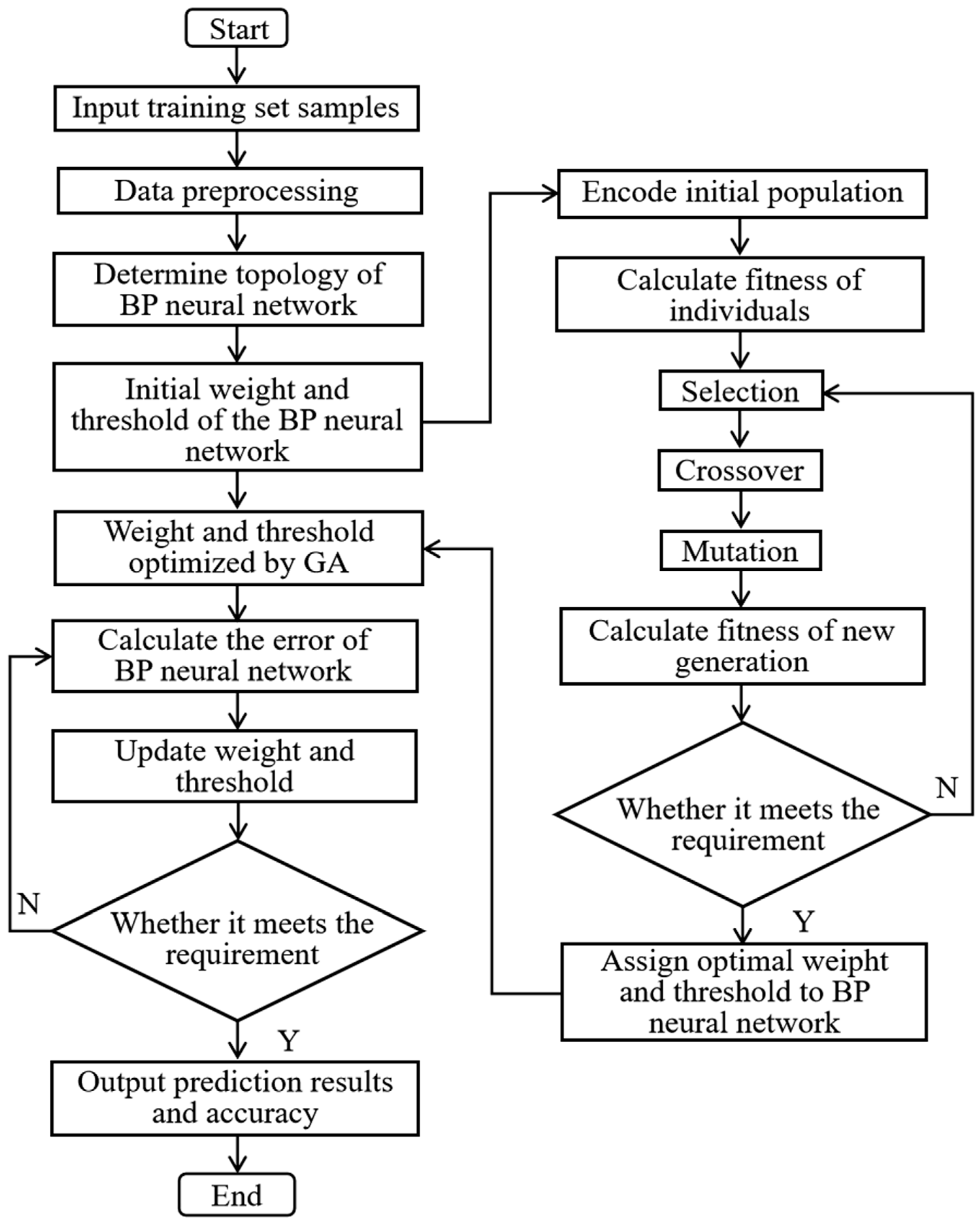
The principle of the GA-BP prediction model is as follows: the population in the GA is composed of multiple individuals, each of which is a character string composed of initial weights and thresholds of the BP neural network. The absolute value of the error between the predicted output, and the expected output is used as the fitness function to determine the advantages and disadvantages of each individual. The better individuals have a greater probability of being passed on to the next generation, and operations such as individual crossover and individual variation are applied to generate a new generation of populations and individuals [45]. After satisfying the GA termination condition, the initial weights and thresholds represented by the optimal individuals are assigned to the BP neural network [46].
The flowchart of the GA-BP prediction method is shown in Figure 3.
The specific implementation process of genetic algorithm to optimize BP neural network weights and thresholds is as follows:
- (1)
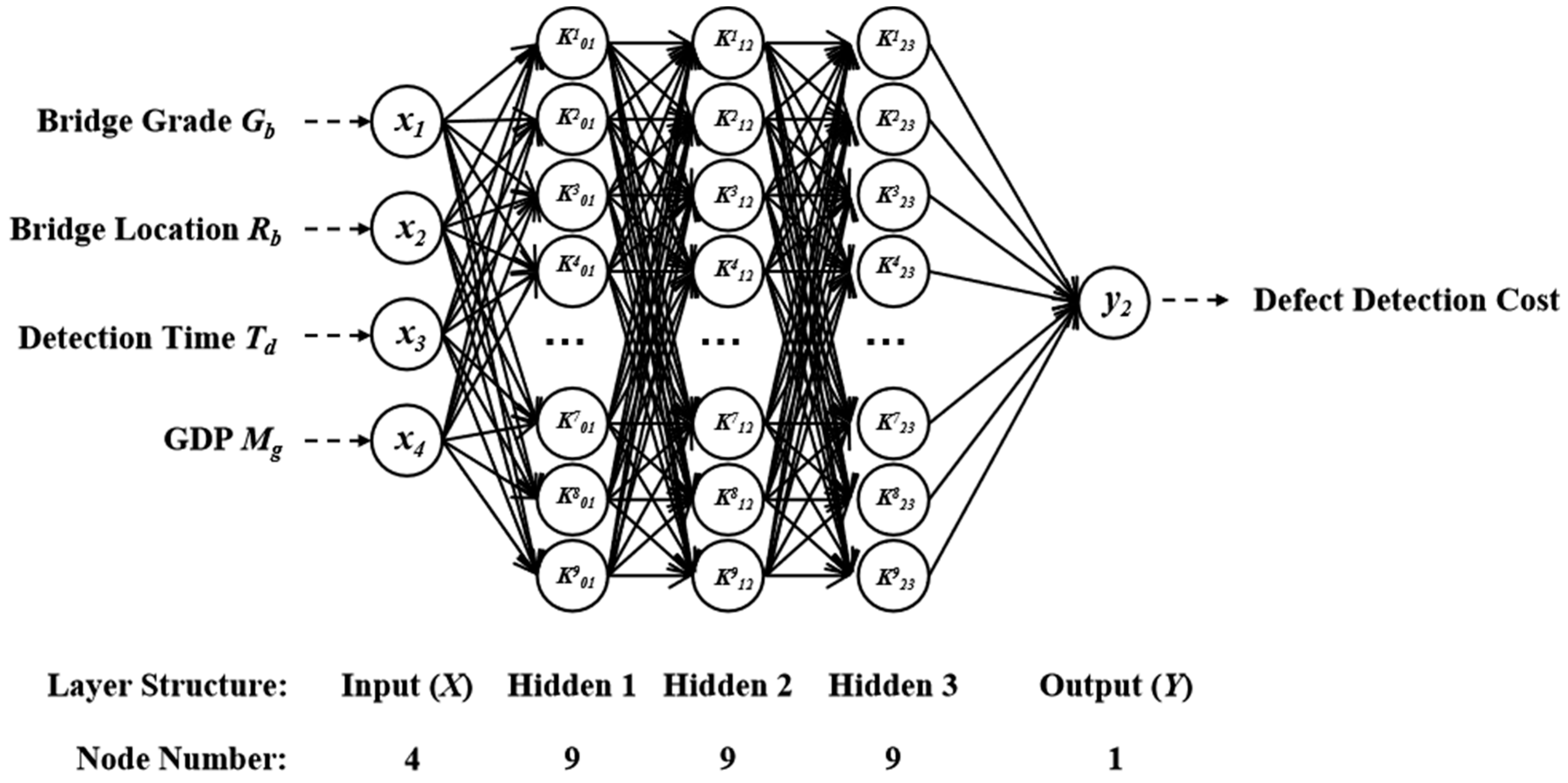
- Real coding is performed on the initial population, and the coding length can be calculated aswhere m1, m2, m3 are the number of nodes in each hidden layer; n is the number of input layer nodes; l is the number of output layer nodes.The neural network in this study contained five layers: one input layer, one output layer, and three fully connected hidden layers. Among them, the input layer contained four nodes, the output layer contained one node, and the hidden layers contained nine points per layer. The individual code length in this study was S = 4 × 9 + 9 × 9 + 9 × 9 + 9 × 1 = 207.The population size has a great influence on the global search performance of the genetic algorithm, which should be selected according to a specific problem [47]. The initial population size of this study was 30.
- (2)
- According to the individual coding value, the connection weights and thresholds between the layers of the BP neural network are obtained. The reciprocal of the sum of the absolute values of the prediction errors of the training data is used as the individual fitness value f. The calculation formula iswhere n is the number of samples; yi is the expected output of the i-th sample of BP neural network; zi is the predicted output of the i-th sample of BP neural network.
- (3)
- The roulette method is used to perform the genetic algorithm individual selection operation, that is, the selection strategy based on the fitness proportion. The selection probability pi of each individual i iswhere fi is the fitness value of individual i; k is the number of individuals in the population.
- (4)
- With the crossover probability Pc, the new individuals shall be generated by the crossover operation between the previous generation of individuals, and the individuals that do not experience the crossover operation shall be copied directly to the next generation. In this study, Pc = 0.4.
- (5)
- With the mutation probability Pm, the new individuals shall be generated, and the individuals that do not experience the mutation operation shall be copied directly to the next generation. In this study, Pm = 0.1.
- (6)
- Steps (2) to (5) are repeated until the number of training target iterations reaches the set target. The number of iterations in this study was 100.
The optimal individual in the population was selected for decoding after the iteration. The obtained initial weights and thresholds were used for training BP neural network model; thus, a bridge detection cost prediction model was established.
4. Machine Learning Implementation Results
4.1. Influencing Factors of Defect Detection Cost
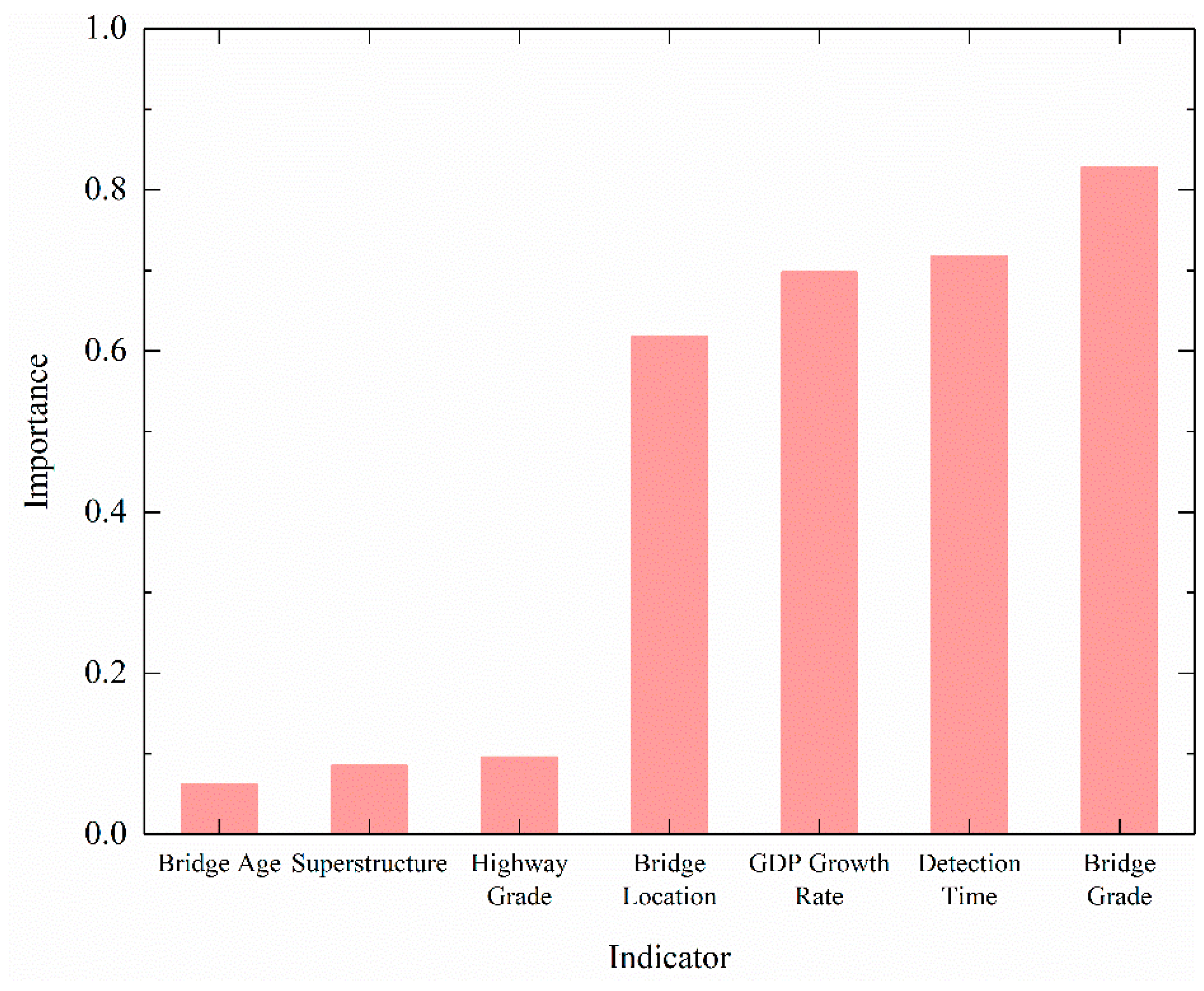
Based on the random forest algorithm mentioned in Section 3.1, the VIM of influencing factors (highway grade, bridge location, bridge grade, superstructure, bridge age, detection time, and GDP growth rate) was calculated. The calculation results are shown in Figure 4.
It can be seen from Figure 4 that four indicators (bridge grade, detection time, GDP growth rate, and bridge location) have importance values greater than 0.6. These four indicators are significantly more important than the remaining indicators of highway grade, superstructure, and bridge age, which have importance values of less than 0.1. Thus, the bridge grade, detection time, bridge location, and GDP growth rate were selected as the input indicators for the proposed prediction model.
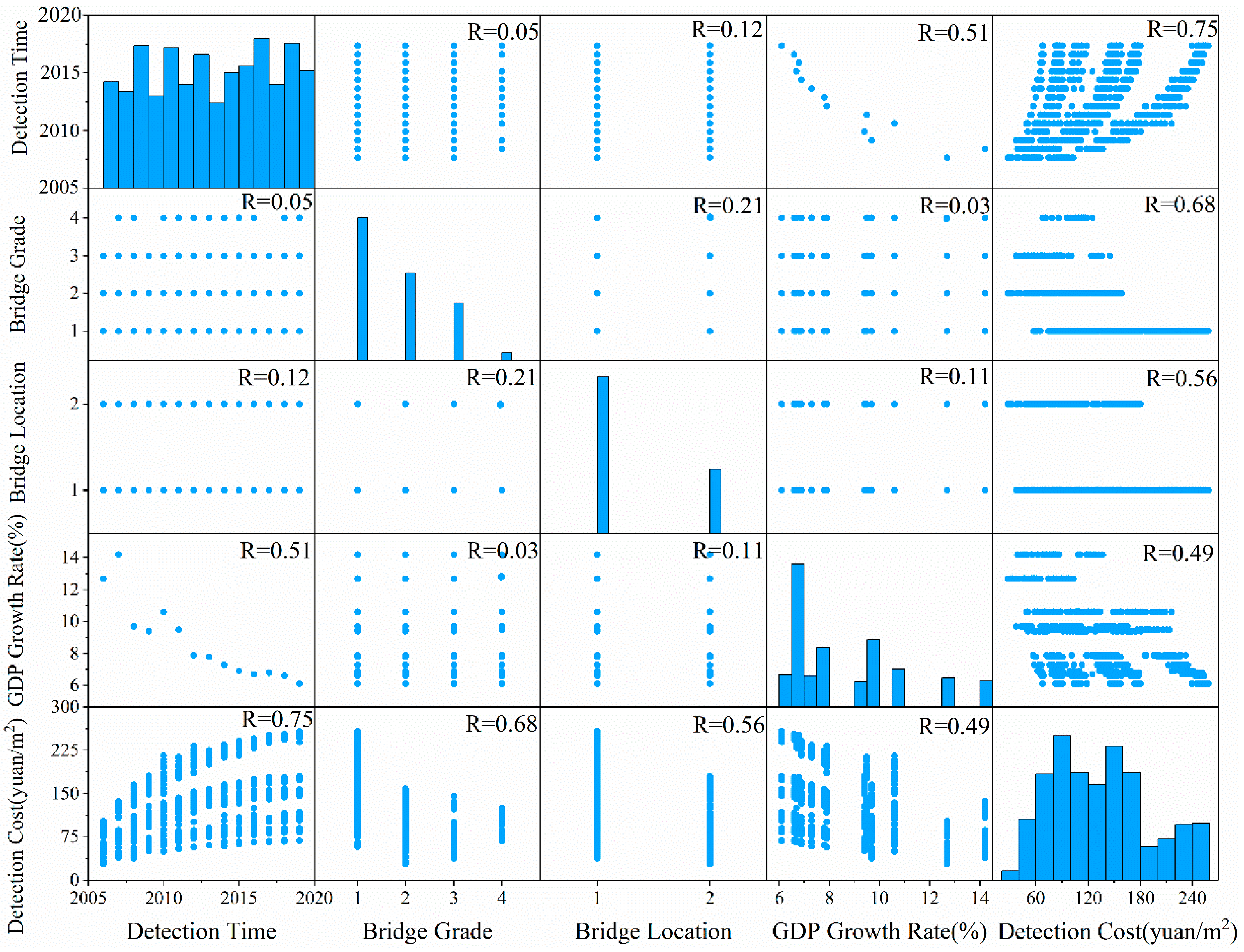
To verify the correlation between the four input indicators and the bridge defect detection cost, and visually show the relationship between different input parameters and detection cost, the EDA scatterplot matrix was used for exploratory data analysis of the database. The scatterplot matrix presents two types of two-dimensional subplots. Each off-diagonal subplot represents the relationship (scatter) between the features on the intersecting row and column. The diagonal subplots on the other hand are histograms, with each having a vertical axis that represents the frequency associated with the specific feature given on the horizontal axis. Therefore, the scatterplot matrix, shown in Figure 5, consisted of 25 subplots (5 by 5 matrix) divided into 20 scatter and 5 frequency plots. As can be seen in Figure 5, although no well-identified fit can describe the data per se, the correlation between different detection cost features can still be inferred.
4.2. Sample Classification Based on Selected Indicators
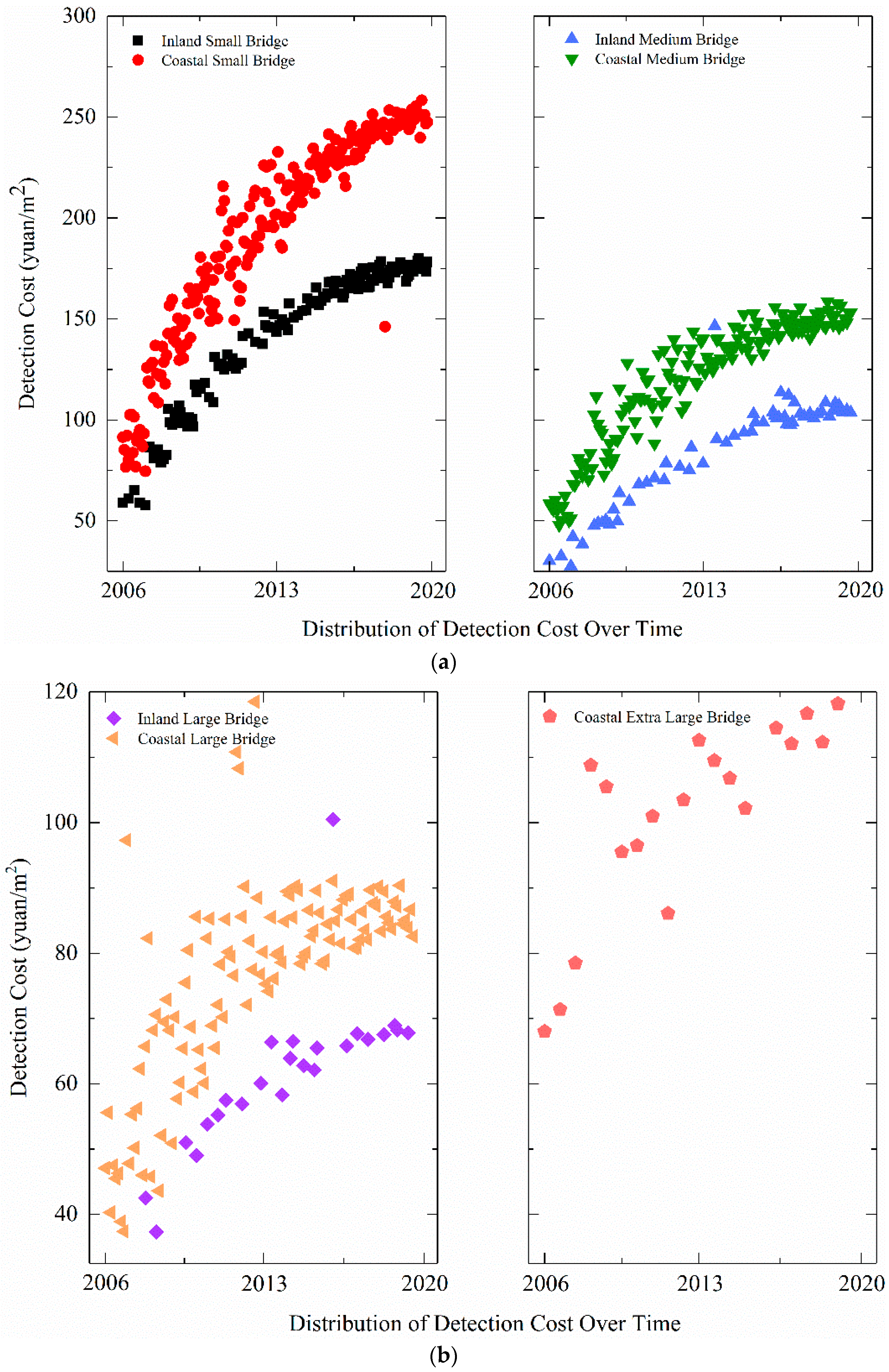
The classification of all samples based on the selected indicators is shown in Figure 6. Considering a one-to-one correspondence between the GDP growth rate and the detection time, the figure only includes three indicators: bridge grade, bridge location, and detection time.
It can be seen from Figure 6 that the detection cost samples were divided into four categories according to the bridge grade: small bridge, medium bridge, large bridge, and extra-large bridge. Each category was then divided into two sub-categories according to the location (coastal or inland) of the bridge. Finally, the samples were sorted according to detection time. The sample values tend to decrease first and then increase as the bridge grade increases. The sample values of coastal areas in the same period are higher than those of inland areas, and the gap tends to expand with time. The sample values have a relatively obvious correlation with time, which shows that the method of predicting future detection costs based on the above classification is feasible.
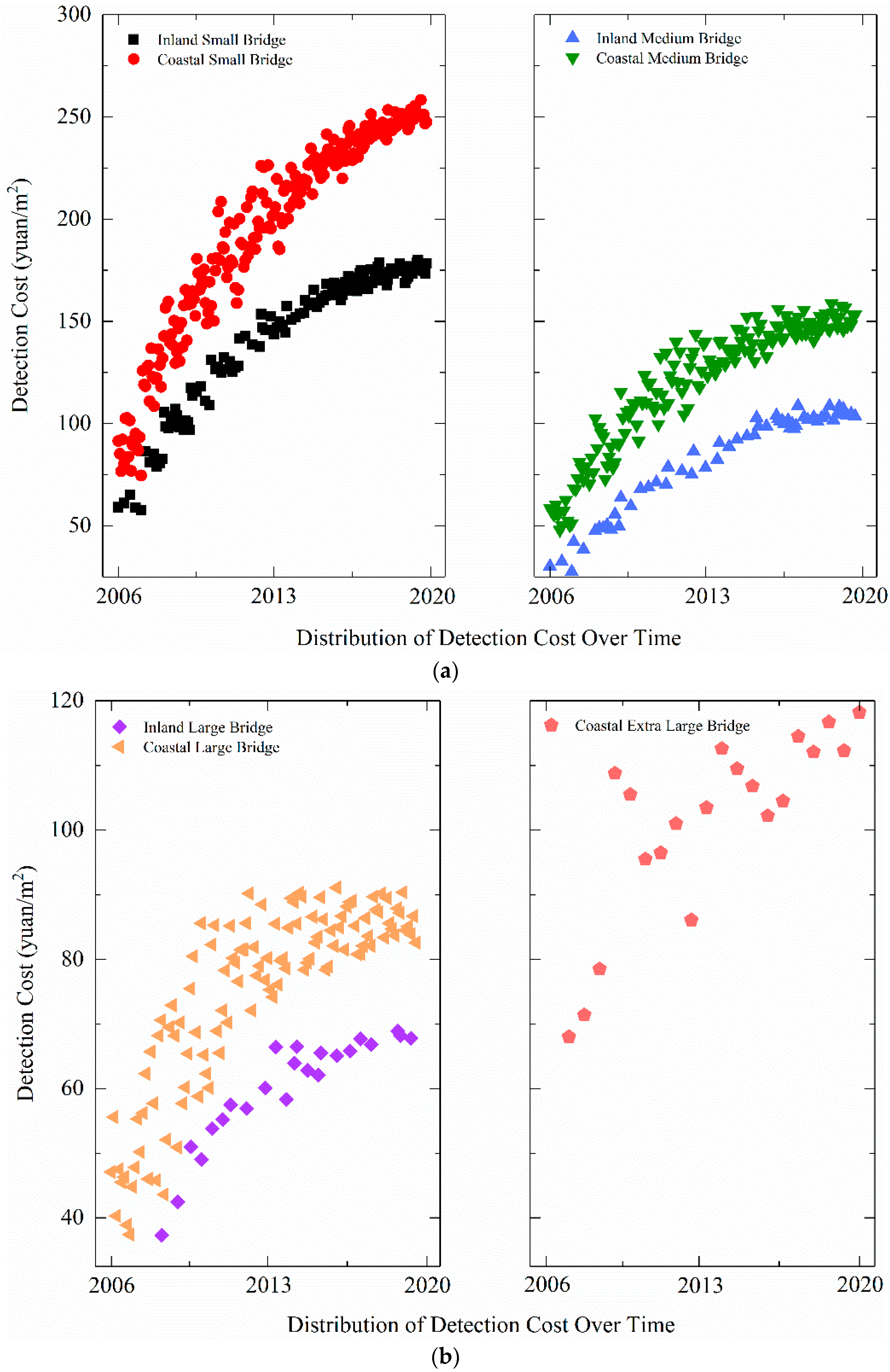
Therefore, as not to decrease the sample size, the outliers were replaced by the average of the corresponding data series after their identification. A total of 19 detection samples (2.6% of the total) were identified as outliers and replaced after data screening. The sample distribution after the replacement is shown in Figure 7.
4.3. Structure of Sample Database
All 718 detection cost samples were selected for training. The samples were classified according to the bridge location and bridge grade and then were sequenced according to the detection time. Then, 80% of samples with the earliest detection times in each type of data were placed into the training set, and 20% of samples with the latest detection times formed the prediction set. For the period 2016–2018, the starting time of the predictions for different data types was different. There were 575 samples in the training set and 143 samples in the prediction set. The detailed division of the sample size is plotted in Table 3.
4.4. Topology of GA-BP Model
Each sample was stored as a 1 × 5 matrix, where the first four columns represent the bridge location, bridge grade, detection time, and GDP growth rate, and the fifth column denotes the detection cost. The 575 training set samples formed a 575 × 5 matrix, and the 143 prediction set samples formed a 143 × 5 matrix. These were substituted into the GA-BP model for analysis.
The topology of the detection cost prediction model is shown in Figure 8.
4.5. Prediction Software for Bridge Defect Detection Cost
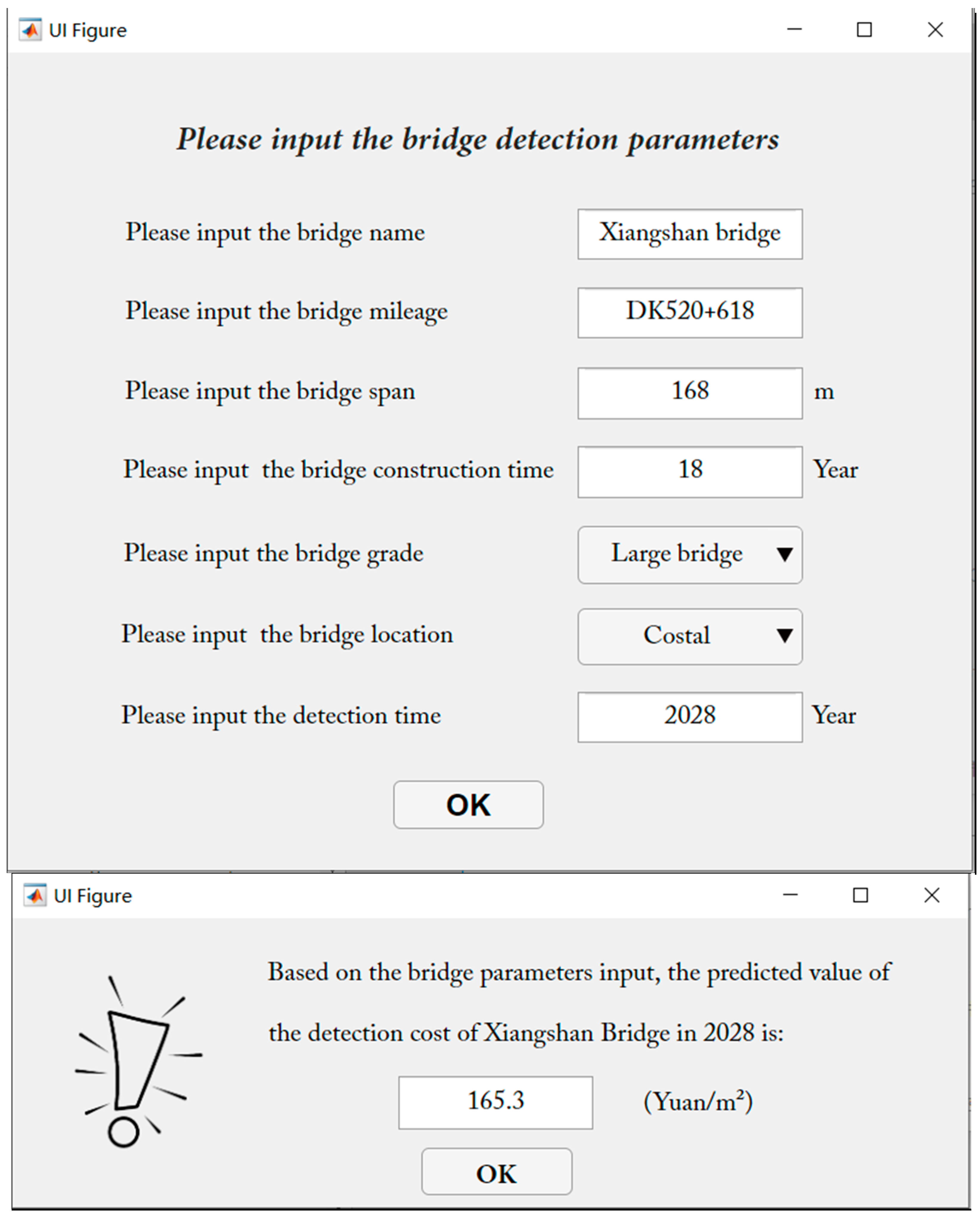
With the GA-BP prediction model as its core, a “Prediction software for Bridge Detection Cost” was established using the MATLAB platform. The open database format was used to merge future detection cost information into the database. Sample information can be updated or changed in the database, and basic information such as the bridge name and bridge span can be input via the software interface. The bridge grade and location are selected through a drop-down menu, and the year for which the detection cost needs to be predicted can be input. The software was established with the help of a coursebook written by Hahn et al. [48]. The software interface is shown in Figure 9.
In this study, the prediction model established by Jiang et al. [49] for the Chinese GDP growth rate was adopted and built into the software developed. Other economic indicators besides the GDP growth rate can be adopted to consider the impact of time-dependent social and economic developments on the software.
4.6. Accuracy Analysis of Software Prediction
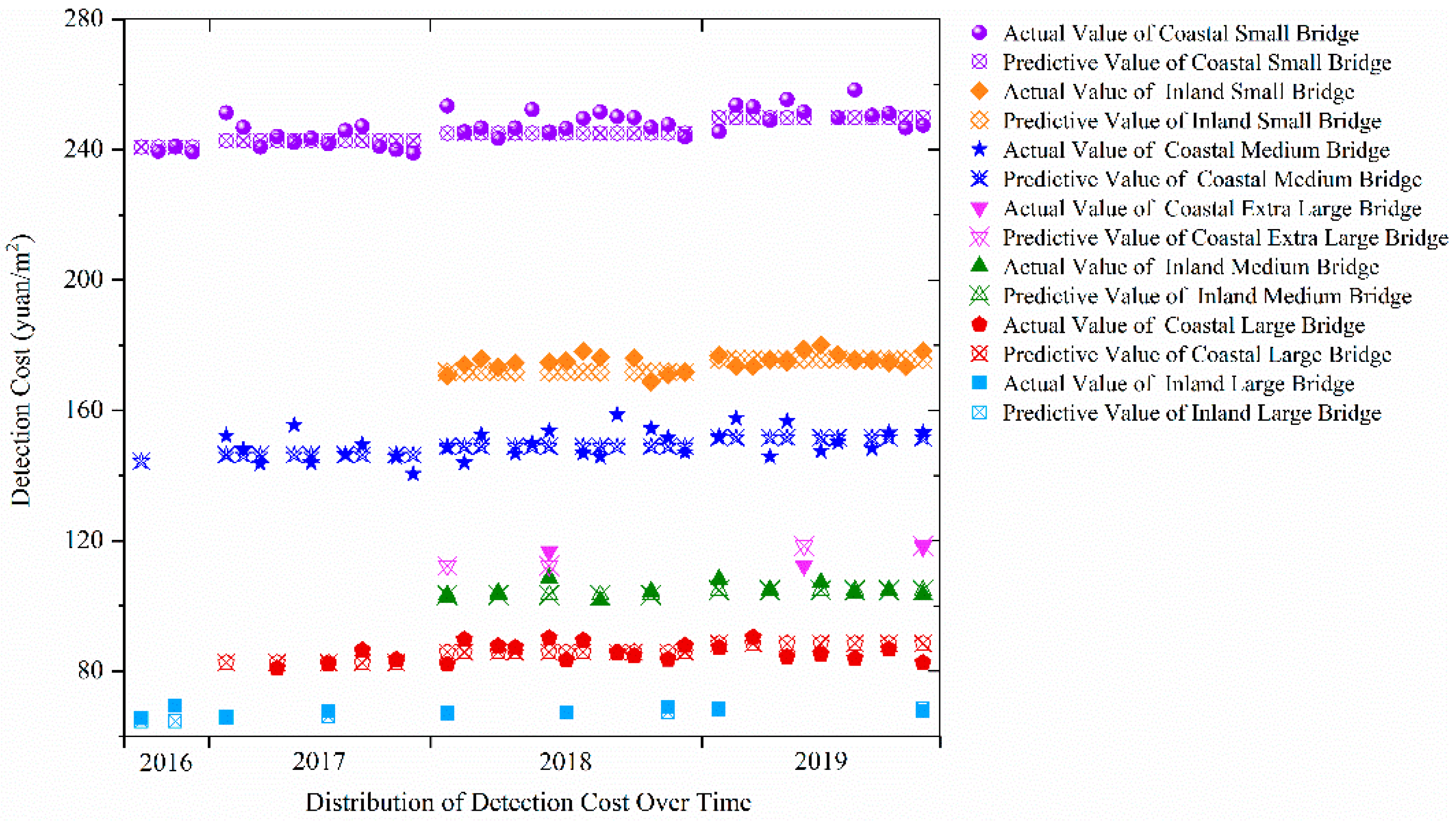
The software obtained through the above training procedure was used to predict the samples in the prediction set, and the results were compared with the practical bridge detection costs. The coefficient of determination of the training set is 0.985, and the coefficient of determination of the prediction set is 0.973. A comparison of the predicted values and the actual values under the corresponding indicators is shown in Figure 10. The values shown in the figure are for the test dataset only. It can be seen that the prediction model effectively estimates the changes in detection costs in the prediction set through training and learning from historical data.
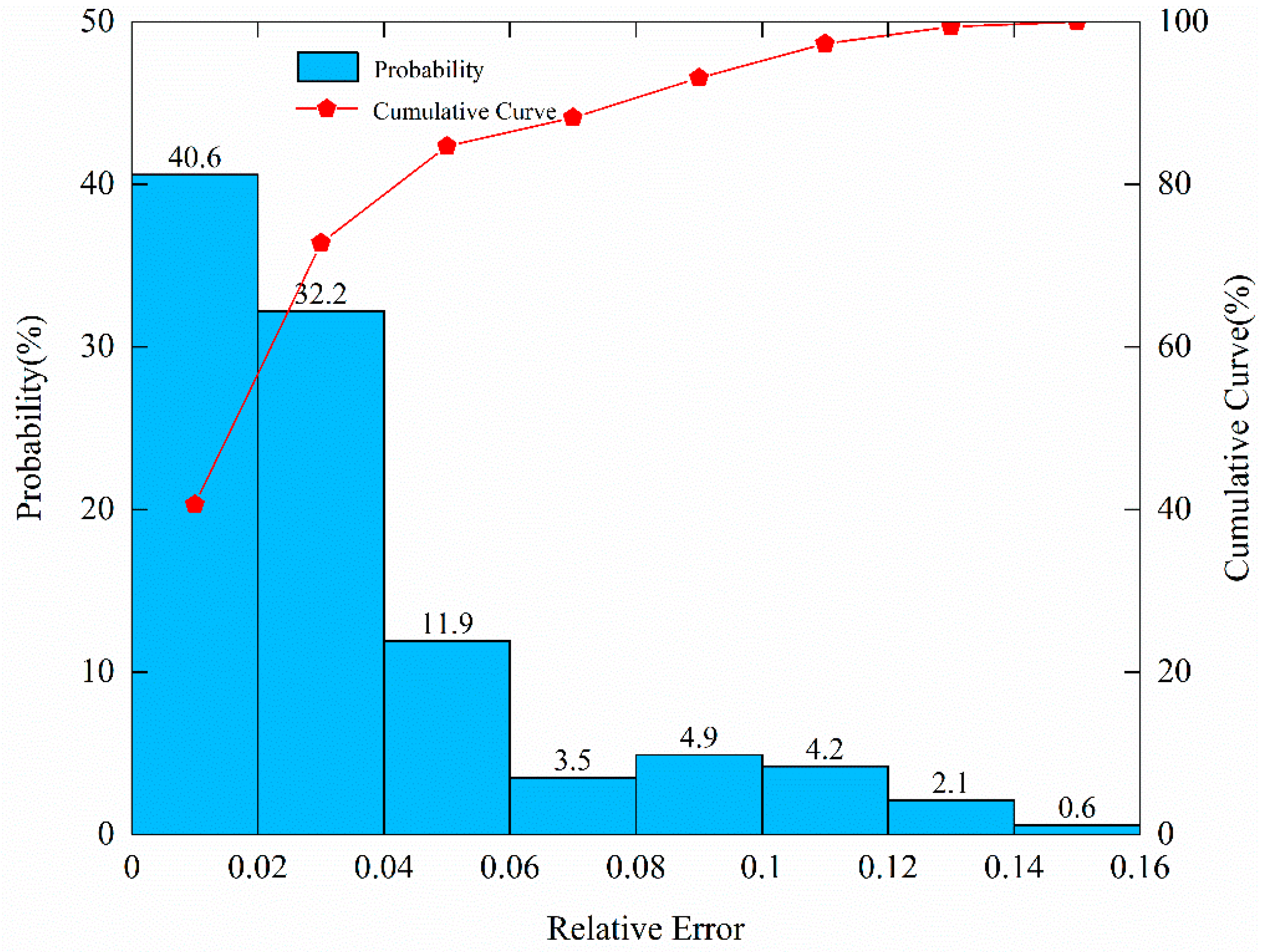
The relevant prediction error indicators are presented in Table 4, and the distribution of the relative error is shown in Figure 11. Table 4 indicates that the average error is 4.6 Yuan/m2, with a maximum error of 13.3 Yuan/m2 and a minimum error of 0 Yuan/m2. The average relative error is 3.41%, the maximum is 14.76%, and the minimum is 0%. It can be seen from Figure 11 that, for 83% of the prediction data, the relative error is less than 5%. For 93% of the prediction data, the relative error is less than 10%. The predicted values given by the model agree well with the practical values.
5. Conclusions
This paper has described the construction of a defect detection cost sample database based on practical engineering data from 386 bridges in coastal and inland areas of China from 2006 to 2019. A bridge defect detection cost prediction model and the relevant software were also developed based on a machine learning approach. With the prediction model as the core, an intelligent prediction software for the cost of detecting bridge defects was established for engineering applications. Based on the results of this study, the following conclusions can be drawn:
- (1)
- The random forest method was adopted to evaluate the importance of the seven main factors affecting the detection cost. The results show that the measures of the importance of four indicators of bridge grade, detection time, GDP growth rate, and bridge location are all greater than 0.6, which is significantly higher than the remaining indicators of highway grade, superstructure, and bridge age, whose measures of importance are all less than 0.1.
- (2)
- Bayes’ modified confidence test was adopted to the outliers in the detection data that have a relatively large disparity with respect to the detection costs of similar bridges, and which may affect the prediction accuracy. The results show that 19 detection samples, constituting 2.6% of the total number of samples, were identified as outliers. These were replaced by the average value of similar data.
- (3)
- The GDP growth rate of China over recent years was adopted to consider the impact of social and economic developments on the detection costs. The prediction model was then established based on a genetic algorithm combined with a neural network. A comparison of the predicted and practical values indicates that the average model error is 4.6 Yuan/m2 and the average relative error is 3.41%. For 83% of the prediction data, the relative error is less than 5%; for 93% of the prediction data, the relative error is less than 10%.
- (4)
- With the prediction model as the core, an intelligent prediction software for the cost of bridge detection was established for engineering applications based on the MATLAB software platform. It can provide data reference for evaluating management costs and calculating life-cycle costs in bridges.
6. Prospect
There are several limitations in this paper, which can inform the direction of future studies. The sample size of the database was limited, and the coverage was not wide enough. As a result, indicators such as geological conditions and extreme weather conditions were not fully considered. A more comprehensive bridge defect detection cost database is needed to support future studies. Additionally, the cost of defect detection is also related to the detection technique and management mode. When they change significantly, the previously trained model will no longer be applicable. The samples should be collected anew for training. Finally, the input indicators selected in this paper may not accurately reflect the degree of influence of various factors affecting bridge defect detection costs due to insufficient sample size. Future studies should extensively collect more samples and divide the samples in more detail according to the external environment and bridge types to improve the prediction accuracy and application scope.
The results presented in this study demonstrate that the software developed in this paper can be applied successfully to predict the bridge defect detection cost. The developed software is simple to operate and easy to use, which can be used for rapid assessment of bridge life-cycle defect detection cost. Additionally, the software can help bridge management departments to formulate more economical bridge defect detection programs and can also be used to prepare bridge operating investment budgets. Countries or regions outside of China should use the local bridge defect detection cost database when using the software. Similarly, economic development indicators should also use the local GDP growth rate or other economic development indicators. Moreover, it is necessary to rescreen the input indicators of the model and software and use the exhaustive method based on grid search to reset the relevant parameters of the neural network, such as the number of network layers, the number of neurons in each layer, etc.
Author Contributions
Writing original draft preparation, C.W.; data curation, C.Y.; software, S.Z.; writing review and editing, Y.L. and B.Q. All authors have read and agreed to the published version of the manuscript.
Funding
This research was funded by [China Railway Major Bridge Reconnaissance and Design Institute Co., Ltd] grant number [2016YFC0802202-2].
Data Availability Statement
Some or all data, models, or code that support the findings of this study are available from the corresponding author upon reasonable request.
Acknowledgments
The writers acknowledge the partial financial support of the China Railway Major Bridge Reconnaissance and Design Institute Co., Ltd. through 2016YFC0802202-2. The writers thank the Foshan Transportation Bureau, the Deyang Transportation Bureau, the Sichuan Communication Surveying and Design Institute, and other departments that are unwilling to disclose their names for providing valuable original data support. Many additional Sichuan Communication Surveying and Design Institute personnel provided suggestions and insights. Their contributions positively influenced this research effort.
Conflicts of Interest
The authors declare no conflict of interest. The contents of this paper reflect the views of the writers and not necessarily the views of Southwest Jiaotong University. The writers are responsible for the facts and the accuracy of the data presented in this paper. The contents do not necessarily reflect the official views or policies of either the Foshan Transportation Bureau or the Deyang Transportation Bureau at the time of publication.
References
- Ghodoosi, F.; Bagchi, A.; Zayed, T. Reliability-based condition assessment of an externally restrained bridge deck system considering uncertainties in key design parameters. J. Perform. Constr. Facil. 2016, 30, 04014189. [Google Scholar] [CrossRef]
- Shim, H.S.; Lee, S.H. Developing a probable cost analysis model for comparing bridge deck rehabilitation methods. KSCE J. Civil Eng. 2016, 20, 68–76. [Google Scholar] [CrossRef]
- Eamon, C.D.; Jensen, E.A.; Grace, N.F.; Shi, X. Life-Cycle Cost Analysis of alternative reinforcement materials for bridge superstructures considering cost and maintenance uncertainties. J. Mater. Civ. Eng. 2012, 24, 373–380. [Google Scholar] [CrossRef] [Green Version]
- Shivang, S.; Ghosh, J. A metamodeling based seismic life-cycle cost assessment framework for high-way bridge structures. Reliab. Eng. Syst. Saf. 2020, 195, 106724. [Google Scholar]
- Kong, J.S.; Frangopol, D.M. Life-cycle reliability-based maintenance cost optimization of deteriorating structures with emphasis on bridges. J. Struct. Eng. 2003, 129, 818–828. [Google Scholar] [CrossRef]
- Thompson, P.D.; Small, E.P.; Johnson, M.; Marshall, A.R. The Pontis Bridge Management System. Struct. Eng. Int. 1998, 8, 303–308. [Google Scholar] [CrossRef]
- Lee, J.H.; Choi, Y.; Ann, H.; Jin, S.Y.; Lee, S.-J.; Kong, J.S. maintenance cost estimation in psci girder bridges using updating probabilistic deterioration model. Sustainability 2019, 11, 6593. [Google Scholar] [CrossRef] [Green Version]
- Echaveguren, T.; De Concepción, U.; Dechent, P. Allocation of bridge maintenance costs based on prioritization indexes. Rev. Construcción 2019, 18, 568–578. [Google Scholar] [CrossRef]
- Shi, X.; Zhao, B.; Yao, Y.; Wang, F. Prediction methods for routine maintenance costs of a reinforced concrete beam bridge based on panel data. Adv. Civ. Eng. 2019, 2019, 5409802. [Google Scholar] [CrossRef] [Green Version]
- Ghodoosi, F.; Abu-Samra, S.; Zeynalian, M.; Zayed, T. Maintenance Cost Optimization for Bridge Structures Using System Reliability Analysis and Genetic Algorithms. J. Constr. Eng. Manag. 2018, 144, 04017116. [Google Scholar] [CrossRef]
- Huang, Y.-H.; Huang, H.-Y. A model for concurrent maintenance of bridge elements. Autom. Constr. 2012, 21, 74–80. [Google Scholar] [CrossRef]
- Montazeri, N.; Touran, A. Applied Decision-Making Framework for Maintenance Scheduling in Bridge Management. In Proceedings of the Creative Construction Conference 2019, Budapest, Hungary, 29 June–2 July 2019; Periodica Polytechnica Budapest University of Technology and Economics: Budapest, Hungary, 2019. [Google Scholar]
- Gomes, W.J.; Beck, A.T.; Haukaas, T. Optimal inspection planning for onshore pipelines subject to external corrosion. Reliab. Eng. Syst. Saf. 2013, 118, 18–27. [Google Scholar] [CrossRef]
- Huang, H.; Burton, H.V. Classification of in-plane failure modes for reinforced concrete frames with infills using machine learning. J. Build. Eng. 2019, 25, 100767. [Google Scholar] [CrossRef]
- Sediek, O.A.; El-Tawil, S.; McCormick, J. Seismic debris field for collapsed RC moment resisting frame buildings. J. Struct. Eng. 2021, 147, 04021045. [Google Scholar] [CrossRef]
- Zhang, Y.; Burton, H.V.; Sun, H.; Shokrabadi, M. A machine learning framework for assessing post-earthquake structural safety. Struct. Saf. 2018, 72, 1–16. [Google Scholar] [CrossRef]
- Siam, A.; Ezzeldin, M.; El-Dakhakhni, W. Machine learning algorithms for structural performance classifications and predictions: Application to reinforced masonry shear walls. In Structures; Elsevier: Amsterdam, The Netherlands, 2019; pp. 252–265. [Google Scholar]
- Neves, A.C.; González, I.; Leander, J.; Karoumi, R. A new approach to damage detection in bridges using machine learning. In Proceedings of the International Conference on Experimental Vibration Analysis for Civil Engineering Structure, Germany, San Diego USA, 12–14 July 2017; Springer Science and Business Media LLC: Berlin/Heidelberg, Germany. [Google Scholar]
- Mustapha, S.; Kassir, A.; Hassoun, K.; Dawy, Z.; Abi-Rached, H. Estimation of crowd flow and load on pedestrian bridges using machine learning with sensor fusion. Autom. Constr. 2020, 112, 103092. [Google Scholar] [CrossRef]
- Assaad, R.; El-Adaway, I. Bridge Infrastructure Asset Management System: Comparative Computational Machine Learning Approach for Evaluating and Predicting Deck Deterioration Conditions. J. Infrastruct. Syst. 2020, 26, 04020032. [Google Scholar] [CrossRef]
- Yang, D.Y.; Frangopol, D.M. Life-cycle management of deteriorating bridge networks with net-work-level risk bounds and system reliability analysis. Struct. Saf. 2020, 83, 101–111. [Google Scholar] [CrossRef]
- Lim, S.; Chi, S. Xgboost application on bridge management systems for proactive damage estimation. Adv. Eng. Inform. 2019, 41, 108–122. [Google Scholar] [CrossRef]
- Widodo, S.J.; Tri, J.W.A.; Anwar, N.; Hajek, P.; Han, A.L.; Kristiawan, S.; Chan, W.T.; Ismail, M.B.; Gan, B.S.; Sriravindrarajah, R. Dynamic bayesian updating approach for predicting bridge condition based on Indonesia-bridge management system (I-BMS). In Proceedings of the International Conference on Rehabilitation and Maintenance in Civil Engineering, EDP Sciences, Solo Baru, Solo, Indonesia, 11–12 July 2018. [Google Scholar]
- Nogueira, C.G.; Leonel, E.D. Probabilistic models applied to safety assessment of reinforced concrete structures subjected to chloride ingress. Eng. Fail. Anal. 2013, 31, 76–89. [Google Scholar] [CrossRef]
- Saad, L.; Aissani, A.; Chateauneuf, A.; Raphael, W. Reliability-based optimization of direct and indirect LCC of RC bridge elements under coupled fatigue-corrosion deterioration processes. Eng. Fail. Anal. 2016, 59, 570–587. [Google Scholar] [CrossRef]
- Kim, C.; Lee, E.-B.; Harvey, J.T.; Fong, A.; Lott, R. Automated sequence selection and cost calculation for maintenance and rehabilitation in highway Life-Cycle Cost Analysis (LCCA). Int. J. Transp. Sci. Technol. 2015, 4, 61–75. [Google Scholar] [CrossRef] [Green Version]
- Zhang, J.S.; Tan, W. Research on the Coupling Coordinative Degree of Transportation and Regional Economy in China. Adv. Mater. Res. 2011, 403–408, 1732–1735. [Google Scholar] [CrossRef]
- Chen, A.; Pan, Z.; Ma, R.; Wang, D. New development of mesoscopic research on durability performance of structural concrete in bridges. China J. Highw. Transp. 2016, 29, 42–48. [Google Scholar]
- Bastami, R.; Bazzazi, A.A.; Shoormasti, H.H.; Ahangari, K. Prediction of blasting cost in limestone mines using gene expression programming model and artificial neural networks. J. Min. Environ. 2020, 11, 281–300. [Google Scholar]
- Chi, S.; Bunker, J.; Teo, M. Measuring impacts and risks to the public of a privately operated toll road project by considering perspectives in cost-benefit analysis. J. Transp. Eng. Part A Syst. 2017, 143, 04017060. [Google Scholar] [CrossRef] [Green Version]
- China Communications Press Co., L. General Specifications for Design of Highway Bridges and Culverts; JTG D60-2015; Ministry of Transport of the People’s Republic of China: Beijing, China, 2015.
- Sun, D.; Wen, H.; Wang, D.; Xu, J. A random forest model of landslide susceptibility mapping based on hyperparameter optimization using Bayes algorithm. Geomorphology 2020, 362, 107201. [Google Scholar] [CrossRef]
- Tang, Z.; Mei, Z.; Liu, W.; Xia, Y. Identification of the key factors affecting Chinese carbon intensity and their historical trends using random forest algorithm. J. Geogr. Sci. 2020, 30, 743–756. [Google Scholar] [CrossRef]
- Richard, C.; Thomas, C.; Karen, H.E.B.; Adele, C. Random forests for classification in ecology. Ecology 2007, 88, 2783–2792. [Google Scholar]
- Breiman, L. Bagging Predictors. Mach. Learn. 1996, 24, 123–140. [Google Scholar] [CrossRef] [Green Version]
- Urminder, S.; Manhoi, H.; Karin, D.; Syrkin, W.E. MetaOmGraph: A workbench for interactive exploratory data analysis of large expression datasets. Nucleic Acids Res. 2020, 4, 4–16. [Google Scholar]
- Xiao, C.; Ye, J.; Esteves, R.M.; Rong, C. Using Spearman’s correlation coefficients for exploratory data analysis on big dataset. Concurr. Comput. Pract. Exp. 2016, 28, 3866–3878. [Google Scholar] [CrossRef]
- Velleman, P.F.; Hoaglin, D.C. Applications, Basics, and Computing of Exploratory Data Analysis; Duxbury Press: Pacific Grove, CA, USA, 1981. [Google Scholar]
- Chunyan, L.; Jianchun, L.; Linyuan, K. Performance comparison between GA-BP neural network and BP neural network. Chin. J. Health Stat. 2013, 30, 173–176. [Google Scholar]
- Wang, S.; Zhang, N.; Wu, L.; Wang, Y. Wind speed forecasting based on the hybrid ensemble empirical mode decomposition and GA-BP neural network method. Renew. Energy 2016, 94, 629–636. [Google Scholar] [CrossRef]
- Jianxi, Y.; Jianting, Z.; Fan, W. A study on the application of GA-BP neural network in the bridge reliability Assessment. In Proceedings of the 2008 International Conference on Computational Intelligence and Security, Suzhou, China, 13–17 December 2008. [Google Scholar]
- Shi, R.; Zhong, W.; Zhang, H.; Chen, H.; Ji, X. Predictions of concrete compressive strength based a hybrid algorithm of GA-BP. In Proceedings of the Proceedings of the 4th Annual International Conference on Material Engineering and Application (ICMEA 2017), Wuhan, China, 15–17 December 2017; Atlantis Press: Amsterdam, The Netherlands, 2018. [Google Scholar]
- Peng, Y.; Xiang, W. Short-term traffic volume prediction using GA-BP based on wavelet denoising and phase space reconstruction. Phys. A Stat. Mech. Appl. 2020, 549, 123913. [Google Scholar] [CrossRef]
- Zheng, D.; Qian, Z.-D.; Liu, Y.; Liu, C.-B. Prediction and sensitivity analysis of long-term skid resistance of epoxy asphalt mixture based on GA-BP neural network. Constr. Build. Mater. 2018, 158, 614–623. [Google Scholar] [CrossRef]
- Harpham, C.; Dawson, C.; Brown, M.R. A review of genetic algorithms applied to training radial basis function networks. Neural Comput. Appl. 2004, 13, 193–201. [Google Scholar] [CrossRef]
- Salajegheh, E.; Gholizadeh, S. Optimum design of structures by an improved genetic algorithm using neural networks. Adv. Eng. Softw. 2005, 36, 757–767. [Google Scholar] [CrossRef]
- Liang, Y.-J.; Ren, C.; Wang, H.-Y.; Huang, Y.-B.; Zheng, Z.-T. Research on soil moisture inversion method based on GA-BP neural network model. Int. J. Remote Sens. 2019, 40, 2087–2103. [Google Scholar] [CrossRef]
- Hahn, B.H.; Valentine, D.T. Essential MATLAB for Engineers and Scientists; Academic Press: Cambridge, MA, USA, 2016. [Google Scholar]
- Jiang, Y.; Guo, Y.; Zhang, Y. Forecasting China’s GDP growth using dynamic factors and mixed-frequency data. Econ. Model. 2017, 66, 132–138. [Google Scholar] [CrossRef]
Figure 1.
Bridge defect detection cost classification (a) highway grade (b) bridge location (c) bridge grade (d) detection time (e) bridgc age (f) superstructure.
Figure 1.
Bridge defect detection cost classification (a) highway grade (b) bridge location (c) bridge grade (d) detection time (e) bridgc age (f) superstructure.

Figure 2.
Machine learning implementation framework.

Figure 3.
Flowchart of GA-BP model.

Figure 4.
Calculation results for variable importance measures.

Figure 5.
Scatterplot matrix for selected input indicators.

Figure 6.
Sample classification chart (a) comparison of coastal and inland small bridges & comparison of coastal and inland medium bridges (b) comparison of coastal and inland large bridges & coastal extra large bridges.
Figure 6.
Sample classification chart (a) comparison of coastal and inland small bridges & comparison of coastal and inland medium bridges (b) comparison of coastal and inland large bridges & coastal extra large bridges.

Figure 7.
Sample classification diagram after data screening and replacement (a) comparison of coastal and inland small bridges & comparison of coastal and inland medium bridges (b) comparison of coastal and inland large bridges & coastal extra large bridges.
Figure 7.
Sample classification diagram after data screening and replacement (a) comparison of coastal and inland small bridges & comparison of coastal and inland medium bridges (b) comparison of coastal and inland large bridges & coastal extra large bridges.

Figure 8.
Topology of the detection cost prediction model.

Figure 9.
Interface of prediction software for bridge defect detection cost.

Figure 10.
Comparison of predicted and practical detection costs.

Figure 11.
Relative error distribution of prediction model.


Table 1.
GDP growth rate in China (%).
| Year | 2006 | 2007 | 2008 | 2009 | 2010 | 2011 | 2012 |
|---|---|---|---|---|---|---|---|
| Growth rate (%) | 12.7 | 14.2 | 9.7 | 9.4 | 10.6 | 9.5 | 7.9 |
| Year | 2013 | 2014 | 2015 | 2016 | 2017 | 2018 | 2019 |
| Growth rate (%) | 7.8 | 7.3 | 6.9 | 6.7 | 6.9 | 6.6 | 6.1 |
Table 2.
Standards for dividing bridge grade indicators.
| Small Bridge | Medium Bridge | Large Bridge | Extra-Large Bridge | |
|---|---|---|---|---|
| Total Span (m) | 30 > L ≥ 8 | 100 > L ≥ 30 | 1000 > L ≥ 100 | L ≥ 1000 |
| Single Aperture (m) | 20 > L ≥ 5 | 40 > L ≥ 20 | 150 > L ≥ 40 | L ≥ 150 |
Table 3.
Structure of the sample database.
| Data Classification | Coastal | Inland | Total | |||||
|---|---|---|---|---|---|---|---|---|
| Small Bridge | Medium Bridge | Large Bridge | Extra-Large Bridge | Small Bridge | Medium Bridge | Large Bridge | ||
| Training Set | 173 | 125 | 93 | 16 | 104 | 45 | 19 | 575 |
| Prediction Set | 43 | 31 | 23 | 4 | 26 | 11 | 5 | 143 |
Table 4.
Relevant indicators of model prediction error.
| Average Error (Yuan/m2) | Maximum Error (Yuan/m2) | Minimum Error (Yuan/m2) |
|---|---|---|
| 4.6 | 13.3 | 0 |
| Average relative error (%) | Maximum relative error (%) | Minimum relative error (%) |
| 3.41 | 14.76 | 0 |
Publisher’s Note: MDPI stays neutral with regard to jurisdictional claims in published maps and institutional affiliations. |
© 2021 by the authors. Licensee MDPI, Basel, Switzerland. This article is an open access article distributed under the terms and conditions of the Creative Commons Attribution (CC BY) license (https://creativecommons.org/licenses/by/4.0/).
Share and Cite
MDPI and ACS Style
Wang, C.; Yao, C.; Qiang, B.; Zhao, S.; Li, Y. A Machine Learning Framework for Predicting Bridge Defect Detection Cost. Infrastructures 2021, 6, 152. https://0-doi-org.brum.beds.ac.uk/10.3390/infrastructures6110152
AMA Style
Wang C, Yao C, Qiang B, Zhao S, Li Y. A Machine Learning Framework for Predicting Bridge Defect Detection Cost. Infrastructures. 2021; 6(11):152. https://0-doi-org.brum.beds.ac.uk/10.3390/infrastructures6110152
Chicago/Turabian StyleWang, Chongjiao, Changrong Yao, Bin Qiang, Siguang Zhao, and Yadong Li. 2021. "A Machine Learning Framework for Predicting Bridge Defect Detection Cost" Infrastructures 6, no. 11: 152. https://0-doi-org.brum.beds.ac.uk/10.3390/infrastructures6110152