Explicitly Assessing the Durability of RC Structures Considering Spatial Variability and Correlation

Abstract

The durability design of reinforced concrete (RC) structures that are exposed to aggressive environmental attacks (e.g., corrosion due to chloride ingress in marine environment) plays a vital role in ensuring the structural serviceability within a reference period of interest. Existing approaches for the durability design and assessment of RC structures have, for the most part, not considered the spatial distribution of corrosion-related structural properties. In this paper, a closed-form approach is developed for durability assessment of RC structures, where the structural dimension, spatial variability, and correlation of structural properties such as the concrete cover thickness and the chloride diffusion coefficient are taken into account. The corrosion and crack initiations of an emerged tube tunnel segment that was used in the Hong Kong-Zhuhai-Macau bridge project were assessed to demonstrate the applicability of the proposed approach. The accuracy of the method was verified through a comparison with Monte Carlo simulation results based on two-dimensional random field modeling. The proposed method can be used to efficiently assess the durability performance of RC structures in the marine environment and has the potential to become an efficient tool to guide the durability design of RC structures subjected to corrosion.

1. Introduction

In-service reinforced concrete (RC) structures often suffer from corrosion-induced performance deterioration and, as a result, the reduction of structural serviceability and reliability below an acceptable level. In an attempt to ensure the expected service lives of these structures, one key step is to conduct a durability design, where the requirements for the structural properties (e.g., concrete cover layer) are specified and the mechanism of deterioration is taken into account. With this regard, many standards or codes provide rational guidance for the durability design of RC structures, such as the fib Model Code for Service Life Design (fib Bulletin 34) [1], fib Model Code 2010 [2], ISO 16204 [3], Eurocode 2 [4], and others. The durability and performance of most structures are satisfactory for short to moderate service periods (e.g., within 50 y or so), but would raise significant concerns in the presence of long service lives such as 100 y or even longer [5,6]. Reliability-based durability design approaches can be used to help achieve the goal of a long service life for corrosion-prone structures, taking into account the uncertainties arising from the structural properties (e.g., material, geometry) and the environmental factors [7,8,9,10]. Structural reliability assessment focuses on the probability of adverse events in relation to the performance of a structure, typically defined by the limit state function. In the presence of a set of random variables, $\mathbf{X}$, and limit state function $G\left(\mathbf{X}\right)$, the structure is deemed as failure if $G<0$ and survival otherwise. Correspondingly, the failure probability is estimated by [11,12]:

$$P_{\mathrm{f}}=\mathrm{Pr}(G\left(\mathbf{X}\right)<0)=\int \dots {\int }_{G\left(\mathbf{x}\right)<0}{f}_{\mathbf{X}}\left(\mathbf{x}\right)\mathrm{d}\mathbf{x}$$

(1)

in which $\mathrm{Pr}(·)$ is the probability of the event in the brackets and $f_{\mathbf{X}}\left(\mathbf{x}\right)$ is the joint probability density function (PDF) of $\mathbf{X}$. Equation (1) can also be used to probabilistically predict the service life of a deteriorating structure [6,13,14,15].

There have been a considerable amount of works in the literature that have considered the performance deterioration of RC structures as a result of chloride-induced corrosion [16,17,18,19,20]. Vu and Stewart [21] studied the likelihood and extent of the corrosion-induced cracking of RC structures, where the spatial variability of the concrete cover, concrete compressive strength, and surface chloride concentration were considered in their model. Akiyama et al. [22] conducted a reliability-based durability design and service life assessment of RC jetty structures. They used a Markov process to model the structural deterioration process and considered a limit state that the chloride concentration does not exceed the critical threshold for a single location. Alexander and Beushausen [6] presented a review on the service life modeling, prediction, and design of deteriorating RC structures and argued that service life design approaches provide rational methods for the durability design of RC compared to traditional prescriptive durability design. The existing durability design approaches have, for the most part, considered a limit state with respect to the initiation of steel corrosion at a single point, which does not account for the role of spatially distributed parameters such as the steel diameter, concrete cover thickness, diffusivity, and other factors, meaning that the durability design is at the material level. Shafei and Alipour [23] used large-scale stochastic fields to model the spatial and temporal variability of corrosion-related parameters and studied the probabilistic behavior of the corrosion process based on finite element modeling by incorporating the simulated random fields. Li and Ye [5] used a two-dimensional simulation method to predict the surface deterioration process of RC structures that are exposed to an aggressive chloride environment and investigated the intervention time of different durability design specifications for three maintenance levels measured by the surface damage grade. However, the simulation-based approach may be time-consuming, hindering its application in practical engineering. Alternatively, closed-form solutions may offer insights that may be otherwise difficult to achieve thorough Monte Carlo simulation (MCS) and improve the calculation efficiency significantly.

This paper develops a closed-form approach for the durability performance assessment of RC structures subjected to corrosion-induced deterioration, which provides an explicit link between the durability performance of a structural component and that at the material level. The method can be used to guide the durability design of newly built structures and to estimate the durability performance of an existing deteriorated RC structure. The durability assessment of an emerged tube tunnel segment that was used in the Hong Kong-Zhuhai-Macau (HZM) bridge project was performed to demonstrate the applicability and accuracy of the proposed method.

2. Corrosion-Induced Deterioration of RC Structures

A three-phase deterioration process has been widely used in the literature to describe the chloride-induced deterioration of RC structures, including chloride ingress, crack initiation, and crack propagation [5,11,24,25,26], as schematically shown in Figure 1. The first phase is defined by the time period from initial service to the time of corrosion initiation [27,28,29,30]. The second and third phases are related to the cracking initiation and propagation, which are principally controlled by the steel corrosion degree [31,32,33]. In this paper, the focus is on the first two phases, namely chloride ingress and crack initiation.

During the first phase, chloride ions from the marine environment ingress through the concrete cover and finally damage the passivation layer of the embedded steel, leading to the initiation of steel corrosion, when the chloride concentration at the steel surface exceeds a threshold value ($C_{\mathrm{cr}}$). This process can be reasonably modeled by the Fick’s second law [34]. Assuming that the surface chloride concentration ($C_{\mathrm{s}}$) and the concrete diffusion coefficient (D) are time-invariant, the chloride concentration C at a depth of x can be expressed as follows for time t,

$$\frac{\partial C(x,t)}{\partial t}=D·\frac{{\partial }^{2}C(x,t)}{\partial x^2}$$

(2)

which further yields:

$$C(x,t)=C_{\mathrm{s}}\left[1-\mathrm{erf}\left(\frac{x}{2\sqrt{Dt}}\right)\right]$$

(3)

where erf is the error function, $\mathrm{erf}\left(x\right)=2\Phi \left(\sqrt{2}x\right)-1$, with $\Phi (·)$ being the cumulative density function (CDF) of a standard normal distribution. Accordingly, at the steel surface, the chloride concentration is $C(x_0,t)=C_{\mathrm{s}}\left[1-\mathrm{erf}\left(\frac{x_0}{2\sqrt{Dt}}\right)\right]$, where $x_0$ is the concrete cover thickness. More realistically, the chloride diffusion coefficient D should be modeled as time-variant due to the structural aging behavior [35]. With this, an apparent diffusion coefficient ($D_{\mathrm{a}}$) has been adopted in the chloride ingress model [28], which is assumed to vary with time following a truncated power law [36],

$$D_{\mathrm{a}}\left(t\right)=\left\{\begin{array}{cc}{D}_{\mathrm{a}0}{\left(\frac{t_0}{t}\right)}^{n_{\mathrm{a}}},\hfill & \hfill t\le t_{\mathrm{tr}}\\ D_{\mathrm{a}0}{\left(\frac{t_0}{t_{\mathrm{tr}}}\right)}^{n_{\mathrm{a}}},\hfill & \hfill t>t_{\mathrm{tr}}\end{array}\right.$$

(4)

where $n_{\mathrm{a}}$ is the aging factor, $D_{\mathrm{a}0}$ is the apparent diffusion coefficient at an age of $t_0$, and the time $t_{\mathrm{tr}}$ is introduced to account for the assumption that the diffusion coefficient will stop decreasing after $t_{\mathrm{tr}}$. For instance, $t_{\mathrm{tr}}$ is suggested to be 30 y in the HZM project [10]. With this, the time of corrosion initiation, $T_{\mathrm{i}}$, is obtained by solving $C(x_0,t)=C_{\mathrm{cr}}$ as follows,

$$T_{\mathrm{i}}=\left\{\begin{array}{cc}{\left[\frac{1}{2D_{\mathrm{a}0}{t}_0^{n_{\mathrm{a}}}}·{\left(\frac{x_0}{{\Phi }^{-1}\left(1-\frac{C_{\mathrm{cr}}}{2C_{\mathrm{s}}}\right)}\right)}^2\right]}^{\frac{1}{1-n_{\mathrm{a}}}},\hfill & \hfill T_{\mathrm{i}}\le t_{\mathrm{tr}}\\ \frac{1}{2D_{\mathrm{a}0}{t}_0^{n_{\mathrm{a}}}/t_{\mathrm{tr}}^{n_{\mathrm{a}}}}·{\left(\frac{x_0}{{\Phi }^{-1}\left(1-\frac{C_{\mathrm{cr}}}{2C_{\mathrm{s}}}\right)}\right)}^2,\hfill & \hfill T_{\mathrm{i}}>t_{\mathrm{tr}}\end{array}\right.$$

(5)

In the second phase, due to the impact of steel corrosion, the concrete pore will be filled by the reaction products, and subsequently, the pressure-induced cracking occurs at the structural surface [27,32,37]. Based on long-term in situ corrosion experiments, Vidal et al. [38] chose the steel cross-section loss ($\Delta A_{\mathrm{s}0}$) as an indicator of the cracking process and suggested a model to predict $\Delta A_{\mathrm{s}0}$ initiating cracking as follows,

$$\Delta A_{\mathrm{s}0}=A_{\mathrm{s}}\left\{1-{\left[1-\frac{0.001{\alpha }_0}{{\psi }_0}\left(7.53+9.32\frac{x_0}{{\psi }_0}\right)\right]}^2\right\}$$

(6)

in which ${\psi }_0$ is the bar diameter (mm), ${\alpha }_0$ is the pit concentration factor [39], and $A_{\mathrm{s}}$ is the initial steel cross-section (mm²). Faraday’s law of electrolysis gives a linear relationship between the steel cross-section loss and time t as in the following [5],

$$\Delta A_{\mathrm{s}}=K{\psi }_0·i_{\mathrm{cor}}·(t-T_{\mathrm{i}})$$

(7)

where K is a constant and $i_{\mathrm{cor}}$ is the corrosion rate during the phase of crack initiation. With Equations (6) and (7), the duration of the second phase, $\Delta T_{\mathrm{ci}}$, is found by $\Delta A_{\mathrm{s}0}=\Delta A_{\mathrm{s}}$ as follows,

$$\Delta T_{\mathrm{ci}}=\frac{A_{\mathrm{s}}}{K{\psi }_0·i_{\mathrm{cor}}}\left\{1-{\left[1-\frac{0.001{\alpha }_0}{{\psi }_0}\left(7.53+9.32\frac{x_0}{{\psi }_0}\right)\right]}^2\right\}$$

(8)

and subsequently, the duration of the first two phases, $T_{\mathrm{ci}}$ (from the initial time to the start of crack propagation) is simply:

$$T_{\mathrm{ci}}=T_{\mathrm{i}}+\Delta T_{\mathrm{ci}}$$

(9)

3. Explicit Approach for Durability Performance Assessment

3.1. Material-Level Durability Assessment

We first considered the structural durability performance at the material level, where the impact of the geometry dimension on the durability performance is not incorporated (that is, the durability performance is uniform for the whole structural surface). The corrosion-induced deterioration process is schematically presented in Figure 1. There may be different limit states regarding the durability performance of a structure. For instance, a limit state may be defined as the initiation of corrosion or the initiation of cracking at the concrete surface. Corresponding to these two limit states, the structural performance at time t is deemed as failure if $t>T_{\mathrm{i}}$ or $t>T_{\mathrm{ci}}$. In this regard, we used a Bernoulli variable $A\left(t\right)$ to represent the durability damage state of the RC structure at time t, which equals zero for a survival state or one otherwise. With this, by referring to Equation (1), one has:

$$\mathrm{Pr}(A\left(t\right)=1)=1-\mathrm{Pr}(A\left(t\right)=0)=\mathrm{Pr}(T_{*}<t)=F_{T_{*}}\left(t\right)$$

(10)

where $T_{*}$ denotes either $T_{\mathrm{i}}$ or $T_{\mathrm{ci}}$ (depending on the limit state of interest) and $F_{T_{*}}(·)$ is the CDF of $T_{*}$. Although an instantaneous time point t is considered in Equation (10), $\mathrm{Pr}\left(A\right(t)=1)$ nevertheless is equal to the probability of structural failure within a reference period of $[0,t]$. Moreover, Equation (10) also reveals that the structural durability is independent of the structural spatial properties (e.g., the dimension) at the material level, which is inconsistent with real-world cases. The durability performance integrating the structural spatial variability and correlation is discussed in the following section.

3.2. Durability Performance Assessment Considering Spatial Variability and Correlation

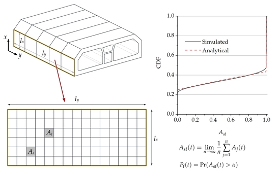
In this section, the initiation time of the corrosion/cracking of a spatially distributed RC structure is considered. Consider a rectangular surface with a size of $l_x·l_y$. Without loss of generality, assume that $l_x\le l_y$. Subdividing the surface into n small cells, as the cell size is small enough, the durability scenario within each cell can be represented by that at a single point within the cell. With this, let a Bernoulli variable $A_i\left(t\right)$ represent the state of the ith cell at time t for $i=1,2,\dots n$, which equals one if failure occurs at the ith cell and zero otherwise. The structural spatial properties such as the concrete cover thickness, chloride diffusion coefficient, and others will affect the sequence $\left\{A_i\left(t\right)\right\}$. Similar to Equation (10), it follows that,

$$\mathrm{Pr}(A_i\left(t\right)=1)=\mathrm{Pr}(T_{*}<t)=F_{T_{*}}\left(t\right)$$

(11)

Figure 2 presents an example of the two-dimensional durability problem, which was adopted from the HZM bridge project. Due to common production process and construction practice [5,40,41], the sequence $\left\{A_i\left(t\right)\right\}$ is spatially correlated (i.e., $A_i\left(t\right)$ and $A_j\left(t\right)$ are correlated for the ith and jth cells), and this correlation is expected to be considered in the estimate of surface durability. The correlation function, denoted by $\rho (\ell )$, is a function of the distance of two locations of interest (ℓ). It by definition equals one when $\tau =0$ and decreases with $\tau$. Different commonly used models are available in the literature to describe the decay behavior of the spatial correlation. For example, if using the exponential law, it follows that,

$$\rho (\ell )=exp\left(-\frac{\ell }{l_c}\right)$$

(12)

in which $l_c$ is the correlation length, at which the spatial correlation equals $exp(-1)\approx 0.368$.

For the whole surface $l_x·l_y$, the limit state typically no longer focuses on the behavior of a single cell (location) only. In fact, many useful indicators for durability assessment use the proportion of failed concrete surface (e.g., with corrosion/crack initiation). Mathematically, the failure of the surface is defined as the scenario that more than $\alpha$ ($0<\alpha <1$) of the whole area is associated with failed performance. Correspondingly, the limit state function for the whole surface at time t is given by:

$$G\left(t\right)=\alpha -\frac{{\int }_0^{l_x}{\int }_0^{l_y}\mathbf{1}\left[t>T_{*}(x,y)\right]\mathrm{d}y\mathrm{d}x}{l_x{l}_y}$$

(13)

where $\mathbf{1}(·)$ is an indicative function, which returns one if the statement in the brackets in true and zero otherwise. Subsequently, according to Equation (1), the time-dependent failure probability at time t, $P_{\mathrm{f}}\left(t\right)$, can be estimated by:

$$P_{\mathrm{f}}\left(t\right)=\mathrm{Pr}(G\left(t\right)<0)=\mathrm{Pr}\left(\frac{{\int }_0^{l_x}{\int }_0^{l_y}\mathbf{1}\left[t>T_{*}(x,y)\right]\mathrm{d}y\mathrm{d}x}{l_x{l}_y}>\alpha \right)$$

(14)

In Equation (14), while an analytical approach was presented for the estimation of surface failure probability, it is practically difficult to implement since the explicit form of the function $\mathbf{1}\left[t>T_{*}(x,y)\right]$ is unknown (which may even take a complicated form). Alternatively, this paper aims to solve Equation (14) based on the discretization of the surface as in Figure 2c. In the presence of n cells as introduced before, let $A_{\mathrm{sf}}\left(t\right)$ be the average performance associated with the surface, that is,

$$A_{\mathrm{sf}}\left(t\right)=\underset{n\to \infty }{lim}\frac{1}{n}\sum _{j=1}^n{A}_j\left(t\right)$$

(15)

With this, Equation (14) becomes:

$$P_{\mathrm{f}}\left(t\right)=\mathrm{Pr}\left(A_{\mathrm{sf}}\left(t\right)>\alpha \right)$$

(16)

If the CDF of $A_{\mathrm{sf}}\left(t\right)$ is $F_{A_{\mathrm{sf}}\left(t\right)}(·)$, Equation (16) is rewritten as follows,

$$P_{\mathrm{f}}\left(t\right)=1-\mathrm{Pr}\left(A_{\mathrm{sf}}\left(t\right)\le \alpha \right)=1-F_{A_{\mathrm{sf}}\left(t\right)}\left(\alpha \right)$$

(17)

and correspondingly, the reliability of the structural surface at time t is $F_{A_{\mathrm{sf}}\left(t\right)}\left(\alpha \right)$.

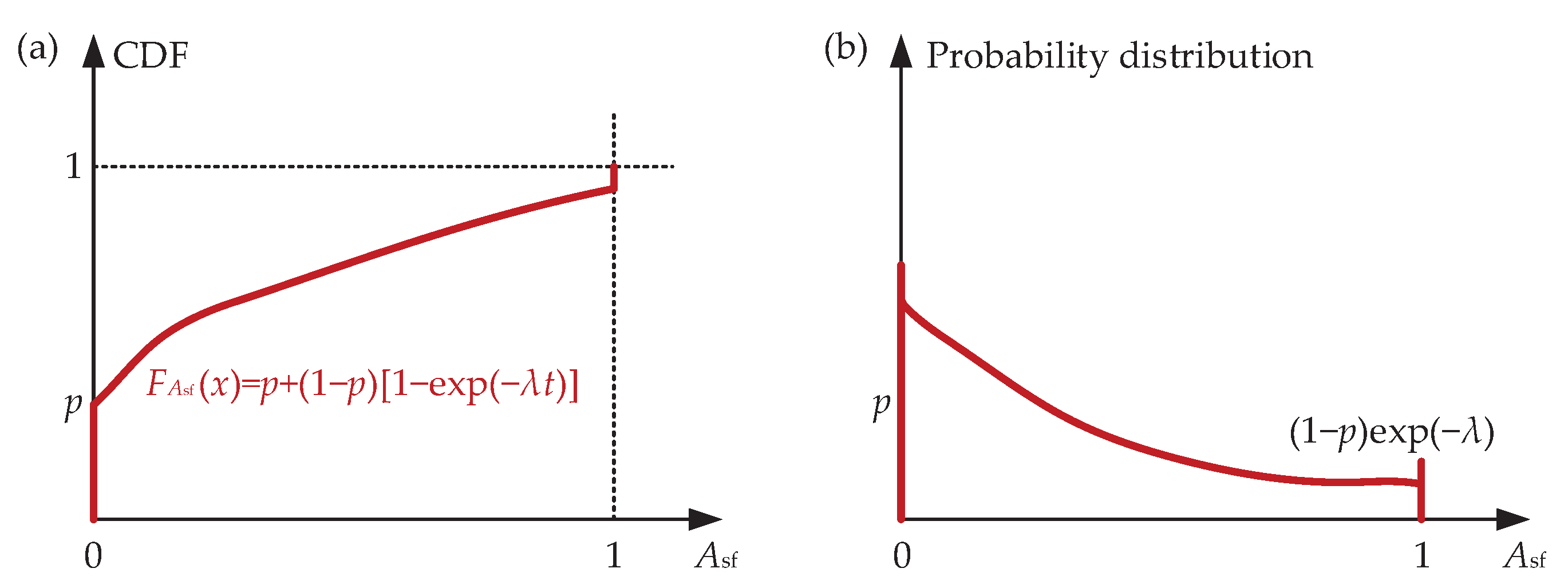
Note that $A_{\mathrm{sf}}\left(t\right)$ is strictly defined within the range of $[0,1]$. This paper proposes to use a mixture distribution to model the probabilistic behavior of $A_{\mathrm{sf}}\left(t\right)$, as shown in

Table 1. Probability distribution of $A_{\mathrm{sf}}\left(t\right)$.

$\mathit{x}=0$	$0<\mathit{x}<1$	$\mathit{x}=1$
p	$(1-p)\lambda exp(-\lambda t)$	$(1-p)exp(-\lambda )$

and Figure 3. Two parameters are involved, namely p and $\lambda$, and will be determined later. In this model, the probability of $A_{\mathrm{sf}}\left(t\right)=0$ equals p (where $0<p<1$), and the probability of $A_{\mathrm{sf}}\left(t\right)=1$ is $(1-p)exp(-\lambda )$. For the range of $(0,1)$, $A_{\mathrm{sf}}\left(t\right)$ is modeled by an exponential distribution with a parameter of $\lambda >0$. With such a configuration, the mean value and variance of $A_{\mathrm{sf}}\left(t\right)$ are respectively:

$$\mu \left(A_{\mathrm{sf}}\left(t\right)\right)=(1-p)\left[exp(-\lambda )+\frac{1-(\lambda +1)exp(-\lambda )}{\lambda }\right]$$

(18)

and:

$${\sigma }^2\left(A_{\mathrm{sf}}\left(t\right)\right)=(1-p)\left[exp(-\lambda )+\frac{2-(2+2\lambda +{\lambda }^2)exp(-\lambda )}{{\lambda }^2}\right]-{(1-p)}^2{\left[exp(-\lambda )+\frac{1-(\lambda +1)exp(-\lambda )}{\lambda }\right]}^2$$

(19)

in which $\mu (·)$ and ${\sigma }^2(·)$ are the mean value and variance of the variables in the brackets, respectively.

The justification for this model is two-fold. First, it aligns well with the overall behavior of $A_{\mathrm{sf}}\left(t\right)$ and provides an easy-to-handle approach to describe $A_{\mathrm{sf}}\left(t\right)$. Second, only two parameters need to be calibrated in this model, which can be done uniquely once the mean value and variance of $A_{\mathrm{sf}}\left(t\right)$ are determined. Noting that the exact solution to the distribution of $A_{\mathrm{sf}}\left(t\right)$ could be very challenging (and may take a complicated form), the proposed model can be used to achieve a tradeoff between the accuracy and efficiency in modeling $A_{\mathrm{sf}}\left(t\right)$. It is shown through a numerical example, in the next section, that the model in Table 1 is reasonably consistent with the realistic distribution of $A_{\mathrm{sf}}\left(t\right)$.

Next, the mean value and variance of $A_{\mathrm{sf}}\left(t\right)$ are discussed. According to Equation (15), for a homogeneous case where the statistics of $T_{*}$ are location-independent, it follows that:

$$\mu \left(A_{\mathrm{sf}}\left(t\right)\right)=\frac{1}{n}\sum _{j=1}^n\mu \left(A_j\left(t\right)\right)=F_{T_{*}}\left(t\right)$$

(20)

In terms of the variance of $A_{\mathrm{sf}}\left(t\right)$, by definition, one has:

$${\sigma }^2\left(A_{\mathrm{sf}}\left(t\right)\right)=\mu \left(A_{\mathrm{sf}}^2\left(t\right)\right)-{\mu }^2\left(A_{\mathrm{sf}}\left(t\right)\right)$$

(21)

Thus, the variance can be easily obtained once $\mu \left(A_{\mathrm{sf}}^2\left(t\right)\right)$ is known. Based on Equation (15),

$$\mu \left(A_{\mathrm{sf}}^2\left(t\right)\right)=\frac{1}{n^2}\mu \left[{\left(\sum _{j=1}^n{A}_j\left(t\right)\right)}^2\right]=\frac{1}{n^2}\sum _{j=1}^n\sum _{k=1}^n\mu \left(A_k\left(t\right)A_j\left(t\right)\right)$$

(22)

Due to the difficulty of computing Equation (22) directly (as it involves the summation of $n^2$ items), the aim of the following derivation is to further simplify Equation (22), which benefited from the method in [42]. Note that the $T_{*}$’s associated with the jth and kth cells, denoted by $T_{*,j}$ and $T_{*,k}$, are mutually correlated. We converted $T_{*,j},T_{*,k}$ into two standard normal variables, $U_j$ and $U_k$, according to:

$$F_{T_{*}}\left(T_{*,j}\right)=\Phi \left(U_j\right),F_{T_{*}}\left(T_{*,k}\right)=\Phi \left(U_k\right)$$

(23)

Let ${\rho }_{U,j,k}$ be the correlation coefficient between $U_j$ and $U_k$. We introduced a normal variable ${\tilde{U}}_{jk}$, which is independent of $U_j$, so that:

$$U_k={\rho }_{U,j,k}{U}_j+{\tilde{U}}_{jk}$$

(24)

The basis for Equation (24) is that, the sum of two normal variables is also normally distributed. Furthermore, based on Equation (24), the mean value and standard deviation of ${\tilde{U}}_{jk}$ are zero and $\sqrt{1-{\rho }_{U,j,k}^2}$, respectively. Based on Equations (11) and (24), it follows that:

$$\begin{array}{cc}\mu \left(A_k\left(t\right)A_j\left(t\right)\right)\hfill & =\mathrm{Pr}\left(T_{*,j}<t\cap T_{*,k}<t\right)=\mathrm{Pr}\left(F_{T_{*}}\left(T_{*,j}\right)<F_{T_{*}}\left(t\right)\bigcap F_{T_{*}}\left(T_{*,k}\right)<F_{T_{*}}\left(t\right)\right)\hfill \\ \hfill & =\mathrm{Pr}\left(U_j<{\Phi }^{-1}\left(F_{T_{*}}\left(t\right)\right)\bigcap {\rho }_{U,j,k}{U}_j+{\tilde{U}}_{jk}<{\Phi }^{-1}\left(F_{T_{*}}\left(t\right)\right)\right)\hfill \end{array}$$

(25)

Using the law of total probability,

$$\begin{array}{cc}\hfill \mu \left(A_k\left(t\right)A_j\left(t\right)\right)& =\sum _x\mathrm{Pr}\left(\left.U_j<{\Phi }^{-1}\left(F_{T_{*}}\left(t\right)\right)\bigcap {\rho }_{U,j,k}{U}_{ij}+{\tilde{U}}_{jk}<{\Phi }^{-1}\left(F_{T_{*}}\left(t\right)\right)\right|U_j=x\right)·\mathrm{Pr}\left(U_j=x\right)\hfill \\ \hfill & ={\int }_{-\infty }^{{\Phi }^{-1}\left(F_{T_{*}}\left(t\right)\right)}\Phi \left[\frac{{\Phi }^{-1}\left(F_{T_{*}}\left(t\right)\right)-{\rho }_{U,j,k}x}{\sqrt{1-{\rho }_{U,j,k}^2}}\right]·\varphi \left(x\right)\mathrm{d}x\hfill \end{array}$$

(26)

in which $\varphi \left(x\right)$ is the PDF of a standard normal distribution. Substituting Equation (26) into Equation (22) yields,

$$\mu \left(A_{\mathrm{sf}}^2\left(t\right)\right)=\frac{1}{n^2}\sum _{j=1}^n\sum _{k=1}^n{\int }_{-\infty }^{{\Phi }^{-1}\left(F_{T_{*}}\left(t\right)\right)}\Phi \left[\frac{{\Phi }^{-1}\left(F_{T_{*}}\left(t\right)\right)-{\rho }_{U,j,k}x}{\sqrt{1-{\rho }_{U,j,k}^2}}\right]·\varphi \left(x\right)\mathrm{d}x$$

(27)

Note that ${\rho }_{U,j,k}$ is a function of the distance between the cells j and k, denoted by ℓ. Thus, ${\rho }_{U,j,k}$ is rewritten as ${\rho }_U(\ell )$. As invoked in [42], one can interpret Equation (27) as the mean value of:

$${\int }_{-\infty }^{{\Phi }^{-1}\left(F_{T_{*}}\left(t\right)\right)}\Phi \left[\frac{{\Phi }^{-1}\left(F_{T_{*}}\left(t\right)\right)-{\rho }_U\left(L\right)x}{\sqrt{1-{\rho }_U^2\left(L\right)}}\right]·\varphi \left(x\right)\mathrm{d}x$$

as $n_i\to \infty$, in which L (a random variable) is the distance between any two points within the rectangular shape $l_x·l_y$. The PDF of L is [43],

$$f_L(\ell )=\frac{4\ell }{l_x^2{l}_y^2}h(\ell )$$

(28)

where:

$$h(\ell )=\left\{\begin{array}{cc}\frac{l_x{l}_y\pi }{2}-(l_x+l_y)\ell +\frac{{\ell }^2}{2},\hfill & \hfill 0\le \ell <l_x\\ l_x{l}_y{sin}^{-1}\left(\frac{l_x}{\ell }\right)-\frac{l_x^2}{2}-l_y\ell +l_y\sqrt{{\ell }^2-l_x^2},\hfill & \hfill l_x\le \ell <l_y\\ l_x{l}_y\left[{sin}^{-1}\left(\frac{l_x}{\ell }\right)-{sin}^{-1}\sqrt{1-\frac{l_y^2}{{\ell }^2}}\right]-\frac{l_x^2+l_y^2}{2}-\frac{{\ell }^2}{2}+l_x\sqrt{{\ell }^2-l_y^2}+l_y\sqrt{{\ell }^2-l_x^2},\hfill & \hfill l_y\le \ell \le \sqrt{l_x^2+l_y^2}\\ 0,\hfill & \hfill \mathrm{otherwise}\end{array}\right.$$

(29)

As a result, Equation (22) is estimated by:

$$\mu \left(A_{\mathrm{sf}}^2\left(t\right)\right)={\int }_{-\infty }^{{\Phi }^{-1}\left(F_{T_{*}}\left(t\right)\right)}{\int }_0^{\sqrt{l_x^2+l_y^2}}\Phi \left[\frac{{\Phi }^{-1}\left(F_{T_{*}}\left(t\right)\right)-{\rho }_U(\ell )x}{\sqrt{1-{\rho }_U^2(\ell )}}\right]·f_L(\ell )\varphi \left(x\right)\mathrm{d}\ell \mathrm{d}x$$

(30)

Since the mean value and variance of $A_{\mathrm{sf}}\left(t\right)$ were readily obtained, one can further compute the two parameters involved in the probability model of $A_{\mathrm{sf}}\left(t\right)$, p and $\lambda$, according to Equations (18) and (19). Subsequently, the reliability (or failure probability) of the surface can be calculated using Equation (17).

The durability assessment method in Equation (17) can also be used to guide the reliability-based inspection and repair strategies for RC structures exposed to chloride ingress, in an attempt to optimize the life-cycle costs associated with the maintenance measures for the structures. In this regard, the dynamic Bayesian network framework can be used to compute the surface reliability provided the inspection results [11,44,45], where the uncertainties associated with the deterioration parameters are reduced and the surface reliability is updated dynamically.

4. Example

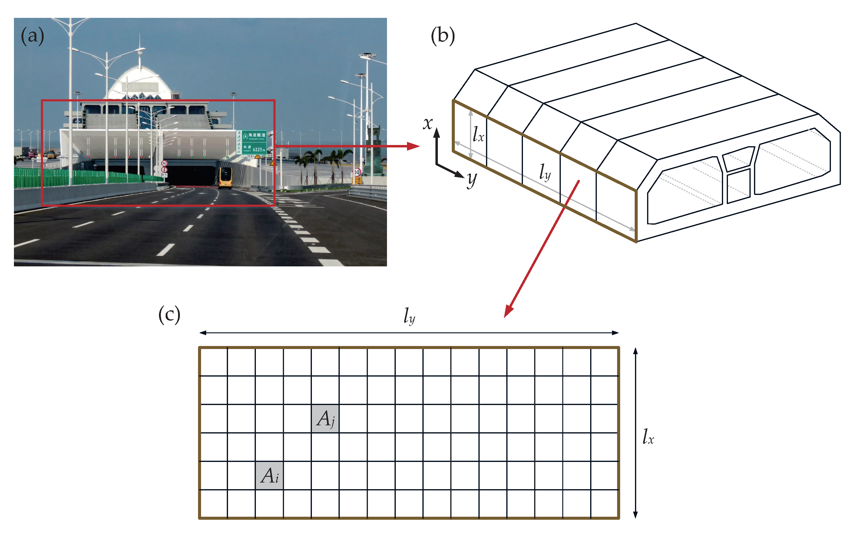
In this section, an illustrative example is used to demonstrate the applicability of the proposed method (cf. Equation (11)). We considered the surface deterioration process of an emerged tunnel tube segment that was used in the HZM project. The corrosion-induced damage scenario on the tube surface was previously studied by Li and Ye [5] using MCS-based methods. We considered a rectangular area with a size of 22.5 m × 4 m, as shown in Figure 2. The concrete compression strength is 50 MPa, and the diameter of the reinforcement bars is 28 mm.

Table 2. Statistical information of the durability parameters.

Phase	Variable	Distribution Type	Statistics	Correlation Length (mm)	Sources
Chloride ingress	$C_{\mathrm{s}}$	Lognormal	mean = 4.5%, COV * = 0.15	2000	[5,10]
	$x_0$ (mm)	Normal	mean = 90, COV = 0.06	130	[5,10]
	$D_{a0}$ (${10}^{-12} {\mathrm{m}}^2/\mathrm{s}$) **	Lognormal	mean = 3.5, COV = 0.35	250	[5,10]
	$n_{\mathrm{a}}$	Normal	mean = 0.47, COV = 0.06	250	[10]
Crack initiation	${\alpha }_0$ in Equation (6)	Uniform	lower = 4, upper = 8	/	[39]
	K in Equation (7)	Deterministic	$0.0366$	/	[5]
	$i_{\mathrm{cor}}$ in Equation (7) ($\mathsf{\mu }\mathrm{A}/{\mathrm{cm}}^2$)	Lognormal	mean = 0.67, COV = 0.58	2000	[5,46]

* COV = coefficient of variation (ratio of the standard deviation to the mean value). ** This diffusion coefficient corresponds to an age of 28 d.

summarizes the statistical information on the relevant durability parameters. In order to reflect the spatial variability and correlation of the parameters, we used an exponential law (cf. Equation (12)) to describe the dependence of the parameter correlation on the distance separation. Assume that the critical chloride concentration, $C_{\mathrm{cr}}$, takes a value of 0.45%, as adopted from [10].

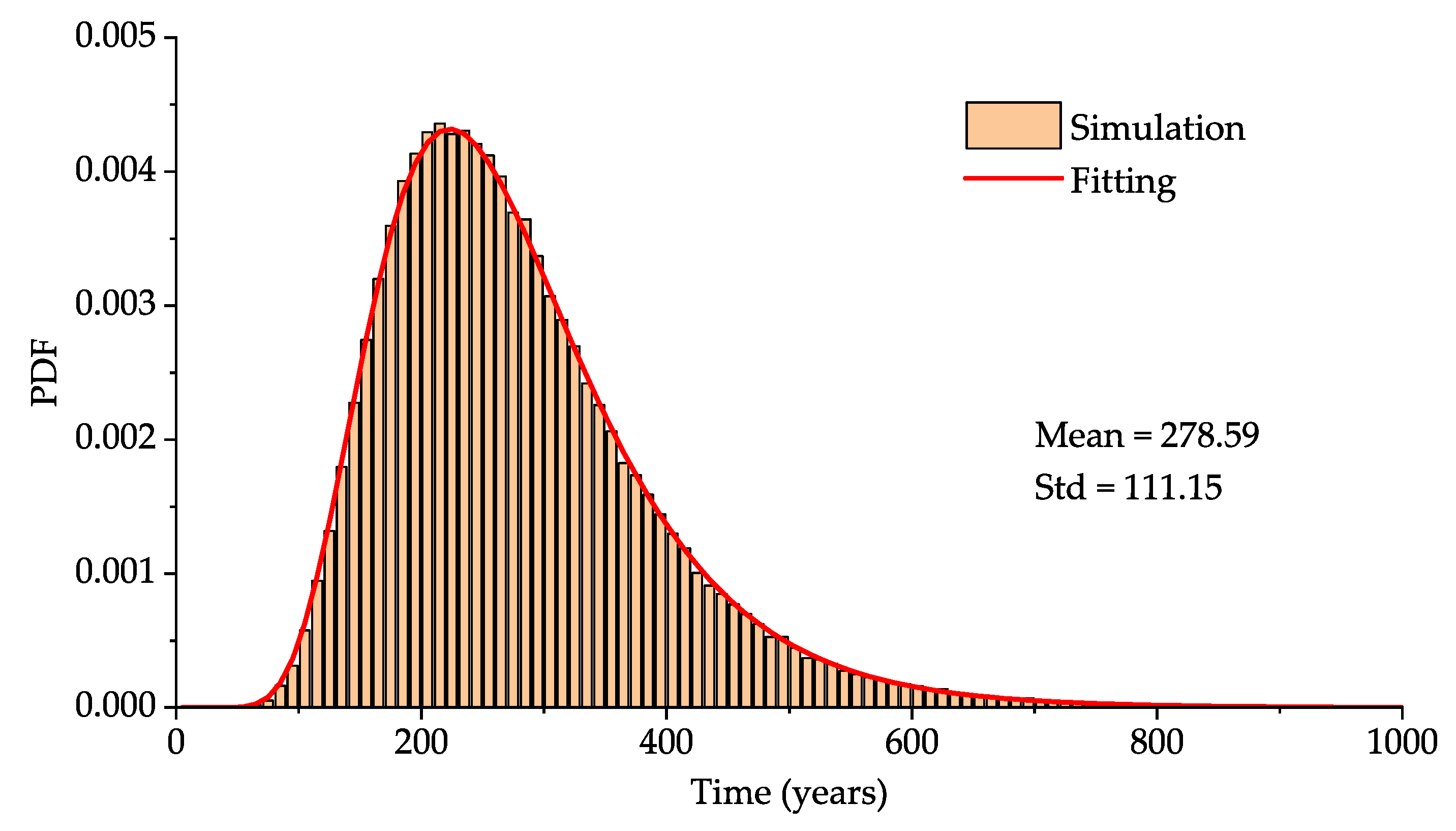
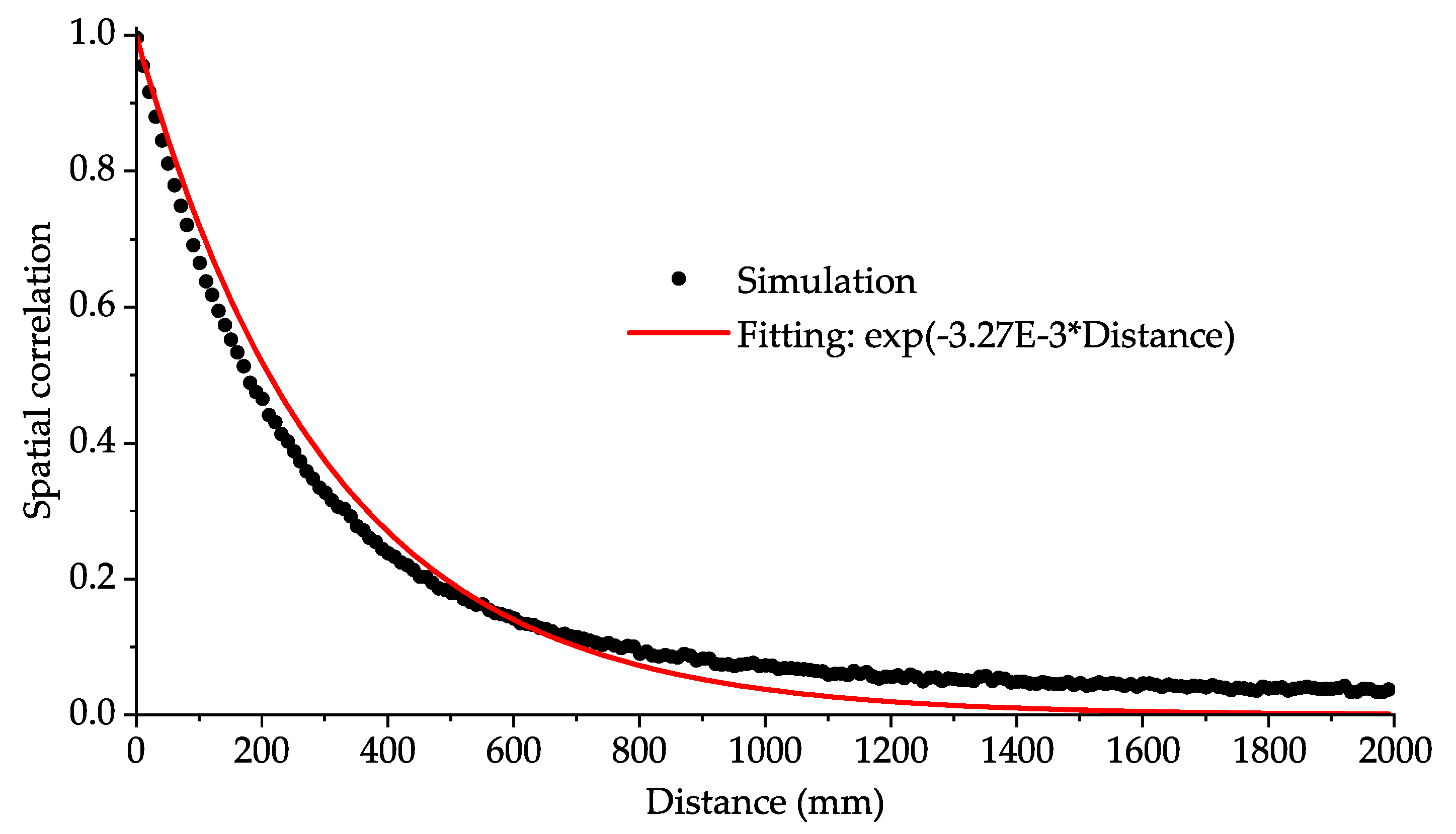
Figure 4 and Figure 5 present the probability distributions of $T_{\mathrm{i}}$ and $T_{\mathrm{ci}}$, respectively, from which it is observed that both $T_{\mathrm{i}}$ and $T_{\mathrm{ci}}$ can be modeled by a lognormal distribution. With the configuration in Table 2, the difference between $T_{\mathrm{i}}$ and $T_{\mathrm{ci}}$ (i.e., $\Delta T_{\mathrm{ci}}$ in Equation (8)) is small, due to the fact that the duration of the first phase (Figure 1) dominates before the occurrence of crack propagation. In fact, the mean value of $\Delta T_{\mathrm{ci}}$ is 19.14 y, which is significantly smaller than that of $T_{\mathrm{i}}$. The spatial correlation of $T_{\mathrm{i}}$ is plotted in Figure 6, which indicates that an exponential law is applicable. The correlation length was found to be 262.8 mm. We emphasize that the correlation fitting of $T_{\mathrm{i}}$ is independent of the service period of interest (t), and thus, the fitting results can be used for durability assessment in the presence of different values of t.

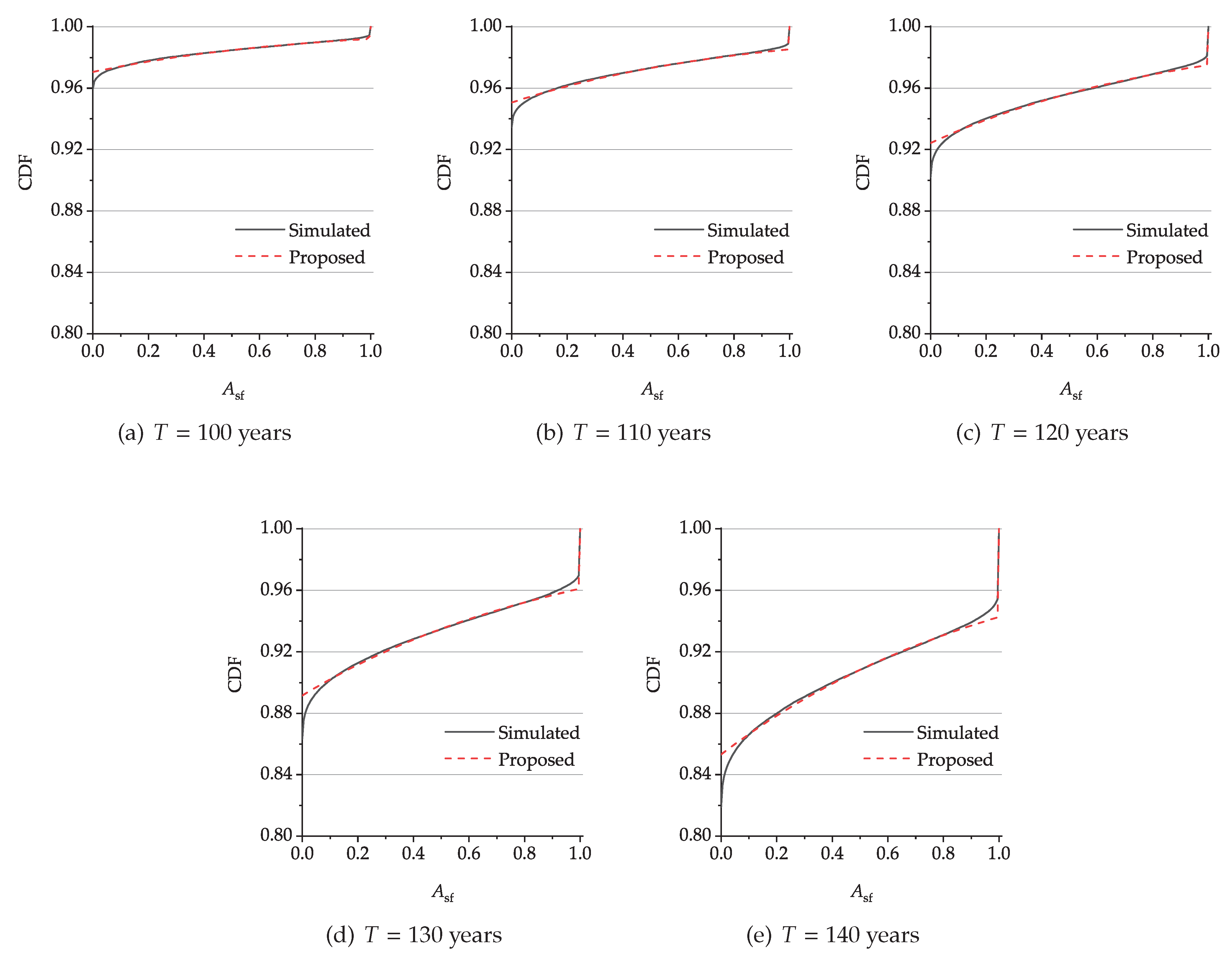
Now, with the information from Figure 4, Figure 5 and Figure 6, one can compute the mean value and standard deviation of $A_{\mathrm{sf}}\left(t\right)$ according to Equations (20) and (21), as shown in

Table 3. Statistics of $A_{\mathrm{sf}}\left(t\right)$ by the proposed and simulation-based methods ($\mu \left(x_0\right)=90$ mm).

Service Life	Mean			Standard Deviation
	Proposed	Simulated	Error (%)	Proposed	Simulated	Error (%)
100 y	0.016	0.016	0.124	0.112	0.111	0.981
110 y	0.029	0.028	0.327	0.149	0.147	1.196
120 y	0.046	0.046	0.035	0.188	0.186	0.899
130 y	0.068	0.068	0.067	0.228	0.226	0.831
140 y	0.095	0.095	0.302	0.267	0.265	0.898

. For a single location, the limit state is defined with regard to corrosion initiation. It can be seen that with an increasing reference period, both the mean value and standard deviation of $A_{\mathrm{sf}}\left(t\right)$ increase with time, which is characteristic of the accumulation of failure risks over time. For comparison purpose, the statistics of $A_{\mathrm{sf}}\left(t\right)$ obtained from MCS (with 100,000 replications) are also presented in Table 3. The comparison between the simulated and analytical results agree well with each other, implying the accuracy of the proposed method. Furthermore, the CDFs of $A_{\mathrm{sf}}\left(t\right)$ from both methods (the proposed and simulated) are presented in Figure 7 for service periods ranging from 100 y to 140 y. For each t, the two results are consistent with each other, indicating that the proposed probability model in Table 1 provides a reasonable estimate of the probabilistic behavior of $A_{\mathrm{sf}}\left(t\right)$. Here, in the simulation, the rectangular area (22.5 m × 4 m) is subdivided into 225 × 40 = 9000 cells. Correspondingly, the size of each cell is 100 mm × 100 mm, which is relatively small so that the durability performance within each cell can be approximated by a single Bernoulli variable. The Nataf transformation method [12,47] was used to simulate correlated random variables.

Based on the CDF of $A_{\mathrm{sf}}\left(t\right)$, the surface failure probability, given a threshold $\alpha$, can be obtained according to Equation (17). Here, a value of 0.01 was considered for $\alpha$ for illustration purpose, coinciding with the Chinese code JTJ 302–2006 [48], which classifies the concrete surface as Grade A if no more than 1% of the surface has visible cracking. The surface failure probabilities associated with the proposed and simulation-based methods are shown in

Table 4. The failure probabilities of the surface obtained by the proposed and simulation-based methods ($\mu \left(x_0\right)=90$ mm).

Service Life	Proposed	Simulated	Error (%)
100 y	0.029	0.034	14.647
110 y	0.049	0.056	13.236
120 y	0.075	0.085	12.101
130 y	0.107	0.120	10.841
140 y	0.145	0.162	10.016

. The accuracy of the proposed method can be verified through a comparison with the MCS results. Furthermore, compared with the failure probability at the material level (cf. Figure 4), the structural durability performance will be significantly overestimated if ignoring the impact of structural geometry. The results in Table 4 were obtained based on the software MATLAB R2019a, using a laptop with the configuration of an Intel(R) Core(TM) i5-8250U CPU @ 1.6 GHz. It took less than 30 s using the proposed method (including the fitting of the distribution type and spatial correlation in Figure 4 and Figure 6); however, when employing the simulation method, it required more than 5 h. This difference indicates that the proposed analytical method is at least 600 times more efficient compared with MCS. Furthermore, if subdividing the surface into more cells (2250 × 400) in the simulation procedure in order to improve the accuracy, an ordinary laptop would become incapable of achieving this goal, as the request of generating a 900,000 × 900,000 (6035.0 GB) array exceeds the maximum array size preference in MATLAB. This fact again shows the advantage of the proposed analytical method compared with MCS.

Note that the probabilistic behavior of $A_{\mathrm{sf}}\left(t\right)$ is estimated in Figure 7 and Table 4 focusing on the initiation time of corrosion. The proposed method is also applicable if considering the time of crack initiation (recall that in Equation (11), $T_{*}$ can refer to either $T_{\mathrm{i}}$ or $T_{\mathrm{ci}}$). Illustratively, consider a case in which the mean value of the concrete cover thickness ($x_0$) is 50 mm, while the other parameters are the same as in Table 2. The proposed method in Equation (17) was applied again focusing on the crack initiation time. First, the probability distribution of $T_{\mathrm{ci}}$ is presented in Figure 8, from which it is observed that a lognormal distribution is suitable for describing the behavior of $T_{\mathrm{ci}}$. The mean value and standard deviation of $T_{\mathrm{ci}}$ are 92.50 y and 35.13 y, respectively. The spatial correlation of $T_{\mathrm{ci}}$ is plotted in Figure 9, suggesting that the exponential decay model (cf. Equation (12)) can reasonably model the correlation of $T_{\mathrm{ci}}$. Subsequently, the statistics (mean value and standard deviation) and the CDF of $A_{\mathrm{sf}}\left(t\right)$ are presented in

Table 5. Statistics of $A_{\mathrm{sf}}\left(t\right)$ by the proposed and simulation-based methods ($\mu \left(x_0\right)=50$ mm).

Service Life	Mean			Standard Deviation
	Proposed	Simulated	Error (%)	Proposed	Simulated	Error (%)
100 y	0.654	0.656	0.306	0.443	0.438	1.084
110 y	0.744	0.746	0.308	0.405	0.400	1.266
120 y	0.814	0.816	0.208	0.360	0.355	1.375
130 y	0.867	0.868	0.125	0.313	0.308	1.531
140 y	0.905	0.906	0.073	0.268	0.264	1.518

and Figure 10, respectively. The comparison with the results obtained from MCS demonstrates the accuracy of the proposed method. Subsequently, the surface failure probabilities associated with both methods (simulation and analytical) are shown in

Table 6. The failure probabilities of the surface obtained by the proposed and simulation-based methods ($\mu \left(x_0\right)=50$ mm).

Service Life	Proposed	Simulated	Error (%)
100 y	0.770	0.747	3.018
110 y	0.841	0.824	2.048
120 y	0.893	0.880	1.451
130 y	0.928	0.919	0.983
140 y	0.952	0.946	0.601

, where $\alpha =0.01$. Consistent with the observations from Table 4, the proposed probability model in Table 1 provides an applicable tool for describing the probabilistic behavior of $A_{\mathrm{sf}}\left(t\right)$, achieving a tradeoff between the accuracy and efficiency in estimating the durability performance of deteriorating concrete surfaces.

5. Conclusions

A closed-form method was proposed in this paper for the durability assessment of RC structures exposed to the marine environment. The method takes into account the spatial variability and correlation of the structural properties such as the thickness of the cover concrete, the chloride diffusion coefficient, and others. For a two-dimensional concrete surface, the mean value, variance, and distribution type of the average durability scenario were derived. The proposed approach provides a link between the durability performance of a structural element and that at the material level. An illustrative example was presented to demonstrate the applicability of the proposed method. The comparison between the analytical results and those from MCS indicated the accuracy of the proposed method. Moreover, it was shown that the use of the proposed method was at least 600 times more efficient compared with MCS, which is beneficial for its practical application.

Note that the proposed method in this paper was examined for the corrosion-induced durability assessment of RC structures based on Equations (5) and (8). It is worthy of future work regarding the method’s applicability in the presence of more complicated deterioration mechanisms with additional differential variables such as the porosity distribution in concrete [49,50].

References

- FIB. Model Code for Service Life Design; Bulletin 34; Fédération International du Béton: Lausanne, Switzerland, 2006. [Google Scholar]
- FIB. Model Code 2010—First Complete Draft; Bulletin 55/56; Fédération International du Béton: Lausanne, Switzerland, 2010. [Google Scholar]
- ISO 16204. Durability—Service Life Design of Concrete Structures; International Organization for Standardization: London, UK, 2012. [Google Scholar]
- CEN. EuroCode2: Design of Concrete Structures (prEN 1992-1-1); European Committee for Standardization: Brussels, Belgium, 2002. [Google Scholar]
- Li, Q.; Ye, X. Surface deterioration analysis for probabilistic durability design of RC structures in marine environment. Struct. Saf. 2018, 75, 13–23. [Google Scholar] [CrossRef]
- Alexander, M.; Beushausen, H. Durability, service life prediction, and modeling for reinforced concrete structures–review and critique. Cem. Concr. Res. 2019, 122, 17–29. [Google Scholar] [CrossRef]
- McGee, R. Modelling of durability performance of Tasmanian bridges. ICASP8 Appl. Stat. Probab. Civ. Eng. 1999, 1, 297–306. [Google Scholar]
- DuraCrete. Probabilistic Performance Based Durability of Concrete Structures: General Guidelines for Durability Design and Redesign; Technical Report, Report No. BE95-1347; CUR: Gouda, The Netherlands, 2000. [Google Scholar]
- Li, K.; Li, Q.; Zhou, X.; Fan, Z. Durability Design of the Hong Kong-Zhuhai-Macau Sea-Link Project: Principle and Procedure. J. Bridge Eng. 2015, 20, 04015001. [Google Scholar] [CrossRef]
- Li, Q.; Li, K.; Zhou, X.; Zhang, Q.; Fan, Z. Model-based durability design of concrete structures in Hong Kong-Zhuhai-Macau sea link project. Struct. Saf. 2015, 53, 1–12. [Google Scholar] [CrossRef]
- Hackl, J.; Kohler, J. Reliability assessment of deteriorating reinforced concrete structures by representing the coupled effect of corrosion initiation and progression by Bayesian networks. Struct. Saf. 2016, 62, 12–23. [Google Scholar] [CrossRef]
- Wang, C. Structural Reliability and Time-Dependent Reliability; Springer Nature: Cham, Switzerland, 2021. [Google Scholar]
- Hong, H. Assessment of reliability of aging reinforced concrete structures. J. Struct. Eng. 2000, 126, 1458–1465. [Google Scholar] [CrossRef]
- Pang, L.; Li, Q. Service life prediction of RC structures in marine environment using long term chloride ingress data: Comparison between exposure trials and real structure surveys. Constr. Build. Mater. 2016, 113, 979–987. [Google Scholar] [CrossRef]
- Wu, L.; Li, W.; Yu, X. Time-dependent chloride penetration in concrete in marine environments. Constr. Build. Mater. 2017, 152, 406–413. [Google Scholar] [CrossRef]
- Stewart, M.G. Spatial variability of pitting corrosion and its influence on structural fragility and reliability of RC beams in flexure. Struct. Saf. 2004, 26, 453–470. [Google Scholar] [CrossRef]
- Li, Y.; Vrouwenvelder, T.; Wijnants, G.; Walraven, J. Spatial variability of concrete deterioration and repair strategies. Struct. Concr. 2004, 5, 121–129. [Google Scholar] [CrossRef]
- Muigai, R.; Moyo, P.; Alexander, M. Durability design of reinforced concrete structures: A comparison of the use of durability indexes in the deemed-to-satisfy approach and the full-probabilistic approach. Mater. Struct. 2012, 45, 1233–1244. [Google Scholar] [CrossRef]
- Stewart, M.G. Spatial and time-dependent reliability modeling of corrosion damage, safety and maintenance for reinforced concrete structures. Struct. Infrastruct. Eng. 2012, 8, 607–619. [Google Scholar] [CrossRef]
- Demis, S.; Papadakis, V.G. Durability design process of reinforced concrete structures-Service life estimation, problems and perspectives. J. Build. Eng. 2019, 26, 100876. [Google Scholar] [CrossRef]
- Vu, K.A.; Stewart, M.G. Predicting the likelihood and extent of reinforced concrete corrosion-induced cracking. J. Struct. Eng. 2005, 131, 1681–1689. [Google Scholar] [CrossRef]
- Akiyama, M.; Frangopol, D.M.; Takenaka, K. Reliability-based durability design and service life assessment of reinforced concrete deck slab of jetty structures. Struct. Infrastruct. Eng. 2017, 13, 468–477. [Google Scholar] [CrossRef]
- Shafei, B.; Alipour, A. Application of large-scale non-Gaussian stochastic fields for the study of corrosion-induced structural deterioration. Eng. Struct. 2015, 88, 262–276. [Google Scholar] [CrossRef]
- Li, C.Q. Life-cycle modeling of corrosion-affected concrete structures: Propagation. J. Struct. Eng. 2003, 129, 753–761. [Google Scholar] [CrossRef]
- Li, C.Q. Life cycle modeling of corrosion affected concrete structures—Initiation. J. Mater. Civ. Eng. 2003, 15, 594–601. [Google Scholar] [CrossRef]
- Yi, Y.; Zhu, D.; Guo, S.; Zhang, Z.; Shi, C. A review on the deterioration and approaches to enhance the durability of concrete in the marine environment. Cem. Concr. Compos. 2020, 113, 103695. [Google Scholar] [CrossRef]
- Bazant, Z.P. Physical model for steel corrosion in concrete sea structures-theory. J. Struct. Div. ASCE 1979, 105, 1137–1153. [Google Scholar] [CrossRef]
- Bamforth, P. The derivation of input data for modeling chloride ingress from eight-year UK coastal exposure trials. Mag. Concr. Res. 1999, 51, 87–96. [Google Scholar] [CrossRef]
- Li, C.Q. Corrosion initiation of reinforcing steel in concrete under natural salt spray and service loading—Results and analysis. Mater. J. 2000, 97, 690–697. [Google Scholar]
- Khan, M.U.; Ahmad, S.; Al-Gahtani, H.J. Chloride-induced corrosion of steel in concrete: An overview on chloride diffusion and prediction of corrosion initiation time. Int. J. Corros. 2017, 2017, 5819202. [Google Scholar] [CrossRef] [Green Version]
- Liu, Y.; Weyers, R.E. Modeling the time-to-corrosion cracking in chloride contaminated reinforced concrete structures. Mater. J. 1998, 95, 675–680. [Google Scholar]
- El Maaddawy, T.; Soudki, K. A model for prediction of time from corrosion initiation to corrosion cracking. Cem. Concr. Compos. 2007, 29, 168–175. [Google Scholar] [CrossRef]
- Mullard, J.A.; Stewart, M.G. Corrosion-induced cover cracking: New test data and predictive models. ACI Struct. J. 2011, 108, 71–79. [Google Scholar]
- Collepardi, M.; Marcialis, A.; Turriziani, R. Penetration of chloride ions into cement pastes and concretes. J. Am. Ceram. Soc. 1972, 55, 534–535. [Google Scholar] [CrossRef]
- Mangat, P.; Molloy, B. Prediction of long term chloride concentration in concrete. Mater. Struct. 1994, 27, 338–346. [Google Scholar] [CrossRef]
- Mangat, P.; Molloy, B. Model for long term chloride penetration in concrete. Mater. Struct. 1994, 25, 404–411. [Google Scholar] [CrossRef]
- Alonso, C.; Andrade, C.; Rodriguez, J.; Diez, J.M. Factors controlling cracking of concrete affected by reinforcement corrosion. Mater. Struct. 1998, 31, 435–441. [Google Scholar] [CrossRef]
- Vidal, T.; Castel, A.; Francois, R. Analyzing crack width to predict corrosion in reinforced concrete. Cem. Concr. Res. 2004, 34, 165–174. [Google Scholar] [CrossRef]
- Gonzalez, J.; Andrade, C.; Alonso, C.; Feliu, S. Comparison of rates of general corrosion and maximum pitting penetration on concrete embedded steel reinforcement. Cem. Concr. Res. 1995, 25, 257–264. [Google Scholar] [CrossRef]
- Engelund, S.; Sørensen, J.D. A probabilistic model for chloride-ingress and initiation of corrosion in reinforced concrete structures. Struct. Saf. 1998, 20, 69–89. [Google Scholar] [CrossRef]
- O’Connor, A.; Kenshel, O. Experimental evaluation of the scale of fluctuation for spatial variability modeling of chloride-induced reinforced concrete corrosion. J. Bridge Eng. 2013, 18, 3–14. [Google Scholar] [CrossRef] [Green Version]
- Wang, C. Explicit Approach for Reliability-Based Design of Lining Structures Subjected to Water Seepage Considering Spatial Correlation and Uncertainty. ASCE-ASME J. Risk Uncertain. Eng. Syst. Part A Civ. Eng. 2021, 7, 04021036. [Google Scholar] [CrossRef]
- Mathai, A.; Moschopoulos, P.; Pederzoli, G. Random points associated with rectangles. Rend. Circ. Mat. Palermo 1999, 48, 163–190. [Google Scholar] [CrossRef]
- Fenton, N.; Neil, M. Risk Assessment and Decision Analysis with Bayesian Networks; CRC Press: Boca Raton, FL, USA, 2018. [Google Scholar]
- Luque, J.; Straub, D. Risk-based optimal inspection strategies for structural systems using dynamic Bayesian networks. Struct. Saf. 2019, 76, 68–80. [Google Scholar] [CrossRef]
- Nakagawa, T.; Seshimo, Y.; Onitsuka, S.; Tsutsumi, T. Assessment of corrosion speed of RC structure under the chloride deterioration environment. In Proceedings of the JCI Symposium on the Analysis Model Supporting the Verification of Longterm Performance of Concrete Structure in Design; Japan Concrete Institute: Tokyo, Japan, 2004; pp. 325–330. [Google Scholar]
- Liu, P.L.; Der Kiureghian, A. Multivariate distribution models with prescribed marginals and covariances. Probabilistic Eng. Mech. 1986, 1, 105–112. [Google Scholar] [CrossRef]
- JTJ 302-2006. Technical Specification for Detection and Assessment of Harbour and Marine Structures; Ministry of Transport of the People’s Republic of China: Beijing, China, 2007. [Google Scholar]
- Zhang, J.; Wang, J.; Kong, D. Chloride diffusivity analysis of existing concrete based on Fick’s second law. J. Wuhan Univ. Technol. Sci. Ed. 2010, 25, 142–146. [Google Scholar] [CrossRef]
- Andrade, C.; Prieto, M.; Tanner, P.; Tavares, F.; d’Andrea, R. Testing and modeling chloride penetration into concrete. Constr. Build. Mater. 2013, 39, 9–18. [Google Scholar] [CrossRef]
Figure 1.
Schematic corrosion-induced deterioration process of RC structures.
Figure 2.
Example of the durability problem. (a) The HZM bridge tunnel (source: https://commons.wikimedia.org, accessed on 14 October 2021, under the Creative Commons Attribution-Share Alike 4.0 International license). (b) A segment of immersed tunnel tube used in the HZM project (after [5]). (c) Discretizing the two-dimensional surface into small cells.
Figure 3.
Illustration of the probability distribution of .
Figure 4.
Probability distribution of .
Figure 5.
Figure 6.
Spatial correlation of .
Figure 7.
CDFs of by the proposed and simulation-based methods ( mm).
Figure 8.
Probability distribution of with mm.
Figure 9.
Spatial correlation of with mm.
Figure 10.
CDFs of by proposed and simulation-based methods ( mm).