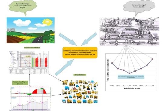
Dynamic Planning of Construction Site for Linear Projects


Faculty of Civil Engineering, Aristotle University of Thessaloniki, 54124 Thessaloniki, Greece
*
Author to whom correspondence should be addressed.
Infrastructures 2021, 6(2), 21; https://0-doi-org.brum.beds.ac.uk/10.3390/infrastructures6020021
Submission received: 17 December 2020
/
Revised: 25 January 2021
/
Accepted: 27 January 2021
/
Published: 1 February 2021
Abstract
:The area of dynamic planning of construction sites is unexplored. Although there is a large amount of scientific interest in the literature in dynamic planning of construction site layouts, with different methodologies developed, studies on construction site relocation do not exist. The purpose of this study is to cover this gap in the literature and contribute to the body of knowledge by presenting for the first time a dynamic planning of a construction site and its importance in linear construction projects and to validate this methodology through real case studies. The decisive variables that determine the appropriate site locations and the costs that arise from these choices are analyzed. The choice that maximizes the production rate of the construction site and thus minimizes the costs is further investigated. An algorithm has also been developed that estimates the cost of transportation of the equipment used in the project and thus enables the investigation of the “ideal” location that minimizes this cost. The “ideal” site location is examined according to the time schedule of the project at time intervals that are determined by the work progress. The optimization algorithm aims to minimize the cost that derives from non-productive activities. The validity of the proposed model is tested in four motorway projects. A sensitivity analysis concerning different sequences in the construction methods reveals remarkable changes in cost fluctuations depending on project size. The outcomes show that for the second, third, and fourth projects, dynamic planning is demanded, and the profit gained ranges from 1 to 1.5% of total budget cost. Financing expenses could be covered by this profit. The case studies presented are derived from linear infrastructure projects that are more sensitive to this approach because of their size and their budget that both affect the results.
1. Introduction
Dynamic planning of a construction site is established in the context of this study as the procedure that searches for the locations that minimize transportation costs of resources in linear projects according to a time schedule. Relocation of a construction site is a critical factor that can increase the productivity of a project. Poor planning when choosing a site installation results in increased transport costs, inefficient use of resources and an increase in non-productive time. The dynamic planning of a construction site is an unexplored part of the construction process of a project. The purpose of this study is to highlight this unexplored issue as well as to investigate the impact of the relocation of the site on the total cost of the project.
Until now, studies have been mostly focused on the effective placement of construction site layouts within the construction site and on their possible relocation after some time in order to enhance both productivity and safety [1]. This concept has been approached through different methodologies with remarkable success, yet without considering the effect of a possible site relocation on the total cost of construction, safety and project duration. In the past few decades, many researchers have focused on the potential use of information technology in the 4D simulation of site layout planning. Digital technologies such as artificial intelligence [2,3], virtual reality [4], building information modeling (BIM) [5,6,7], Darwinian evolution theory [8], binary-mixed-integer-linear program [9], and genetic algorithms [10,11] can be widely applied to optimize construction site layout planning.
This study investigates all possible construction site locations location, which is a very challenging task due to the large number of different qualitative and quantitative parameters involved. Potential benefits of these locations are explored according to the changing needs that arise from project progress. Based on the quantitative criteria, the location of the site corresponding to the lowest cost is chosen. If this position also satisfies the quality restrictions (morphology and soil quality, soil slope, accessibility, legislation, available water supplies, electricity, etc.) then it is finally chosen as the ideal location for construction site installation. An optimization algorithm is proposed with respect to the total construction operating costs by quantifying the combined effect of the cost variables involved. The algorithm is applied on four different motorway projects, and the results are promising; the profit of a dynamic relocation could cover financing costs and thus ensure the viability of the project [12,13]. A sensitivity analysis is carried out to address the extent of different construction methods on the proposed algorithm.
2. Literature Review
2.1. Scientometric Analysis
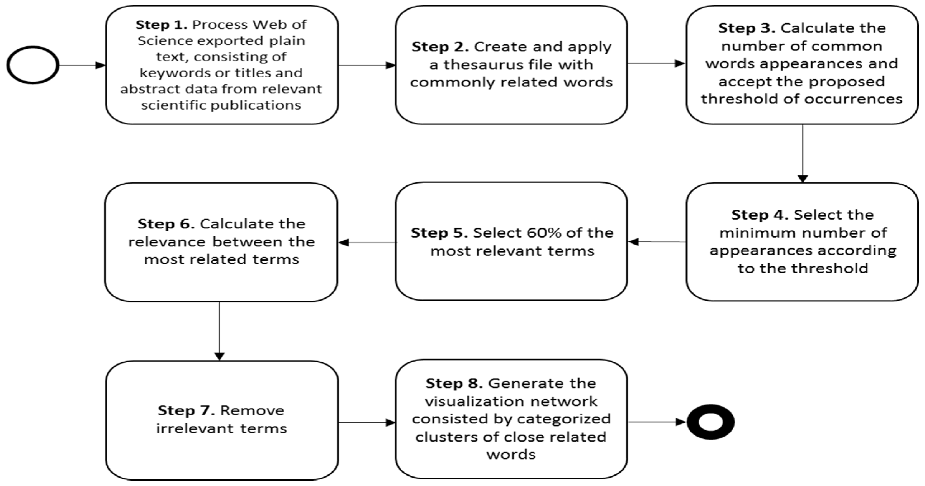
A scientometric analysis was used to search studies on dynamic construction site relocation. This analysis involves searches in the literature by applying the method of “science mapping”, which acts as both a descriptive and a diagnostic tool for research policy purposes, processing immense reservoirs of bibliometric data [14]. As a broader approach, the scientometric analysis covers bibliometric methods, tools, and data to assess the literature. A wide range of science mapping tools for bibliographic analysis are available [15] for mapping and visualizing a particular large-scale scholarly dataset in a knowledge domain [16]. Van Eck and Waltman [17] presented for the first time their text mining computer program for creating, visualizing, and exploring bibliometric maps of science, called Visualization of Similarities Viewer (VOSViewer). It can be used for analyzing all kinds of bibliometric network data, for instance, citation, co-citation, bibliographic coupling, keyword co-occurrence, and co-authorship networks [18]. Science mapping, in the present study, was performed in six consecutive text mining steps, as shown in Figure 1.
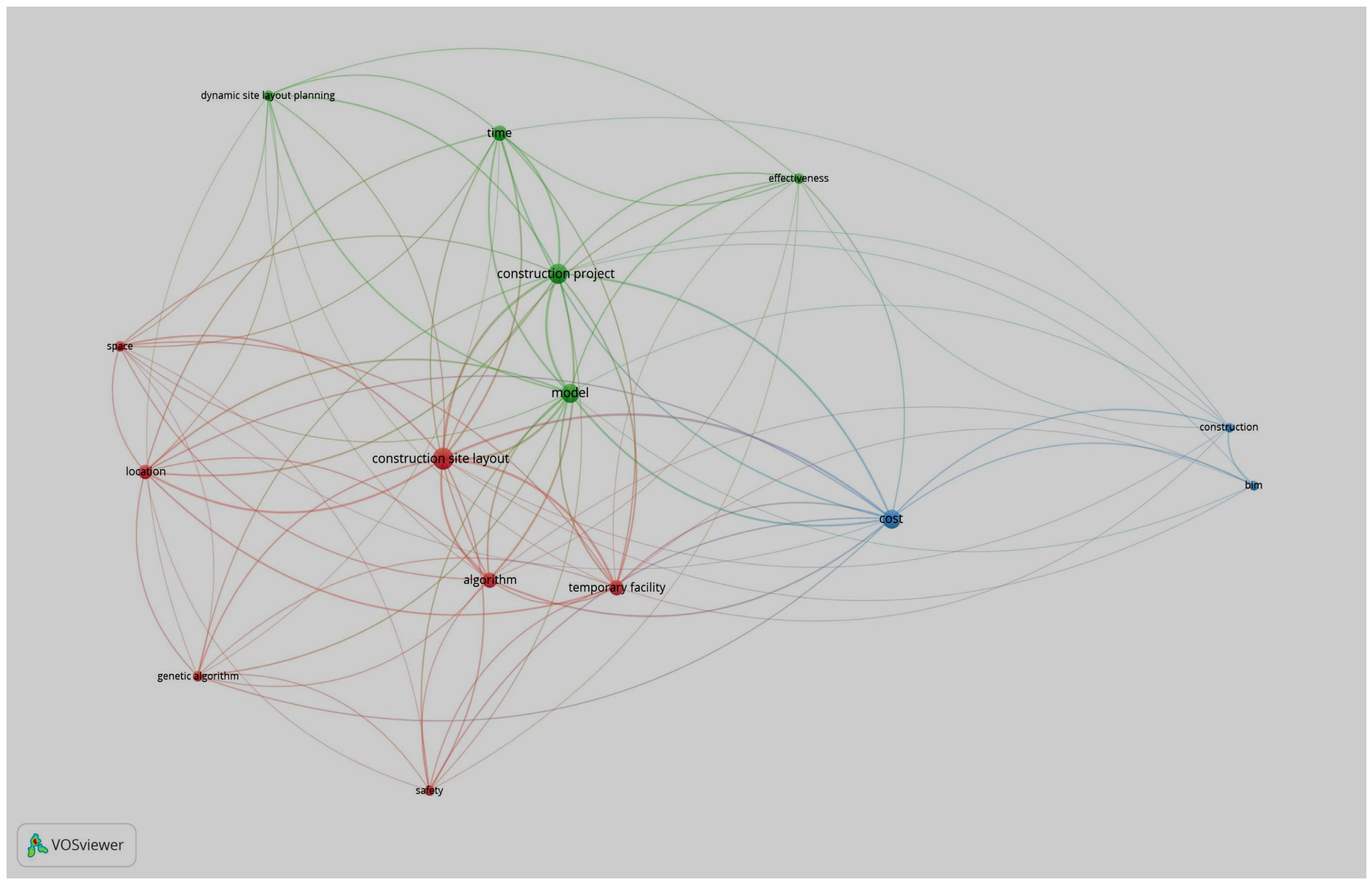
The process starts with the extraction of keywords, titles, and abstracts generated from the scientific publications published in Web of Science (WoS) and Scopus for the last 26 years from 1994–2020. The text mining process in VosViewer for the analysis of co-occurrence relations between scientific terms consists of using word similarity functions to output a graph with clusters of these words. This process is presented in Figure 2, where a visualized map of keyword co-occurrence based on bibliographic data is created. Before the analysis, a thesaurus file was created in order to merge different variants of a keyword, which could appear in many ways; for example, “site layout” and “site” were replaced by “construction site layout”. The total number of terms was 647, but with a minimum number of occurrences of 6, only 15 met the threshold.
In the last step of the text mining process, similar words were clustered together (as represented by the different colors), classified as main research areas, and given a specific name. Within a given cluster, words were ranked based on the number of publications in which they were found. This was reflected by the size of the circle for each word. The distance between the circles provides an indication of relatedness, so that the closer the circles, the higher the relatedness of the words. The colors were assigned automatically and range from red to green, blue, and yellow. The degrees of relatedness between words is indicated by the curved lines. The number of word occurrences in each cluster is given in Table 1.
The clusters show 3 centric thematic areas: cluster 1, Construction site layout; cluster 2, Construction project; cluster 3, Construction. In the first and second cluster, dynamic relocation of site facilities is approached through the relevant terms, whereas in the third cluster, building information modeling (BIM) is presented in the literature and reveals that dynamic site facilities relocation is dealt with by the research community through BIM technologies; the first encountered research was published in 2014. What is evident and important through this in-depth approach is that our research comes to cover the void in the literature and presents an algorithm that proposes the optimal construction site locations with the minimum transportation cost for construction equipment for linear construction projects.
2.2. Literature Review on Dynamic Construction Site Facilities Relocation
Elbeltagi et al. [2], by combining artificial intelligence tools, modeled a system that depended on the schedule for site space allocation. Such a system offered optimized site layout alternatives for different construction phases. Papadaki and Chassiakos [1] developed a multi-objective optimization model aiming at minimizing a generalized cost function, which results from the construction cost of a facility placed at alternative locations, the transportation cost between locations, and any safety concern in the form of preferred proximity or remoteness of facilities to other facilities or work areas. Genetic algorithms were used for the optimization process. Zouein et al. [19] presented a construction algorithm to solve the constraint dynamic layout problem. The optimization formulation aimed to minimize transportation and relocation costs of resources that were subject to 2D geometric constraints; resources were represented as rectangles whose dimensions might or might not vary over time. Minimizing overall security risks and overall costs were the targets of the research presented by Said and El-Rayes in 2010 [20]. Their framework was developed in four main phases: (i) risk identification and system modeling, (ii) security lightning optimization, (iii) security-cost optimization, and (iv) performance evaluation. Cheng and Yang [21] developed an automated site layout system that assists the project manager in identifying suitable areas to locate temporary facilities in order to increase construction productivity. Elbeltagi et al. [22] combined productivity issues and safety in construction sites. This prototype system was demonstrated through a case study of a methodology for site layout planning that combines the effect of safety, productivity, construction site area, and the interrelationships between the necessary facilities on the total operating costs. In 2012, Xu and Li [23] proposed a fuzzy random multi-objective decision-making model to minimize the total cost of site layout and maximize the safety in the construction plant. Andayesh and Sadeghpour [24] developed an innovative dynamic model that could generate layouts that are optimized over the duration of the project. The model applies energy principles governing a physical system to search for the optimum location of objects. Said and El-Rayes [25] developed a multi-objective optimization analysis for planning construction site layouts and site security systems for critical infrastructure projects, trying to minimize security risks and construction costs. Tam et al. [26] proposed a nonstructural fuzzy decision support system that integrates expert judgment into computer decision modeling. Li and Love [27] used genetic algorithms to solve the site-level facility layout problem while satisfying layout constraints and requirements. Yeh [28] proposed the use of annealed neural networks, merging the features of simulated annealing and the Hopfield neural networks. A BIM-based construction layout planning framework was proposed by Cheng and Kumar; the authors used the information from BIM models and produce a dynamic layout model for facility layout optimization to minimize the transportation distances for personnel and equipment [29]. For large-scale construction projects where the complexity of construction site layouts is even greater, Al Hawarneh et al. [30] proposed in their work a grid layout model to accommodate safety as a design parameter beside cost based on safety proximity level between facilities.
The effect of the construction site location on the total operating cost of the construction site remains an unexplored area. This work aims to fill this gap in the research by investigating how the relocation of the construction site minimizes the total cost of a project by minimizing the transportation cost of construction equipment. The focus is set on identifying the “ideal” location. The construction project is examined in sub-periods according to the time schedule, and the search for the “ideal” location begins through an optimization algorithm that minimizes the transportation costs of the construction equipment. The algorithm is repeated in the consecutive sub-periods for the whole project. The algorithm is tested in four different motorway projects that have been already constructed to validate its potential. Construction schedules in accordance with different location scenarios are explored. Finally, a sensitivity analysis is performed to address the extent of different construction methods on the algorithm. The results indicate that the proposed model provides effective and rational solutions in response to decision parameters and problem constraints, as is explained in in more detail the following paragraphs.
3. Dynamic Optimization Module
3.1. Decision Variables for Site Location
The first and most important variable of site layout planning, which contributes significantly to decisions in reference to site logistics, is the size and the location of the site [31]. According to Greek Building Regulation [32], there are several requirements regarding the available locations for site construction. These requirements include the following decision variables [33,34,35]:
- Free locations for site layouts (including regulatory factors such as the use of land, archeology, biodiversity, etc.) [36].
- Electricity, water, and sewage supply systems.
- Ground morphology suitability [31].
- Environmental conditions of the area [33].
- Ground slope. Slopes that are more than 17% are considered unsuitable because of the high grade of resistance in the movement of the equipment that means higher transportation cost and waste of time [32].
Locations should fulfill all of the requirements above in order to be suitable for construction sites, and therefore; these locations are included in the optimization model.
3.2. Cost Parameters/Factors
Construction site layout planning is an important part of project success [37]. An effective construction layout plan can enhance the performance of the construction process by improved productivity, ensured safety, and minimized costs. Especially in linear projects, the aim to be close to the construction activities could minimize even more the transportation costs and guarantee improved productivity. Therefore, the profit of a dynamic construction site layout could cover financing costs following the project timeframe. The following cost parameters/factors could indicate the “ideal” site location by minimizing the overall operating/transportation cost. According to the literature and the interviews conducted by the authors with the projects managers of the cases studies presented with an experience of more than twenty years in the field of public highway construction in Greece, the parameters that should be considered for the appropriate location of a construction site are the following:
- Transport costs of workers and machinery to the working area. The cost-effectiveness of this variable becomes higher for long linear projects.
- Cost of truck and tank operator due to travel to and forth the construction site (transportation of soil, inert, asphalt, water, refueling of project machinery, etc.).
- Fuel costs of trucks and tanks due to transport to and from the construction site.
- Duration of transportation for work. If the duration of transportation from the construction site to the workplace is long, then the production rate drops [38].
- Slope effectiveness. For steep slopes above 10% but below 17%, a modulation of the ground would be necessary.
- The influence of the morphology and the quality of the ground on the total cost (loose sand, clay, sludge, etc.). In case the ground is not suitable to host heavy facilities, soil reinforcement should be applied.
- Accessibility of construction site by trucks hauling material deliveries, fire trucks, ambulances [39].
- Accessibility from the construction site to the working area. In case there is no access, temporary site roads should be constructed.
- A minimum profit. This is an amount set by the contractor for which he would proceed with a relocation (for the purposes of this study, this marginal profit was taken equal to zero).
- Distance from neighboring infrastructure (negative rating scale) (<100 m, 100 m–1 km, >1 km).
3.3. Presentation of the Optimization Equation/Objective
The total transportation cost (TC) considers five factors as presented in formula (1). Costs that emerge from the transportation of equipment and tanks from site to working area and vice versa are the unproductive hourly cost of equipment operators, costs related to the construction of site road network are taken into account as depicted in the following equation [35,38]. The first refers to the transportation cost of the machinery and tanks from the construction site to the working site (and vice versa), while the second refers to the unproductive time due to worker’s transportations. The rest of the factors include costs related to ground formation, slope leveling, and construction of the road network, as shown below:
where
- i: chainage of the controlled “ideal” location (m);
- x: the chainages of the worksites in which the project is divided (m);
- tp: the time period, for which the quantities are taken into the calculation;
- Transportationx,tp: the total number of necessary transportations from the construction site (i) to the work site (x) for the machinery (trucks, excavator, concrete mixer) to execute a task, within the examined time period. This factor is the result of the quantities (m3) for every task divided with the capacity (m3) of the trucks;
- fuel consumption: the fuel consumption of each machine(lt/km);
- machinery speed: the speed of the machine (km/h);
- fuel cost the cost of the necessary fuel that is used for the function of the machines, to execute the demanded tasks in the examined time period ( €/lt);
- hourly wage: the average wage that the workers are paid per hour of work ( €/h);
- GRcosti: the cost that is necessary in case that ground reinforcement is demanded ( €);
- Sli: the cost that is necessary in case that slope leveling is demanded ( €);
- RCi: the cost for the construction of the road service network ( €);
For example, Table 2 shows the work quantities for a random chainage position (i = 18 + 450). In order to apply Equation (1), the necessary movements of vehicles (number of transportation trucks) for the transport of materials from the chainage position i = 18 + 450 to the site installation site (Table 3) are initially calculated. The number of work quantities’ movements depends on the capacity of the company’s available machinery for the project. For each project, the available equipment is determined early in the project.
For example, if the machinery was stored on the worksite and there were no transportations to the construction site, and, given that the price of fuel was estimated based on market prices at 1.50 €/L, the operator’s wage was estimated at 80 €/day, the average speed of trucks was taken 35 km/h and average fuel consumption was 60 L/100 km based on previous data of companies’ fleet management and the manufacturers’ handbooks, then Equation (1) is calculated as follows:
If x = 14 + 850 (the middle of the project), then TC(14 + 850, whole project)18+450 = 5771.10 €.
According to the above formula, the total cost of the tanks and trucks is calculated for each possible site location. The “ideal” location for the project, as a whole, is calculated by determining the sum of the total movements of the tanks and trucks. This calculates the total movements of the project. The ideal site location is where the total movements of the project are shared. The same process is carried out for each period of work (i.e., the time period that the site manager selects to divide the project schedule according to important milestones) and for any possible combination of consecutive periods.
3.4. Description of the Optimization Algorithm
Depending on the accuracy that a project manager would choose, the project is divided into time periods; these time periods is identified with the minimum time period in which the project manager would accept to proceed with a possible relocation (i.e., after the first semester and the combination of the semesters until the end of the project duration). Accordingly, the density of the chainages in which the project is divided is defined, and the works quantities are measured (e.g., every 100 m). The time period for a possible relocation is set 6 months or 1 semester for projects 1, 2, and 4 and one year for project 3. The total quantities of the materials (e.g., concrete, steel, culverts) are divided into work areas with chainages increasing per 100 m. The “ideal” location of the construction site is calculated not only for every semester/year (1, 2, 3, …, N), but also for the combination of non-overlapping semesters/years [1 + 2, 1 + 2 + 3, 2 + 3, …, N + (N + 1)]. Every different combination of non-overlapping semesters/years constitutes a scenario. Finally, the total cost for each scenario is compared with the total transportation cost of the whole project. The minimum TC corresponds to the “ideal” scenario. Table 3 presents the aforementioned process.
For instance, scenario X examines one relocation of the construction site at the end of the Nth time period. For the first time period, which starts at the beginning of the project and ends at the Nth semester, the construction site is established at the available location a, which is the “ideal” location for this period. The operating cost for this period and for this “ideal” location would be ‘A’ €. In addition, the relocation of the construction site is added. The relocation (R) cost represents the actual cost of moving the facilities from the first location to the other [37]. For the second time period, which lasts from the beginning of (N + 1)th the semester until the end of the project, the construction site is established at the available location b, which is the “ideal” location for this period. The cost for this period at the “ideal” location would be B. User’s Target ( €) is the amount that the project manager would like to achieve in order to proceed with the relocation of the construction site. Summing up all the aforementioned costs for scenario X (A + R + B + user’s target), profit or loss compared to the base scenario is entailed. The above process is presented in Table 4.
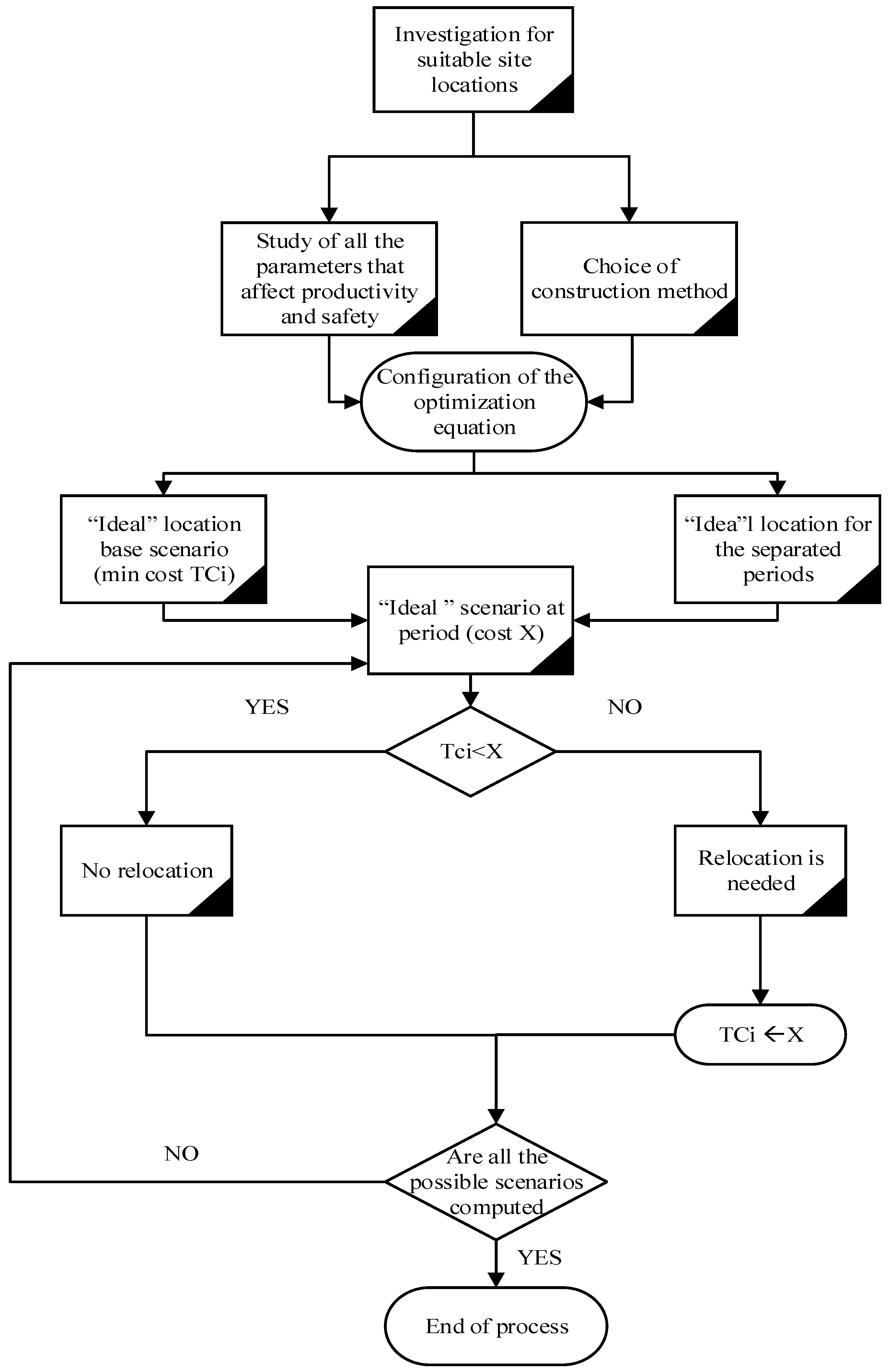
The “ideal” scenario may include 2 or more relocations in order for all the possible combinations of non-overlapping time periods to be investigated. The optimization algorithm is presented in Figure 3. The algorithm ends when all the possible combinations are investigated and the best scenario is promoted.
4. Performance Evaluation of the Model
4.1. General Description of Case Studies
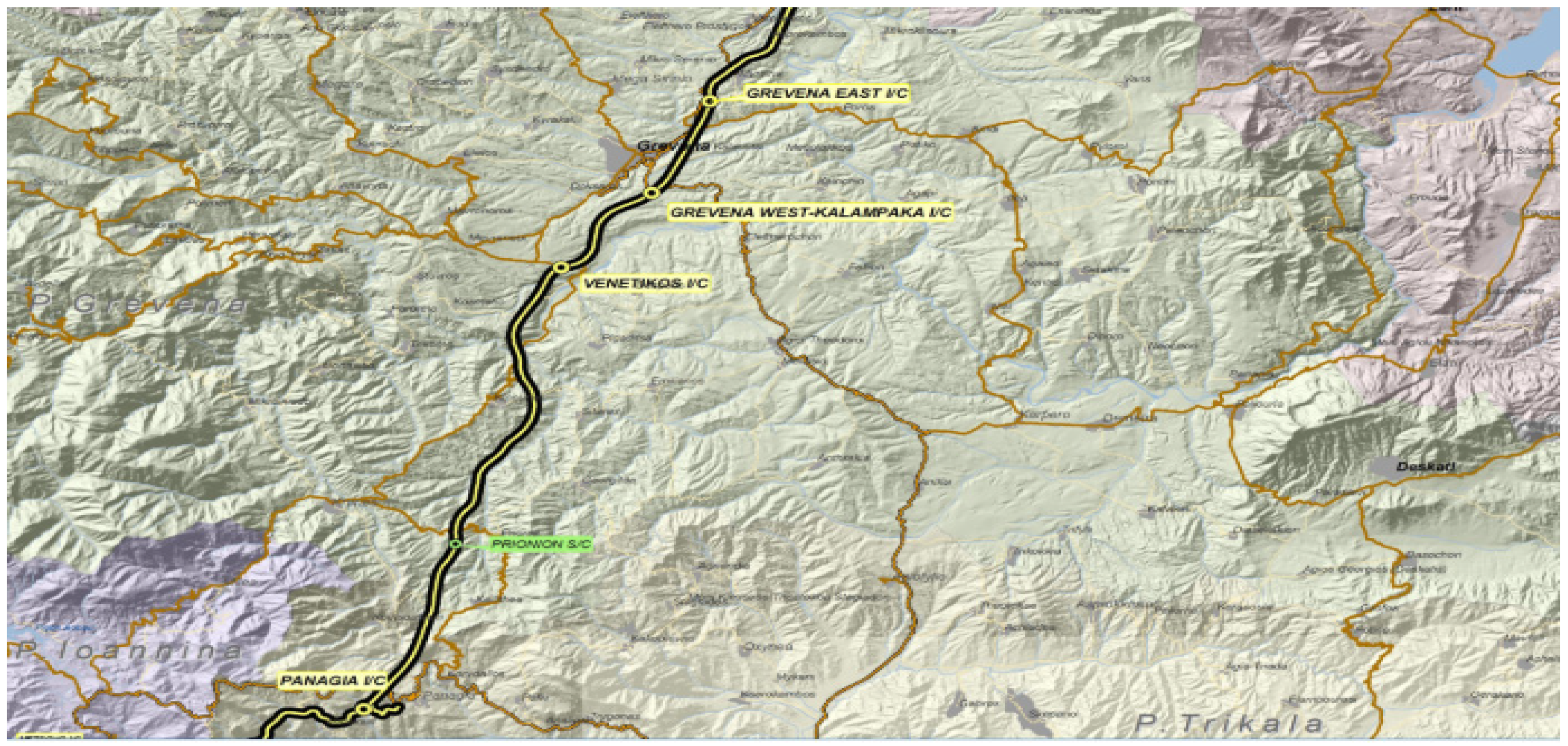
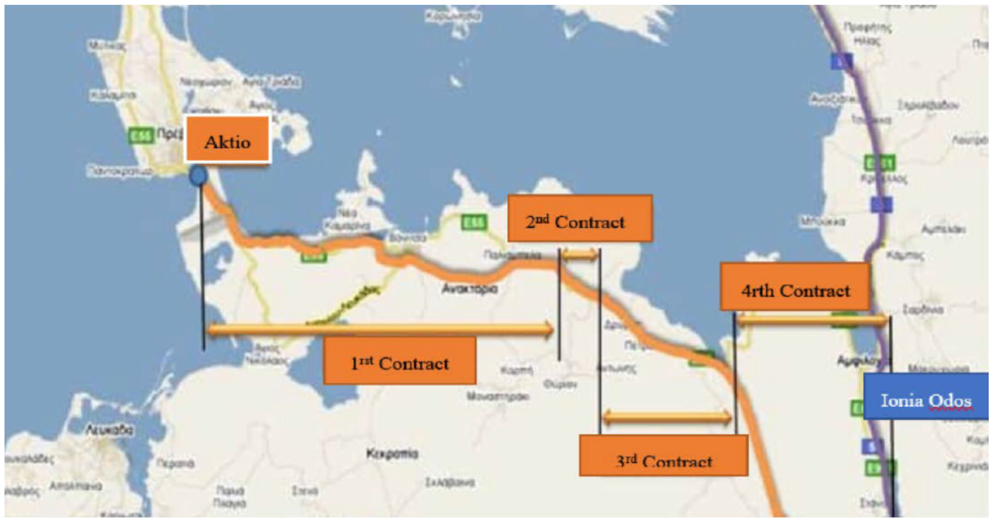
The model has been implemented into four motorway projects; the first project is a small vertical axe of Egnatia Odos Motorway in North Greece with a length of 5.5 km and a total cost of 25,000,000 €. The construction duration was three years from 2015 to 2018. The second project is a part of Egnatia Odos Motorway 15 km long (Scheme 1) and a total cost of 127,000,000 €, and the construction phase of this project also lasted 3 years from 2004 to 2007. The work quantities of material were calculated for every 100 m, and the project duration was divided into semesters. The third examined project was a part of the motorway from Amfilochia (east part of the motorway) to Vonitsa (west part of the motorway) (Scheme 2). The construction of the motorway was made under four contracts, and the case study presented is concerned with the work executed under the first contract (Scheme 2). The total length of the project was 22.5 km, and the total cost was 120,000,000 €. The examined part extends from chainage 0 + 000 to 22 + 500. Following the contractor’s execution methodology of the constructor, project machinery (i.e., excavators, loaders, graders) was stored on-site, the products of the excavation were used for the embankments, and there was a concrete and asphalt plant for technical works and pavement. The total duration of the project was 8 years (eight time periods). The work included excavation, embankments, asphalt paving, technical works, tunnels, and bridges. The fourth examined project refers to the construction of the remaining works of the motorway from Amfilochia to Vonitsa, which were not completed under the original contracts. The construction time of the project was from 2019 to 2021, with a total length of 30.9 km and a cost of approximately 54,000,000 €. The available data for this project were the project schedule, information on how the site works, construction provisions, human resources, and available machinery. In this project as well, the quantities of material were calculated for every 100 m, and all possible scenarios of joint operation of a construction site were examined.
Microsoft Excel was used to store data in a sequence flow according to the 100 m advancement rate, and the optimization process of Equation (1) was performed using Evolver 7.5.2 of Palisade. The minimum cost is represented by the “ideal” location for each scenario. The input data necessary concern the length of the project, the daily advancement rate of works, the volumes of excavations, the machinery used and their operating characteristics (capacity, production rate, hourly cost, fuel consumption, etc.), number of operators and their hourly cost, and fuel price. After entering the required information, the process of automatic calculation begins. The software automatically performs the calculations to indicate the required movements in each scenario that create the minimum cost.
According to the presented algorithm, a profit of approximately 100,000 € to 186,000 € was created for the second, third, and fourth projects, respectively. Project size determines site layouts, which in turn define the relocation cost. According to projects managers of the projects presented, for a typical linear project, relocation cost could range from 20,000 € to 34,000 €. Through a sensitivity analysis conducted, where different construction methods were applied and changes in macroeconomics factors were made (fuel’s price, operators’ wages), very interesting qualitative conclusions were derived.
4.2. Analysis and Results of Case Study 1
The project manager stored machinery at the site, excavation quantities were not used for embankments.
The available machines for this project and their exact number as used for each task are as follows:
- 2 excavator (with a bucket capacity of 2.40 m3)
- 2 loaders (with a bucket capacity of 3.50 m3)
- 1 crane truck
- 4 earthmoving trucks
- 4 road trucks
- 2 asphalt trucks
- 2 pavers
- 1 finisher
- 1 water tank
The excavator was for work on soil excavations; the loader was to load them; earthmoving trucks were to remove soil from the project; road and asphalt trucks were for the transport of the above materials from the construction site to the workstation; the paver was for the condensation of the soils, base, background and asphalt; the finisher was for the paving of asphalt and water tanks for the transport of water to the worksite. The price of fuel was considered 1.50 €/L and the operator’s wage 80 €/day.
According to this works profile, no relocation of construction site was necessary with an operating construction cost at 104.507,36 €.
Table 5 presents the total operating costs as they are generated by the application of the mathematical Equation (1), according to the examined location. The first column presents the scenarios, the second column depicts the semesters of the executed work. The fourth column indicates the operating cost of each scenario, and the last column calculates the profit or loss of each scenario compared to the cost of the “ideal” location for the base scenario. The “ideal” location for the entire project is at chainage i = 2 + 650, and the cost of construction site is TC(i=2+650) = 104,507.36 €. Ιn the first scenario, the “ideal” location for the quantities of 1st to 3rd semester is i1 = 3 + 050, and the cost TC(i=3+050) = 39,127.72 €. For the 4th to 6th semester, the ideal location is i2 = 2 + 050 and the cost TC(i=2+050) = 83,604.51 €. Therefore, the total cost for this scenario is: TC(i=3+050) + TC(i=2+050) + Relocation Cost =147,232.24 €, 42,724.87 € higher than the base scenario.
4.3. Analysis and Results of Case Study 2
According to the project manager, the methodology of the second project was such that machinery was stored on the worksite, the products of the excavation were used for the embankments, the materials were delivered by trucks, and the concrete was produced on-site.
The available machines for this project, and their exact number, as used for each task, are as follows:
- 1 excavator (with a bucket capacity of 3.60 m3)
- 4 loaders (with a bucket capacity of 3.50 m3)
- 1 crane truck
- 4 earthmoving trucks
- 10 road trucks
- 6 asphalt trucks
- 3 pavers
- 2 finisher
- 2 water tanks
Excavator is for work on soil excavations; the loader is to load them; earthmoving trucks are for the transport of soils to the construction site or on another worksite such as an embankment; road and asphalt trucks are for the transport of the above materials from the construction site to the workstation; the paver is for the condensation of the soils, base, background, and asphalt; the finisher is for the paving of asphalt; and water tanks are for the transport of water to the worksite. The price of fuel was considered 1.48 €/L and the operator’s wage 80 €/day.
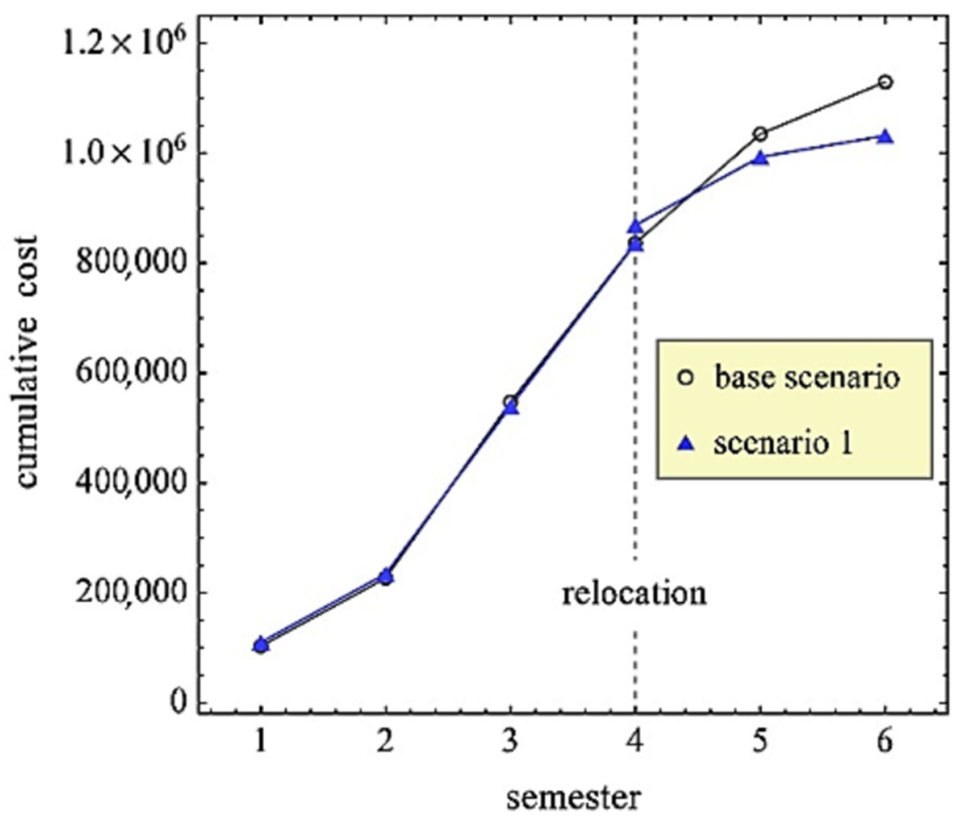
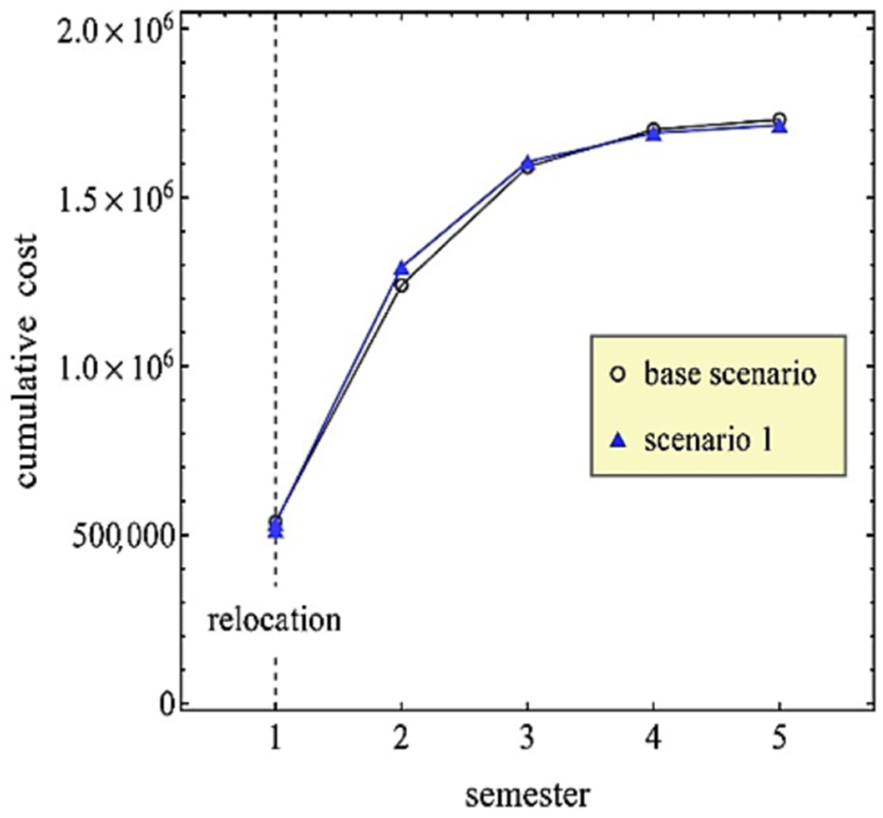
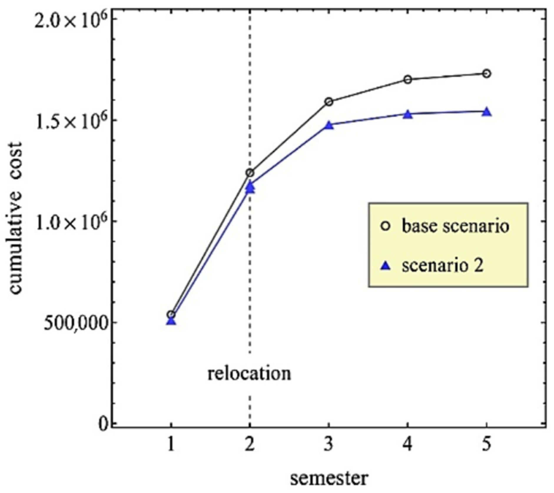
The total duration of the project was 3 years (6 semesters) and the chainages were from 8 + 550 to 23 + 350. The number of available locations that could host the construction site was nine, taking into account all the decision variables (Section 2.1). The total cost for the “ideal” location (i = 14 + 850) of construction site, without relocation (base scenario), was calculated as 1,129,475.59 €. In this case, following the execution methodology chosen by the constructor, the “ideal scenario” results in one relocation of the construction site (i1 = 14 + 650 for 1st to 4th semester, i2 = 19 + 450 for 5th to 6th semester) and the total savings are 97,759.69 €. The relocation for this scenario should take place at the end of the 4th semester. Table 6 summarizes some of the scenarios investigated. Figure 4, Figure 5 and Figure 6 graphically present cash flows between different scenarios.
After the relocation of the site, the total operating costs begin to fall and that conclusion is in line with the construction schedule which includes the main tasks to be executed at the last part of the project.
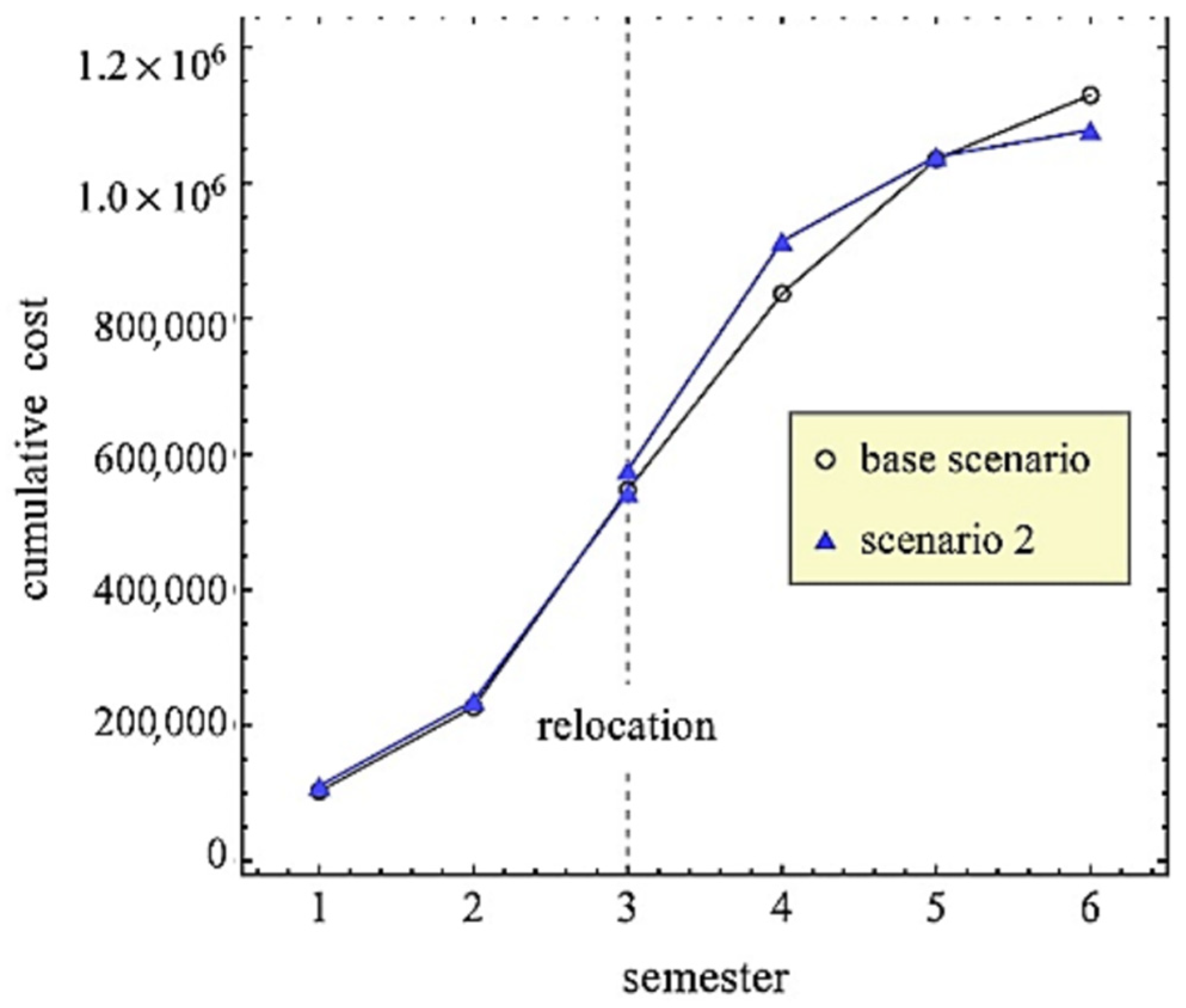
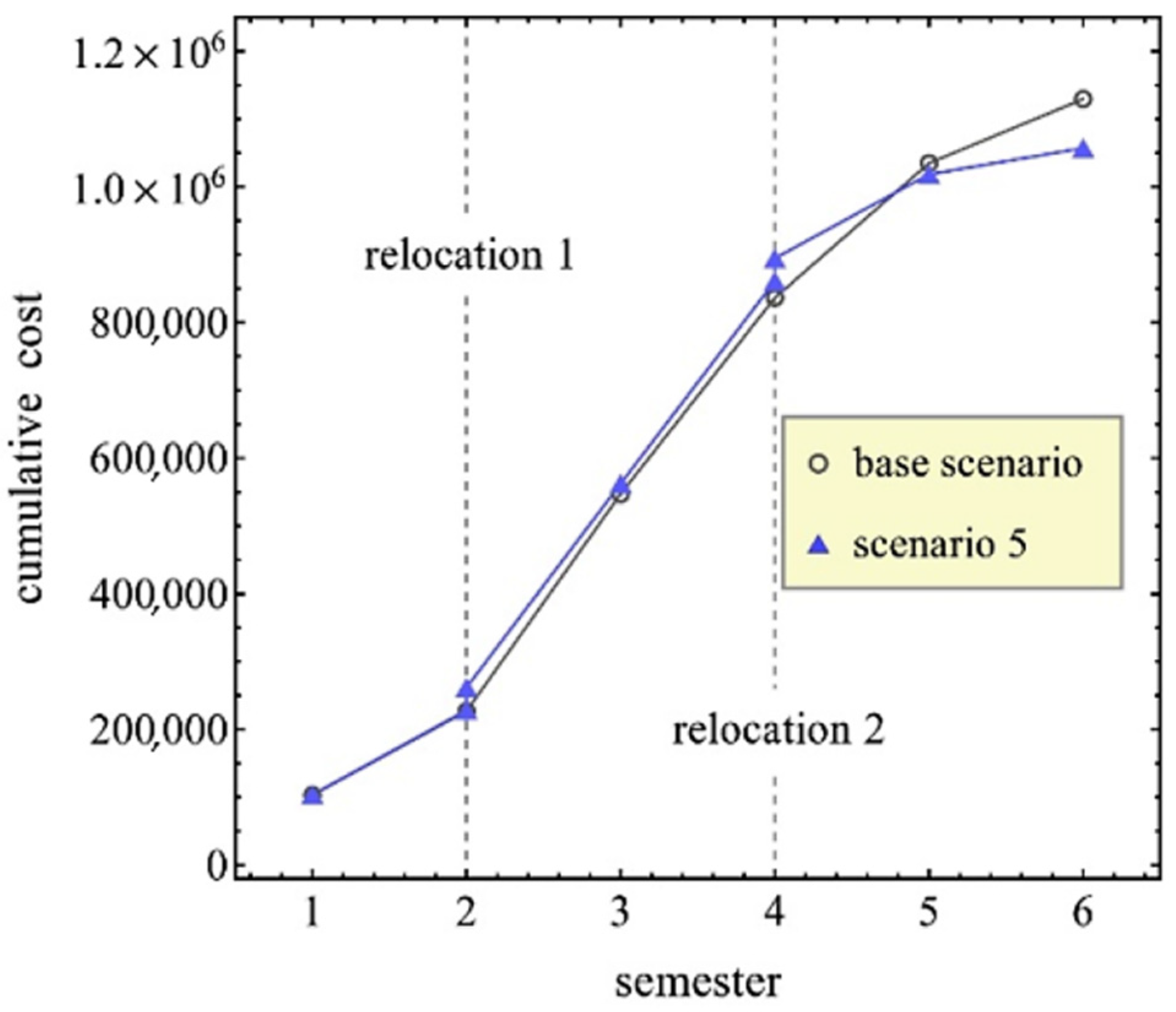
Sensitivity analysis 1: The division of the whole project into two parts was examined, the first part from chainage 8 + 550 to chainage 15 + 550 and the second part from chainage 15 + 650 to chainage 23 + 350. Table 7 presents two scenarios of this case. In Scenario 1, after the completion of the first part, and the relocation of the construction site, the work on the second part starts. In Scenario 2, the execution of the earthworks and the relative technical works are performed at the first part of the project, the second stage involves the execution of the earthworks and the relative technical works at the second part of the project, and the third stage includes the execution of the asphalt pavement at the first and second part. These scenarios are compared with the base scenario Section 4.3/Case Study 2 with TC = 1,129,475.59 €. Scenario 1 creates a profit of 532,881.89 €.
Sensitivity analysis 2: In cases that the area between the chainages 15 + 000 to 23 + 350 was not appropriate for site location, then the “ideal” scenario would be without relocation of the construction site, and specifically, the construction site should be placed in chainage 14 + 850 (base scenario Section 4.3/Case Study 2) with no profit.
Sensitivity analysis 3: If we assume that there were no technical works, then Scenario 3 would be “ideal” with one relocation and a total profit of 92,094.71 € (Scenario 3 Section 4.3/Case study 2).
Sensitivity analysis 4: In case that the machines were stored at the construction site, the “ideal” scenario would be with one relocation at the end of the 3rd semester with (Scenario 2 Section 4.3/Case Study 2) a total profit of 144,844.95 €.
4.4. Analysis and Results of Case Study 3
The available locations to host the construction site are provided as an optimization of the accepted slopes and road networks. The construction site for this part of the road was 45.485 m2, and during the construction phase, it was established in the chainage 14 + 350 for the whole construction period.
According to the project data, for each location, the maximum number of machines and their exact number as used for each task are as follows:
- 1 excavator (with a bucket capacity of 2.41 m3)
- 1 loader (with a bucket capacity of 4.30 m3)
- 1 crane truck
- 6 earthmoving trucks
- 4 road trucks
- 4 asphalt trucks
- 1 pavers
- 1 finisher
- 1 water tank
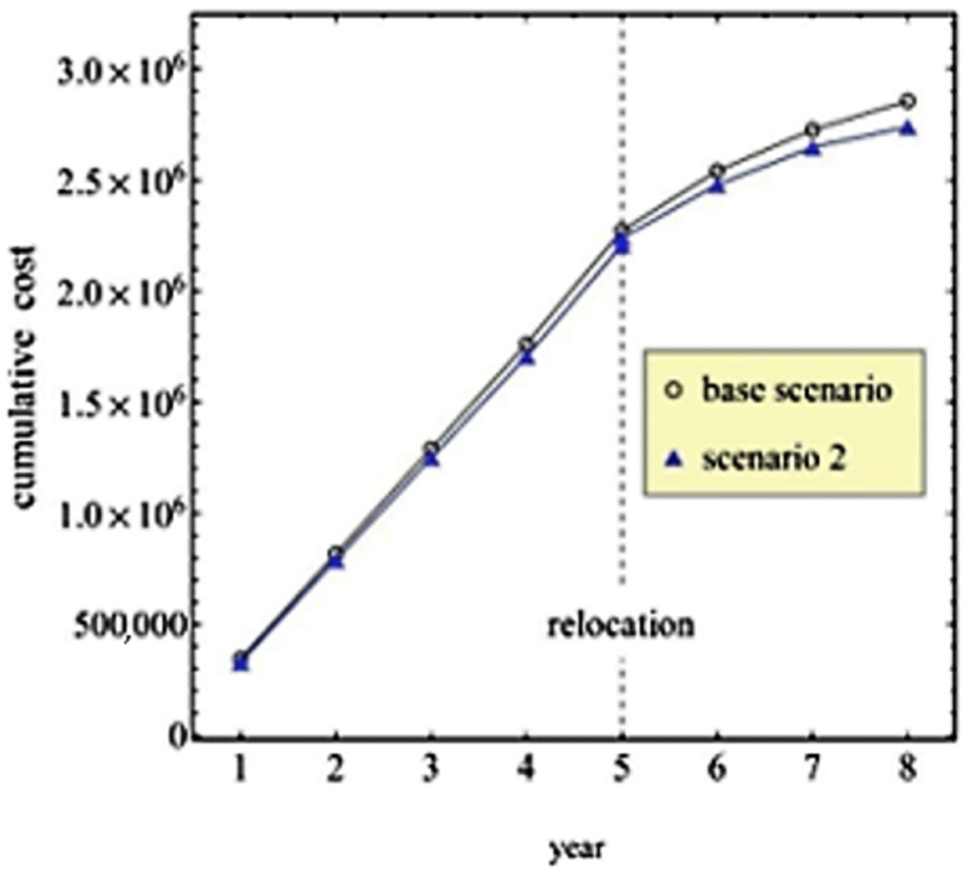
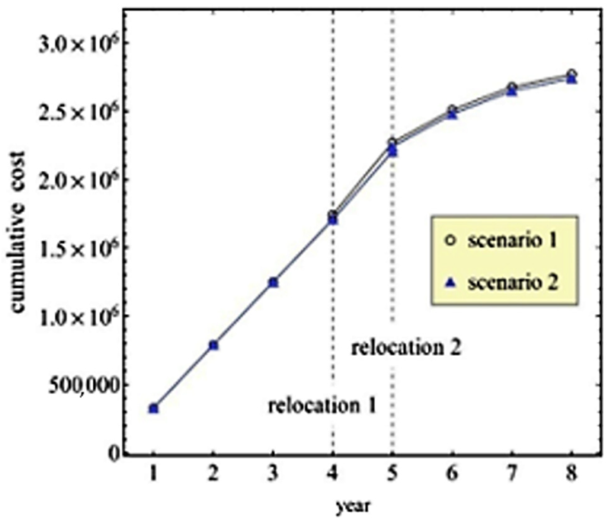
The excavator is for work on soil excavations; the loader is to load them; earthmoving trucks are for the transport of soils to the construction site or on other worksites such as embankment; road and asphalt trucks are for the transport of the above materials from the construction site to the workstation; the paver is for the condensation of the soils, base, background, and asphalt; the finisher is for the paving of asphalt and water tanks for the transport of water to the work site. The price of fuel was considered 1.10 €/L and the operator’s wage 80 €/day.The total cost for the “ideal” location (i = 14 + 050) without relocation (base scenario) is 2.857.596,34 €. For this case study, the “ideal” scenario with one relocation (i1 = 14 + 350, i2 = 11 + 350) creates a profit of 122,841.51 €. The relocation for this scenario should take place at the end of the 5th year of the construction. Table 8 presents some of the scenarios that were investigated.
Figure 7, Figure 8 and Figure 9 graphically present the cash flows of each scenario for Case Study 3.
Sensitivity analysis 1: The construction methodology examined includes the division of the whole project into two parts, the first part from chainage 00 + 000 to chainage 11 + 250, and the second part from chainage 12 + 350 to chainage 24 + 450. The three scenarios of this case are depicted in Table 9. In Scenario 1, after the completion of the first part and the relocation of the construction site, the works on the second part start. In Scenario 2, after the completion of the earthworks and technical works in the entire project and the relocation of the construction site, the execution of the asphalt pavement starts. For this scenario, almost no profit is earned (3057.16 €). In Scenario 3, earthworks and technical works are executed in the first part of the project, and then these works are executed in the second part. It follows the asphalt pavement of the whole project. These scenarios are compared with the base scenario Section 4.4/Case Study 3 with TC 2,857,596.34 €. Scenario 1 creates a profit of 1,336,869.89 €, and Scenario 3 generates a profit of 1,048,440.31 €.
Sensitivity analysis 2: If the project was not included the technical works and their work quantities, the initial cost of no relocation scenario would be 2.783.911,79 € (base scenario Section 4.4/Case Study 3) and the total cost of the previous “ideal” scenario would now be 2.664.357,07 € (Scenario 2 Section 4.4/Case Study 3). For this hypothesis, no profit is gained.
4.5. Analysis and Results of Case Study 4
The scope of the project was the construction of the remaining work for the completion of the contract “Construction of road connection of the Aktio Region with the Western Axis North-South”. It is a motorway with two (2) lanes of traffic per direction with a total width of 3.5 m each, with a total width divider of 2.00 m and an Emergency Lane 0.50 m wide in each direction. The criteria for the existing road network and acceptable ground gradients are met, so it was considered that all locations were available to accommodate the site. The operation of the site was as follows. (a) Excavation products were divided into suitable and unsuitable. The appropriate earthworks were driven directly to the embankments. (b) The supply of material for the construction site was carried out by the construction site. (c) The way in which plant land was managed is equivalent to earthmoving. (d) Aggregates used for the subbase and base of road were stored in silos at the construction site and transported to the workstation by transport trucks. (e) Concrete and asphalt were produced on-site and were transported to project by transport trucks. (f) All trucks and tankers were stored on the construction site, while excavators, pavers and asphalt machinery were left at the project. (g) Finally, the refueling of excavators, pavers, and asphalt machines was carried out by tankers.
According to the project data, for each location, the maximum number of machines and their exact number, as used for each task, were as follows:
- 2 excavators (with a bucket capacity of 1.32 m3)
- 2 loaders (with a bucket capacity of 2.45 m3)
- 10 earthmoving trucks
- 8 road trucks
- 5 asphalt trucks
- 8 pavers
- 1 finisher
- 4 water tanks
Excavators work on soil excavations; loaders load them; earthmoving trucks are for the transport of soils to the construction site; road and asphalt trucks are for the transport of the above materials from the construction site to the workstation; the paver was for the condensation of the soils, base, background and asphalt; the finisher was for the paving of asphalt; and water tanks were for the transport of water to the work site. The price of fuel was considered 1.098 €/L and the operator’s wage 80 €/day.
The quantities of each section of road were separated by 100 m for the whole project, and then the work for the five semesters was determined separately (1st, 2nd, 3rd, 4th, 5th) and for any possible combination of consecutive semesters (e.g., 1st–2nd, 3rd–4th–5th, 2nd–3rd–4th, etc.). The cost equation includes both the cost of fuel and the cost of truck and tank operators.
The cost-minimizing position is where the total movements of trucks and tanks are shared. The “ideal” position for the whole project was calculated at 29 + 100 chainage with a total cost of TC = 1,730,958.54 €. Following the same procedure, the “ideal” positions were calculated for each semester separately. The possibility of one or more relocations of the site was investigated. Based on the combinations of semesters and transportation costs, the different scenarios were examined with their respective total costs and profits.
For this project, the “ideal” locations are the installation of the site at 32 + 200 until the end of the second semester (12/2019) and then relocation of the site at 24 + 900 until the end of the project (6/2021). Following this procedure, the profit for the contractor is about 186,000 €. The results of some scenarios are presented in Table 10.
Figure 10, Figure 11 and Figure 12 graphically present the cash flows of each scenario for Case Study 4.
Sensitivity analysis 1: The construction methodology splits the project into two parts, the first part from chainage 17 + 700 to chainage 33 + 100 and the second part from chainage 33 + 200 to chainage 48 + 500. Thus, a site relocation is needed after the completion of the first part. The resulting cost is compared with the total cost for the “ideal” location (i = 29 + 100) of construction site without relocation (TC = 1,730,958.54 €); a profit of 57,061.17 € (Table 11) is accrued. That profit accounts almost for 3.3% of the total cost of the construction site and for 0.11% of the total cost of the project (TC = 54,000,000 €).
Sensitivity analysis 2: If the price of fuel was 9% lower (from 1.098 €/L to 1.00 €/L), the total cost of the project without relocation of the site would be 1,612,380.98 €. This would create a profit of 118,577,17 €. That profit accounts for almost 6.9% of the total cost of the construction site and for 0.22% of the total cost of the project (TC = 54,000,000 €).
5. Discussions
The advantage of dynamic planning of construction site is that it provides the constructor with a significant reduction in the operating costs of the construction site, especially in large-scale linear projects with profit that could cover its financial expenses, as happens in Case Studies 2, 3, and 4. The “ideal” scenario in Case Study 3 is the one with one relocation in the 5th year. From this relocation, the profit for the contractor escalates to 122,841.51 €. This amount could cover financing costs and provide better cash flows for the contractor. In Case Study 4, the profit is even greater, and it rises to 186,402.49 €. A sensitivity analysis was also performed in order to investigate the extent by combining different construction methodologies and taking into account macroeconomic factors. It was found that the selection of different construction methodologies could remarkably raise the profit and reach even 1% of the total budget. If different approaches in time sequence of activities are adopted, then the profit increases remarkably and can reach 1.5% of the budget, as happens in Case Study 4. The proposed approach of site relocation does not provide the same results for small linear projects, as is derived in Case Study 1. Once the schedule of project is confirmed and the volume mass diagram (Bruckner) is finalized, then the proposed algorithm (Figure 3) can be performed. Future research could examine the impact of the possible relocations on project’s time schedule.
6. Concluding Remarks
The nature of dynamic construction site planning requires the development and implementation of optimization processes that consider the dynamic interdependencies among location decisions of construction sites in different project phases. This paper presents the development and evaluation of an optimizing model of dynamic planning of construction site that deals with the problem of site location in a comprehensive and multifaceted way, being a useful decision tool in the hands of project managers. The algorithm indicates the “ideal” location where the cost of the transportation of the machinery, the unproductive time due to workers transportations, and finally the costs related to road network rehabilitation are minimized for each scenario investigated; then, it calculates the possible relocation of the construction site in relation to the advancement rate of the project to examine the best scenario that minimizes overall cost during the construction period. The proposed model was applied in four real case studies, and it was found to be a powerful optimization tool capable of producing cost-effective solutions derived from the dynamic relocation of construction sites for linear projects. The profits that the application of the proposed model creates could cover the financial costs of the contractor, which is a very important issue for the liquidity and thus the economic viability of such projects.
Author Contributions
Conceptualization, K.P. and N.A.; methodology, K.P., N.A., A.Z., and A.N.; software, A.Z. and A.N.; supervision, K.P.; validation, N.A., A.Z., and A.N.; writing—original draft preparation, K.P., N.A., A.Z., and A.N.; writing—review and editing, K.P. All authors have read and agreed to the published version of the manuscript.
Funding
This research received no external funding.
Data Availability Statement
The data presented in this study are available on request from the corresponding author. The data are not publicly available due to cost sensitive reasons.
Acknowledgments
This research would not have been possible without the valuable contribution of the project managers, site managers, and superintendents of the projects analyzed. In addition, the authors would like to thank the anonymous site engineers who with their comments helped to enhance the content of this study.
Conflicts of Interest
The authors declare no conflict of interest.
References
- Papadaki, I.; Chassiakos, A. Multi-objective construction site layout planning using genetic algorithms. Procedia Eng. 2016, 164, 20–27. [Google Scholar] [CrossRef]
- Elbeltagi, E.; Hosny, A.; Eldosouky, A. Schedule-dependent evolution of site layout planning. Constr. Manag. Econ. 2001, 19, 689–697. [Google Scholar] [CrossRef]
- Ning, X.; Lam, K.C.; Lam, M.C.K. A decision-making system for construction site layout planning. Autom. Constr. 2011, 20, 459–473. [Google Scholar] [CrossRef]
- Heesom, D.; Mahdjoubi, L.; Proverbs, D. A dynamic VR system for visualizing construction space usage. In Construction Research Congress; American Society of Civil Engineers: Reston, VA, USA, 2003. [Google Scholar]
- Chau, K.; Anson, M.; Zhang, J. 4D dynamic construction management and visualization software: 1. Development. Autom. Constr. 2005, 14, 512–524. [Google Scholar] [CrossRef] [Green Version]
- Chavada, R.; Dawood, N.; Kassem, M. Construction Workspace Management: The Development and Application of a Novel nD Planning Approach and Tool. J. Inf. Technol. Constr. 2012, 17, 213–236. [Google Scholar]
- Ma, Z.; Shen, Q.; Zhang, J. Application of 4D for dynamic site layout and management of construction projects. Autom. Constr. 2005, 14, 369–381. [Google Scholar] [CrossRef]
- Li, H.; Love, P.E.D. Genetic search for solving construction site-level unequal-area facility layout problems. Autom. Constr. 2000, 9, 217–226. [Google Scholar] [CrossRef]
- Huang, C.; Wong, C.K. Optimisation of site layout planning for multiple construction stages with safety considerations and requirements. Autom. Constr. 2015, 53, 58–68. [Google Scholar] [CrossRef]
- Chau, K.W. A two-stage dynamic model on allocation of construction facilities with genetic algorithm. Autom. Constr. 2004, 13, 481–490. [Google Scholar] [CrossRef]
- Osman, H.M.; Georgy, M.E.; Ibrahim, M.E. A hybrid CAD-based construction site layout planning system using genetic algorithms. Autom. Constr. 2003, 12, 749–764. [Google Scholar] [CrossRef]
- Alavipour, R.; Arditi, D. Optimizing Financing Cost in Construction Projects with Fixed Project Duration. J. Constr. Eng. Manag. 2018, 144, 04018012. [Google Scholar] [CrossRef]
- Omopariola, E.; Windapo, A.; Edwards, D.; Twala, W. Contractors’ perceptions of the effects of cach flow on construction projects. J. Eng. Des. Technol. 2019. [Google Scholar] [CrossRef]
- Tijssen, R.J.; Van Raan, A.F. Mapping Changes in Science and Technology: Bibliometric Co-Occurrence Analysis of the R&D Literature. Eval. Rev. 1994, 18, 98–115. [Google Scholar] [CrossRef]
- Cobo, M.J.; López-Herrera, A.G.; Herrera-Viedma, E.; Herrera, F. Science mapping software tools: Review, analysis, and cooperative study among tools. J. Am. Soc. Inf. Sci. Technol. 2001, 62, 1382–1402. [Google Scholar] [CrossRef]
- van Eck, N.J.; Waltman, L. Software survey: VOSviewer, a computer program for bibliometric mapping. Scientometrics 2010, 84, 523–538. [Google Scholar] [CrossRef] [Green Version]
- van Eck, N.J.; Waltman, L. Text Mining and Visualization Using VOSviewer. 2011. Available online: http://www.vosviewer.com (accessed on 31 March 2020).
- van Eck, N.J.; Waltman, L. Visualizing Bibliometric Networks. Meas. Sch. Impact 2014, 285–320. [Google Scholar] [CrossRef]
- Zouein, P.P.; Tommelein, I.D. Dynamic Layout Planning Using a Hybrid Incremental Solution Method. J. Constr. Eng. Manag. 1998, 125, 400–408. [Google Scholar] [CrossRef] [Green Version]
- Said, H.; El-Rayes, K. Optimizing the planning of construction site security for critical infrastructure projects. Autom. Constr. 2010, 19, 221–234. [Google Scholar] [CrossRef]
- Cheng, M.-Y.; Yang, S.-C. GIS-Based Cost Estimates Integrating with Material Layout Planning. J. Constr. Eng. Manag. 2001, 127. [Google Scholar] [CrossRef]
- Elbeltagi, E.; Hegazy, T.; Eldosouky, A. Dynamic Layout of Construction Temporary Facilities Considering Safety. J. Constr. Eng. Manag. 2004, 130, 534–541. [Google Scholar] [CrossRef]
- Xu, J.; Li, Z. Multi-Objective Dynamic Construction Site Layout Planning in Fuzzy Random Environment. Autom. Constr. 2012, 27, 155–169. [Google Scholar] [CrossRef]
- Andayesh, M.; Sadeghpour, F. Dynamic site layout planning through minimization of total potential energy. Autom. Constr. 2013, 31, 92–102. [Google Scholar] [CrossRef]
- Said, H.; El-Rayes, K. Performance of global optimization models for dynamic site layout planning of construction projects. Autom. Constr. 2013, 36, 71–78. [Google Scholar] [CrossRef]
- Tam, C.; Tong, T.; Leung, A.; Chiu, G. Site layout planning using nonstructural fuzzy decision support system. J. Constr. Eng. Manag. 2002, 128, 220–231. [Google Scholar] [CrossRef] [Green Version]
- Li, H.; Love, P. Site-level facilities layout using genetic algorithms. J. Comput. Civ. Eng. 1998, 12, 227–231. [Google Scholar] [CrossRef]
- Yeh, I.-C. Construction-site layout using annealed neural network. J. Comput. Civ. Eng. 1995, 9, 201–208. [Google Scholar] [CrossRef]
- Cheng, J.C.P.; Kumar, S.S. A BIM based construction site layout planning framework considering actual travel paths. In Proceedings of the 31st International Symposium on Automation and Robotics in Construction and Mining, ISARC 2014, Sydney, Australia, 9–11 July 2014; pp. 450–457. [Google Scholar] [CrossRef] [Green Version]
- Al Hawarneh, A.; Bendak, S.; Ghanim, F. Dynamic facilities planning model for large scale construction projects. Autom. Constr. 2019, 98, 72–89. [Google Scholar] [CrossRef]
- Zolfagharian, S.; Irizarry, J. Current Trends in Construction Site Layout Planning. In Proceedings of the Construction Research Congress, Atlanta, GA, USA, 19–21 May 2014; pp. 1723–1732. [Google Scholar]
- Greek Government. Building Regulation of Greece; Article 21; Greek Parliament: Athens, Greece, 1989. [Google Scholar]
- Lagro, J. Site Analysis: A Contextual Approach to Sustainable Land Planning and Site Design, 2nd ed.; John Wiley & Sons, Inc.: Hoboken, NJ, USA, 2007. [Google Scholar]
- Peurifoy, R.; Schexnayder, C.; Shapira, A.; Schimitt, R. Contruction Planning, Equipment, and Methods, 8th ed.; McGraw Hill International Edition: New York, NY, USA, 2001. [Google Scholar]
- Petroutsatou, K.; Marinelli, M. Construction Equipment, Operational Analysis and Economics of Civil Engineering Projects, 2nd ed.; KRITIKI SA: Athens, Greece, 2018. [Google Scholar]
- Razavialavi, S.; Abourizk, S.; Alanjari, P. Estimating the Size of Temporary Facilities in Construction Site Layout Planning Using Simulation. In Proceedings of the Construction Research Congress, Atlanta, GA, USA, 19–21 May 2014; pp. 70–79. [Google Scholar]
- Lee, K.H.A. Optimization of Construction Site Layout Planning by Generic Algorithm. Doctoral Dissertation, City University of Hong Kong, Hong Kong, August 2013. [Google Scholar]
- Sanad, H.; Ammar, M.; Ibrahim, M. Optimal Construction Site Layout Considering Safety and Environmental Aspects. J. Constr. Eng. Manag. 2008, 134, 536–544. [Google Scholar] [CrossRef]
- Marinelli, M.; Lambropoulos, S.; Petroutsatou, K. Earthmoving trucks condition level prediction using neural networks. J. Qual. Maint. Eng. 2014, 20, 182–192. [Google Scholar] [CrossRef]
Figure 1.
Main steps of the txt mining process using VosViewer.

Figure 2.
Visualized map of network.

Figure 3.
Optimization algorithm.

Scheme 1.
Map of the second case study project.

Scheme 2.
Map of the third and fourth case study project.

Figure 4.
Comparison of cumulative costs.

Figure 5.
Comparison of cumulative costs.

Figure 6.
Comparison of cumulative costs between scenarios.

Figure 7.
Comparison of cumulative costs.

Figure 8.
Comparison of cumulative costs.

Figure 9.
Comparison of cumulative costs between scenarios.

Figure 10.
Comparison of cumulative costs between scenarios.

Figure 11.
Comparison of cumulative costs between scenarios.

Figure 12.
Comparison of cumulative costs between scenarios.


Table 1.
Word Occurrences in Clusters.
| Cluster 1 | Cluster 2 | Cluster 3 |
|---|---|---|
| Construction Site Layout | Construction project | Construction |
| Algorithm | Dynamic site layout planning | BIM |
| Genetic Algorithm | Effectiveness | Cost |
| Location | Model | |
| Safety | Time | |
| Space | ||
| Temporary Facility |
Table 2.
Work quantities for chainage 18 + 450.
| Quantities (m3) | ||||||||||
|---|---|---|---|---|---|---|---|---|---|---|
| Chainage | Embankment | Excavations | Drain Age | Plant Land | Sub Base | Base | Asphalt | Concrete | Rebars | Drain Pipes (kgr) |
| 18 + 450 | 1847.4 | 20,561.54 | 308.22 | 2409.6 | 120 | 230 | 10,230 | 44 | 0 | 504,000 |
Table 3.
Required movements for chainage 18 + 450.
| Number of Transportation Trucks | |||||||||
|---|---|---|---|---|---|---|---|---|---|
| Chainage | Earthmoving Trucks | Drain Age | Subbase | Base | Asphalt | Concrete | Rebars | Drainpipes | Tanks |
| 18 + 450 | 480 | 46 | 18 | 34 | 620 | 30 | 0 | 48 | 76 |
Table 4.
Optimization process for dynamic planning of construction site.
| Scenario X | Location | Cost |
|---|---|---|
| 1st + 2nd + … + N | A | A € |
| (Ν + 1) + … + Last | B | B € |
| Relocation cost | R € | |
| Total scenario cost | (A + B+R+ user’s target) = Χ € | |
| Profit | (TC(i) − X) = Υ € |
Table 5.
Operating costs results of the first project.
| Scenarios | Period | Ideal Location | Operating Cost | Relocation Cost | Total Cost | Profit/Loss |
|---|---|---|---|---|---|---|
| Base Scenario without Relocation | 1st to 6th | 1 + 550 | 142,044.10 € | 142,044.10 € | 37,536.73 € | |
| Ideal = 2 + 650 | 104,507.36 € | 104,507.36 € | ||||
| 3 + 550 | 122,580.05 € | 122,580.05 € | 18,072.68 € | |||
| 1 | 1st to 3rd | Ideal = 3 + 050 | 39,127.72 € | 24,500.00 € | 147,232.24 € | 42,724.87 € |
| 4th to 6th | Ideal = 2 + 050 | 83,604.51 € | ||||
| 2 | 1st to 4th | Ideal = 3 + 050 | 95,602.17 € | 24,500.00 € | 168,100.25 € | 63,592.88 € |
| 5th to 6th | Ideal = 2 + 050 | 47,998.08 € | ||||
| 3 | 1st to 2nd | Ideal = 4 + 250 | 4555.69 € | 49,000.00 € | 158,327.29 € | 53,819.92 € |
| 3rd to 4th | Ideal = 2 + 950 | 56,773.51 € | ||||
| 5th to 6th | Ideal = 2 + 050 | 47,998.08 € |
Table 6.
Operating costs results of the second project.
| Scenarios | Period | Ideal Location | Operating Cost | Relocation Cost | Total Cost | Profit/Loss |
|---|---|---|---|---|---|---|
| Base scenario without relocation | 1st to 6th | 11 + 650 | 1.469,784.12 € | 1,469,784.12 € | 340,308.53 € | |
| 11 + 850 | 1,436,149.95 € | 1,436,149.95 € | 306,674.36 € | |||
| 14 + 050 | 1,166,642.71 € | 1,166,642.71 € | 37,167.12 € | |||
| Ideal = 14 + 850 | 1,129,475.59 € | 1,129,475.59 € | ||||
| 19 + 450 | 1,363,944.17 € | 1,363,944.17 € | 234,468.58 € | |||
| 1 | 1st to 4th | Ideal = 14 + 650 | 835,489.50 € | 33,500.00 € | 1,031,715.90 € | 97,759.69 € |
| 5th to 6th | Ideal = 19 + 450 | 162,726.40 € | ||||
| 2 | 1st to 3rd | Ideal = 14 + 050 | 538,520.79 € | 33,500.00 € | 1,077,709.39 € | 51,766.20 € |
| 4th to 6th | Ideal = 19 + 450 | 505,688.60 € | ||||
| 3 | 1st to 2nd | Ideal = 14 + 850 | 227,522.67 € | 67,000.00 € | 1,089,889.16 € | 39,586.43 € |
| 3rd | Ideal = 11850 | 289,677.88 € | ||||
| 4th to 6th | Ideal = 19450 | 505,688.60 € | ||||
| 4 | 1st | Ideal = 14850 | 103,764.33 € | 67,000.00 € | 1,060,204.67 € | 69,270.93 € |
| 2nd to 4th | Ideal = 14250 | 726,713.93 € | ||||
| 5th to 6th | Ideal =1 9450 | 162,726.40 € | ||||
| 5 | 1st to 2nd | Ideal = 14850 | 227,522.67 € | 67,000.00 € | 1,057,209.26 € | 72,266.33 € |
| 3rd to 4th | Ideal = 14050 | 599,960.19 € | ||||
| 5th to 6th | Ideal = 19450 | 162,726.40 € |
Table 7.
Profit gained in case of changing sequence of works.
| Scenario | Relocation | Chainage | Ideal Location | Operating Cost | Relocation Cost | Total Cost | Profit/Loss |
|---|---|---|---|---|---|---|---|
| 1 | 1 | 8550–15,550 | Ideal = 11,850 | 258,293.48 € | 33,500.00 € | 596,593.71 € | 532,881.89 € |
| 15,650–23,350 | Ideal = 19,450 | 304,800.23 € | |||||
| 2 | 2 | 8550–15,550 (Earthworks and technical works) | Ideal = 11,850 | 157,274.60 € | 67,000.00 € | 864,536.16 € | 264,939.43 € |
| 15,650–23,350 (Earthworks and technical works) | Ideal = 19,450 | 177,154.92 € | |||||
| 8550–23,550 (Asphalt paving) | Ideal = 14,850 | 463,106.64 € |
Table 8.
Operating costs results of the third project.
| Scenarios | Period | Ideal Location | Operating Cost | Relocation Cost | Total Cost | Profit/Loss |
|---|---|---|---|---|---|---|
| Base scenario (without relocation) | 1st to 8th | 2250 | 5,763,803.74 € | € | 5,763,803.74 € | 2,899,958.93 € |
| 11,850 | 4,619,248.26 € | € | 4,619,248.26 € | 1,755,403.45 € | ||
| Ideal = 14,050 | 2,857,596.34 € | € | 2,857,596.34 € | € | ||
| 19,450 | 4,191,612.89 € | € | 4,191,612.89 € | 1,334,016.54 € | ||
| 1 | 1st to 4th | Ideal = 14,350 | 1,706,998.63 € | 35,000.00 € | 2,769,518.63 € | 94,326.17 € |
| 5th to 8th | Ideal = 11,350 | 1,027,520 € | ||||
| 2 | 1st to 5th | Ideal = 14,350 | 2,203,460.65 € | 35,000.00 € | 2,741,003.30 € | 122,841.51 € |
| 3 | 6th to 8th | Ideal = 11,350 | 502,542.65 € | 35,000.00 € | 2,776,349.12 € | 85,234.69 € |
| 1st to 5th | Ideal = 14,350 | 2,203,460.65 € | ||||
| 6th to 7th | Ideal = 11,350 | 408.105,39 € | ||||
| 8th | Ideal = 9250 | 94.783,08 € |
Table 9.
Profit gained in operating costs by changing the construction method in the third project.
| Scenarios | Relocation | Chainage | Ideal Location | Operating Cost | Relocation Cost | Total Cost | Profit/Loss |
|---|---|---|---|---|---|---|---|
| 1 | 1 | 00 + 000–12 + 250 | Ideal = 4 + 650 | 753,963.36 € | 35,000.00 € | 1,526,975 € | 1,336,869.8 € |
| 12 + 350–24 + 450 | Ideal = 16 + 350 | 738,011.55 € | |||||
| 2 | 1 | 00 + 000–24 + 450(Earthworks and technical works) | Ideal = 14 + 350 | 2,230,291 € | 35,000.00 € | 2,860,788 € | 3057.16 € |
| 00 + 000–24 + 450 (Asphalt paving) | Ideal = 11 + 350 | 595,496.63 € | |||||
| 3 | 2 | 00 + 000–11 + 250 (Earthworks and technical works) | Ideal = 4 + 650 | 525,132.36 € | 70,000.00 € | 1,815,405 € | 1,048,440 € |
| 11 + 350–24 + 450 (Earthworks and technical works) | Ideal = 16 + 350 | 624,775.49 € | |||||
| 00 + 000–24 + 450 (Asphalt paving) | Ideal = 11 + 350 | 595,496.63 € |
Table 10.
Operating costs results of the fourth project.
| Scenarios | Period | Ideal Location | Operating Cost | Relocation | Total Cost | Profit/Loss |
|---|---|---|---|---|---|---|
| base scenario without relocation | 1st to 5th | Ideal = 29 + 100 | 1,730,958.54 € | € | 1,730,958.54 € | |
| 1 | 1st | Ideal = 31 + 600 | 514,192.94 € | 20,500 € | 1,714,344.73 € | 16,613.80 € |
| 2nd to 5th | Ideal = 27 + 500 | 1,179,651.79 € | ||||
| 2 | 1st to 2nd | Ideal = 32 + 200 | 1,160,901.17 € | 20,500 € | 1,544,556.05 € | 186,402.49 € |
| 3rd to 5th | Ideal = 24 + 900 | 363,154.88 € | ||||
| 3 | 1st to 3rd | Ideal = 30 + 200 | 1,576,311.55 € | 20,500 € | 1,645,045.46 € | 85,913.08 € |
| 4th to 5th | Ideal = 22 + 600 | 48,233.92 € |
Table 11.
Profit gained by splitting the project into two parts.
| Chainage | Site Location | Operating Cost | Relocation Cost | Total Cost | Profit/Loss |
|---|---|---|---|---|---|
| 17 + 700–33 + 100 | 25 + 300 | 603,613.73 € | 20,500.00 € | 1,673,897.37 € | 57,061.17 € |
| 33 + 200–48 + 500 | 44 + 500 | 1,049,783.64 € |
Publisher’s Note: MDPI stays neutral with regard to jurisdictional claims in published maps and institutional affiliations. |
© 2021 by the authors. Licensee MDPI, Basel, Switzerland. This article is an open access article distributed under the terms and conditions of the Creative Commons Attribution (CC BY) license (http://creativecommons.org/licenses/by/4.0/).
Share and Cite
MDPI and ACS Style
Petroutsatou, K.; Apostolidis, N.; Zarkada, A.; Ntokou, A. Dynamic Planning of Construction Site for Linear Projects. Infrastructures 2021, 6, 21. https://0-doi-org.brum.beds.ac.uk/10.3390/infrastructures6020021
AMA Style
Petroutsatou K, Apostolidis N, Zarkada A, Ntokou A. Dynamic Planning of Construction Site for Linear Projects. Infrastructures. 2021; 6(2):21. https://0-doi-org.brum.beds.ac.uk/10.3390/infrastructures6020021
Chicago/Turabian StylePetroutsatou, Kleopatra, Nikolaos Apostolidis, Athanasia Zarkada, and Aneta Ntokou. 2021. "Dynamic Planning of Construction Site for Linear Projects" Infrastructures 6, no. 2: 21. https://0-doi-org.brum.beds.ac.uk/10.3390/infrastructures6020021