Statistical Approach for Vibration-Based Damage Localization in Civil Infrastructures Using Smart Sensor Networks


Abstract
:
1. Introduction
- The possibility of onboard computation of the damage index at selected nodes, which autonomously and timely send alarm messages, without requiring complex transmission/synchronization strategies to convey data to a central processing unit.
- A limited wireless transmission rate thanks to the onboard computation of the damage index and the implementation of adaptive downsampling of the structural responses before transmission. The aim is to extract and transmit only the frequency bands containing the relevant information.
- The data-driven nature of the approach, which does not involve any model of the structure (either analytical or numerical, e.g., finite element models), thereby reducing the computational effort.
2. Instantaneous Identification of Modal Parameters
3. Damage Identification Method
3.1. The Damage Sensitive Feature: Interpolation Error
3.2. The Decentralized Algorithm: Clamped-Clump Interpolation Method
3.3. The Damage Index: Modified Statistical Interpolation Damage Index
4. Numerical Benchmark
4.1. Description of the Structure
4.2. Subsets of Sensors and Data Processing
4.3. Results
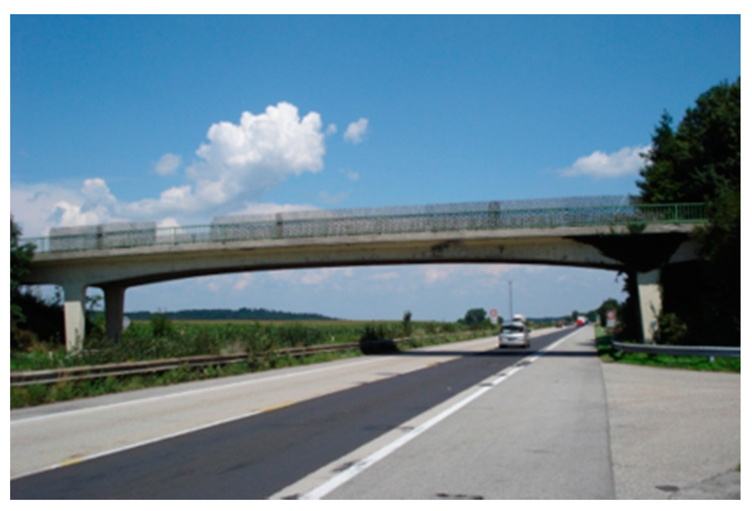
5. S101 Bridge
5.1. Description of the Bridge and Monitoring System
5.2. Subsets of Sensors and Data Processing
5.3. Results
6. Discussion
- (1)
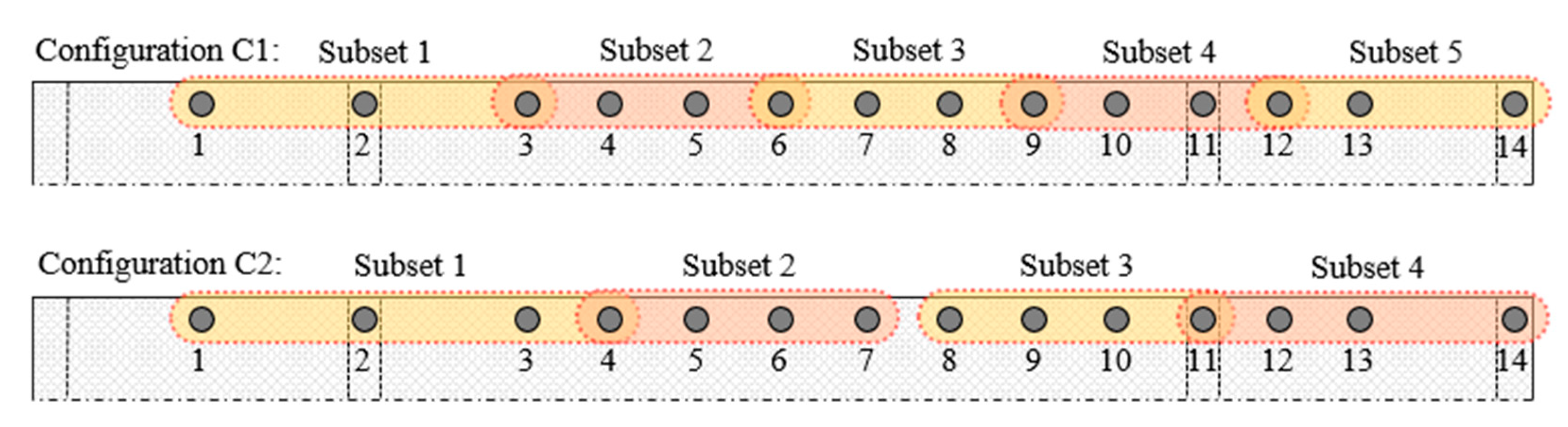
- Computation of instantaneous mode shapes using CFBs. The mode shapes are estimated using the responses over subsets of sensors organized according to different configurations.
- (2)
- Computation of instantaneous values of the damage feature, i.e., the interpolation error, at the inner sensors of each subset using the clamped-clump interpolation method.
- (3)
- Computation of a novel damage index, i.e., the MSIDI, from the statistical distributions of the interpolation error in the reference and the inspection state.
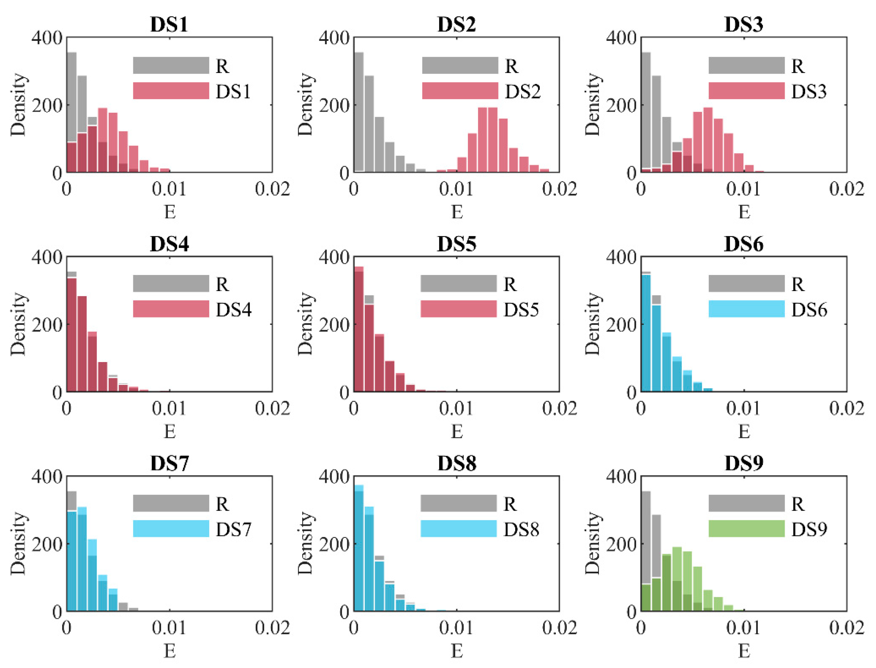
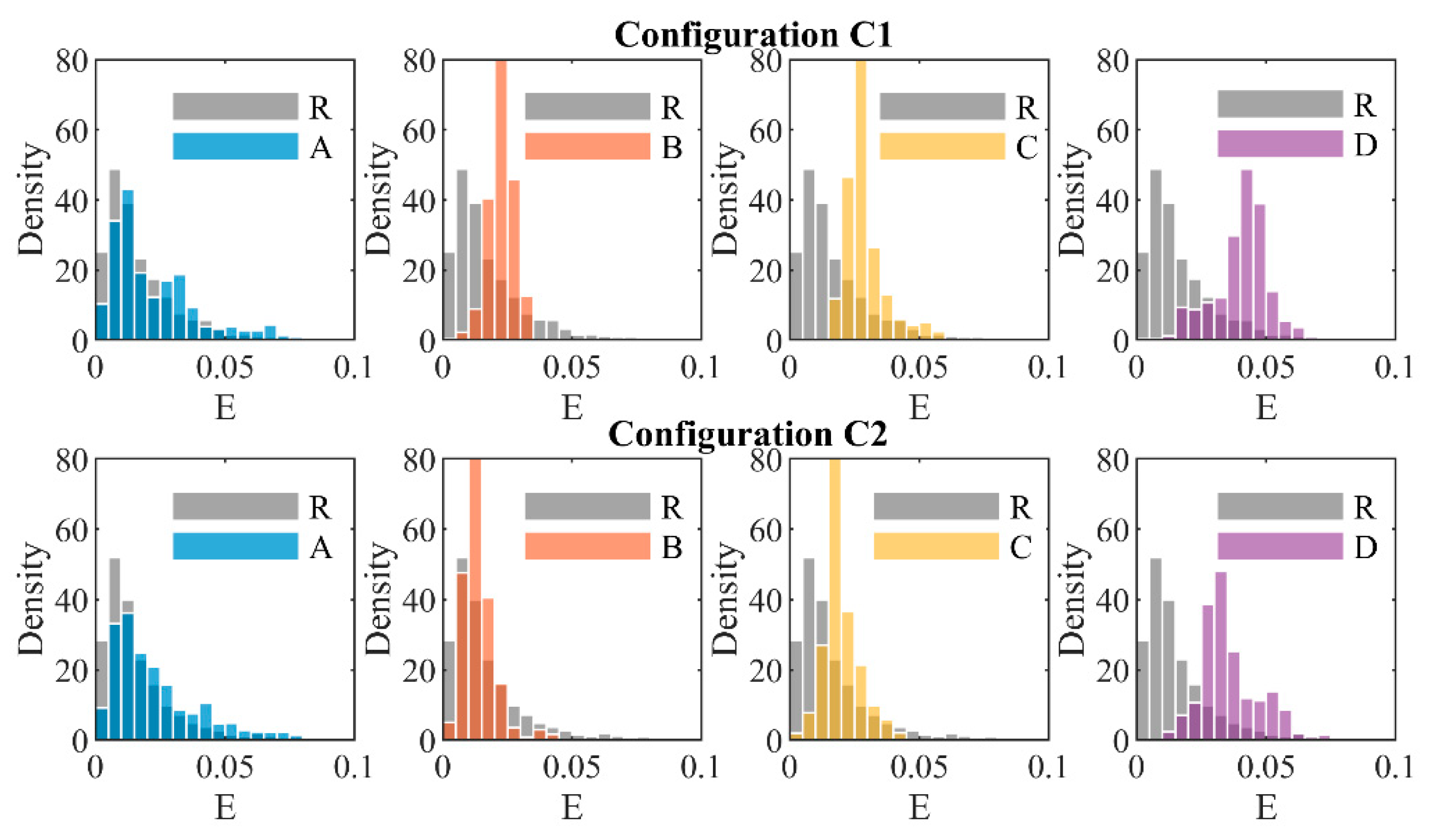
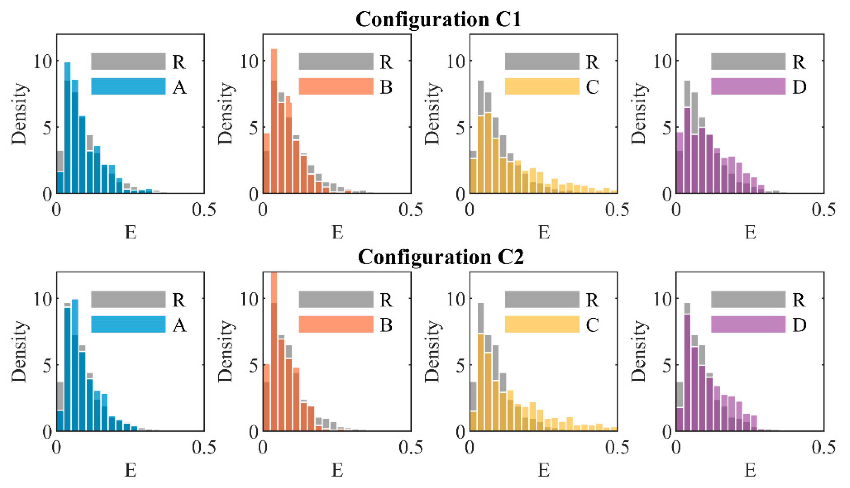
- In the damaged scenarios, the damage feature increases at the damage locations with respect to the reference condition. Conversely, the damage feature in the reference and the inspection state are similar at non-damaged locations. This is exemplified in Figure 5, Figure 10, and Figure 11, which display the histogram plot of the damage feature for different damage scenarios and at several sensor locations. It is noted, qualitatively, that the overlapping area between the distribution of the interpolation error in the reference and the damaged scenarios decreases as the magnitude of damage increases.
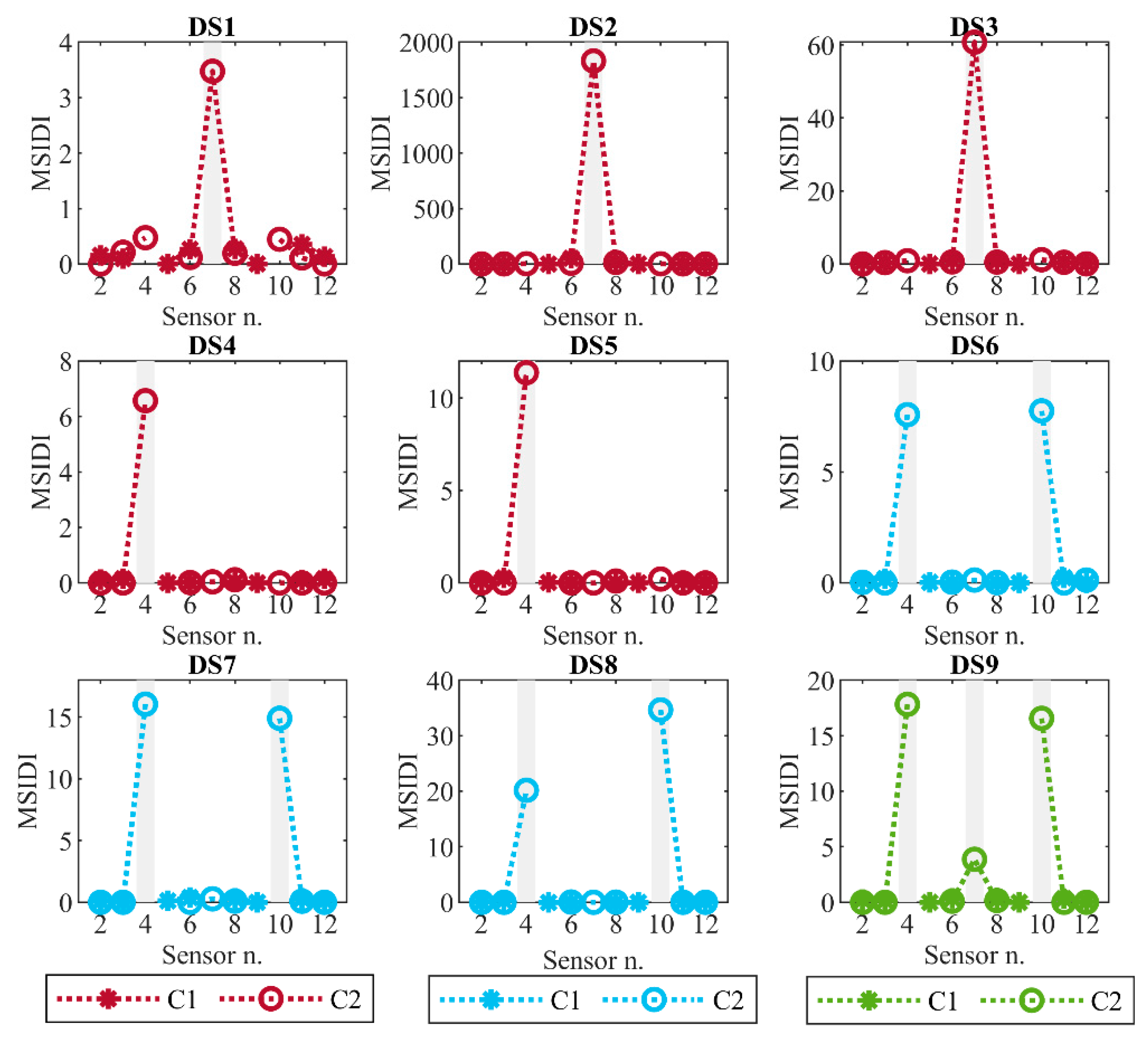
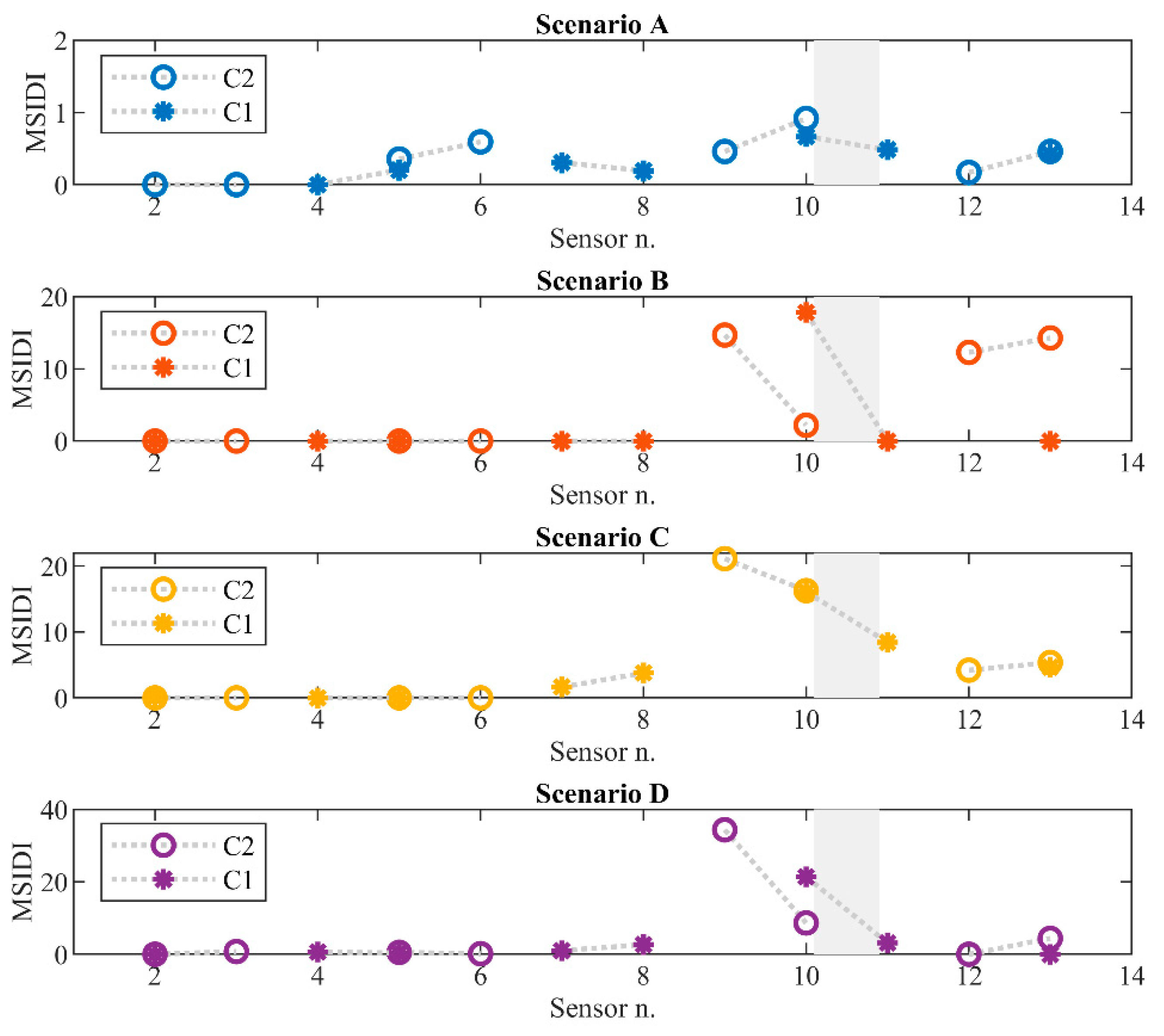
- For single damage scenarios, the values of the MSIDI in general increase according to the increasing severity of the damage. This is clearly shown by the comparison of DS1, DS3, and DS2 corresponding to increasing losses of stiffness at the same location (see the first row of Figure 6). This is directly linked to the definition of the damage indicator, see Equation (13).
- The same stiffness loss corresponds to different values of the damage index depending on the location of the damage. This is shown, for example, by the comparison of DS1 and DS4 or DS2 and DS5 corresponding to the same damage severity but different values of the damage feature.
- For multiple damage scenarios (e.g., DS9 in Figure 6), the detection of certain damages can be hindered by damages at other locations. This is not only due to the dependence of the damage index on the damage location (remarked at the previous point), but also on the dependence of the damage feature at a given location on damage at other locations. This is shown for example by the comparison between DS6 and DS9. In the second scenario, there is a further damaged section at midspan, but the value of the damage index at the central damage location is lower with respect to the others. This suggests that damage at midspan affects the values of the damage indexes at the other two locations.
- The comparison of the results obtained herein with those reported in Reference [28] using the SIDI show the higher sensitivity of the MSIDI with respect to the former version of the damage index.
- The threshold value used to compare the distribution of the interpolation error in the MSIDI is automatically determined, which simplifies the computation of the damage index.
- The evaluation of the damage features is carried out considering two different sensor subset configurations. This overcomes the difficulties related to the computation of the damage feature at the boundaries of the subsets.
7. Conclusions
Author Contributions
Funding
Data Availability Statement
Acknowledgments
Conflicts of Interest
References
- Limongelli, M.P.; Chatzi, E.; Döhler, M.; Lombaert, G.; Reynders, E. Towards extraction of vibration-based damage indicators. In Proceedings of the 8th European Workshop on Structural Health Monitoring, EWSHM 2016, Bilbao, Spain, 5–8 July 2016. [Google Scholar]
- Maeck, J.; Peeters, B.; De Roeck, G. Damage identification on the Z24 bridge using vibration monitoring. Smart Mater. Struct. 2001. [Google Scholar] [CrossRef]
- Pandey, A.K.; Biswas, M.; Samman, M.M. Damage detection from changes in curvature mode shapes. J. Sound Vib. 1991. [Google Scholar] [CrossRef]
- Stubbs, N.; Kim, J.T.; Topole, K.G. An efficient and robust algorithm for damage localization in offshore platforms. In Proceedings of the ASCE 10th Structures Congress, San Antonio, TX, USA, 13–15 April 1992; pp. 543–546. [Google Scholar]
- Limongelli, M.P. The interpolation damage detection method for frames under seismic excitation. J. Sound Vib. 2011. [Google Scholar] [CrossRef]
- Domaneschi, M.; Limongelli, M.P.; Martinelli, L. Damage detection in a suspension bridge model using the Interpolation Damage Detection Method. In Proceedings of the Sixth International Conference on Bridge Maintenance, Safety and Management, Stresa, Italy, 8–12 July 2012. [Google Scholar]
- Pozzi, M.; Der Kiureghian, A. Assessing the value of information for long-term structural health monitoring. In Proceedings of the SPIE 7984, Health Monitoring of Structural and Biological Systems 2011, San Diego, CA, USA, 7–10 March 2011; SPIE: Bellingham, DC, USA, 2011. [Google Scholar]
- Giordano, P.F.; Prendergast, L.J.; Limongelli, M.P. A framework for assessing the value of information for health monitoring of scoured bridges. J. Civ. Struct. Heal. Monit. 2020, 10, 485–496. [Google Scholar] [CrossRef]
- Giordano, P.F.; Limongelli, M.P. The value of structural health monitoring in seismic emergency management of bridges. Struct. Infrastruct. Eng. 2020, 1–17. [Google Scholar] [CrossRef]
- Celebi, M. Seismic Instrumentation of Buildings; U.S. Geological Survey Open-File Report 00-157, 37; U.S. Geological Survey: Menlo Park, CA, USA, 2000.
- Straser, E.G.; Kiremidjian, A.S.; Meng, T.H.; Redlefsen, L. Modular, wireless network platform for monitoring structures. In Proceedings of the International Modal Analysis Conference–IMAC, Santa Barabara, CA, USA, 2–5 February 1998. [Google Scholar]
- Watkins, D.S. Understanding the $QR$ Algorithm. SIAM Rev. 1982, 24, 427–440. [Google Scholar] [CrossRef]
- Golub, G.H.; Van Der Vorst, H.A. Eigenvalue computation in the 20th century. J. Comput. Appl. Math. 2000, 123, 35–65. [Google Scholar] [CrossRef] [Green Version]
- Cullum, J.K.; Willoughby, R.A. Lanczos Algorithms for Large Symmetric Eigenvalue Computations. Vol. I: Theory; SIAM: Philadelphia, PA, USA, 2002; Volume 41, ISBN 978-0-89871-523-1. [Google Scholar]
- Mucchielli, P.; Bhowmik, B.; Hazra, B.; Pakrashi, V. Higher-Order Stabilized Perturbation for Recursive Eigen-Decomposition Estimation. J. Vib. Acoust. Trans. ASME 2020, 142. [Google Scholar] [CrossRef]
- Bhowmik, B.; Tripura, T.; Hazra, B.; Pakrashi, V. Real time structural modal identification using recursive canonical correlation analysis and application towards online structural damage detection. J. Sound Vib. 2020. [Google Scholar] [CrossRef]
- Panda, S.; Tripura, T.; Hazra, B. First order error-adapted eigen perturbation for real-time modal identification of vibrating structures. J. Vib. Acoust. 2020, 1–25. [Google Scholar] [CrossRef]
- Yun, G.J.; Lee, S.G.; Carletta, J.; Nagayama, T. Decentralized damage identification using wavelet signal analysis embedded on wireless smart sensors. Eng. Struct. 2011, 33, 2162–2172. [Google Scholar] [CrossRef]
- Sadhu, A.; Narasimhan, S. A decentralized blind source separation algorithm for ambient modal identification in the presence of narrowband disturbances. Struct. Control Heal. Monit. 2014, 21, 282–302. [Google Scholar] [CrossRef]
- Wang, Z.; Chen, G. Recursive Hilbert-Huang Transform Method for Time-Varying Property Identification of Linear Shear-Type Buildings under Base Excitations. J. Eng. Mech. 2012, 138, 631–639. [Google Scholar] [CrossRef]
- Bhowmik, B.; Krishnan, M.; Hazra, B.; Pakrashi, V. Real-time unified single- and multi-channel structural damage detection using recursive singular spectrum analysis. Struct. Heal. Monit. 2019. [Google Scholar] [CrossRef]
- Rainieri, C.; Fabbrocino, G. Operational Modal Analysis of Civil Engineering Structures; Springer: New York, NY, USA, 2014. [Google Scholar]
- Gao, Y.; Spencer, B.F.; Ruiz-Sandoval, M. Distributed computing strategy for structural health monitoring. Struct. Control Heal. Monit. 2006, 13, 488–507. [Google Scholar] [CrossRef] [Green Version]
- Nagayama, T.; Spencer, B.F.; Rice, J.A. Autonomous decentralized structural health monitoring using smart sensors. Struct. Control Heal. Monit. 2009, 16, 842–859. [Google Scholar] [CrossRef]
- Avci, O.; Abdeljaber, O.; Kiranyaz, S.; Hussein, M.; Inman, D.J. Wireless and real-time structural damage detection: A novel decentralized method for wireless sensor networks. J. Sound Vib. 2018, 424, 158–172. [Google Scholar] [CrossRef]
- Quqa, S.; Landi, L.; Diotallevi, P.P. Instantaneous modal identification under varying structural characteristics: A decentralized algorithm. Mech. Syst. Signal Process. 2020, 142, 106750. [Google Scholar] [CrossRef]
- Quqa, S.; Giordano, P.F.; Limongelli, M.P.; Landi, L.; Diotallevi, P.P. Clump interpolation error for the identification of damage using decentralized sensor networks. Smart Struct. Syst. 2021, 27, 351–363. [Google Scholar] [CrossRef]
- Fathi, A.; Limongelli, M.P. Statistical vibration-based damage localization for the S101 bridge, Flyover Reibersdorf, Austria. Struct. Infrastruct. Eng. 2020, 1–15. [Google Scholar] [CrossRef]
- VCE. Progressive Damage test S101–Flyover Reibersdorf; VCE: Vienna, Austria, 2009. [Google Scholar]
- Quqa, S.; Landi, L.; Paolo Diotallevi, P. Modal assurance distribution of multivariate signals for modal identification of time-varying dynamic systems. Mech. Syst. Signal Process. 2021, 148. [Google Scholar] [CrossRef]
- Jacobsen, N.-J.; Andersen, P.; Brincker, R. Using enhanced frequency domain decomposition as a robust technique to harmonic excitation in operational modal analysis. In Proceedings of the ISMA2006: International Conference on Noise and Vibration Engineering, Leuven, Belgium, 18–20 September 2006; Volume 6, pp. 3129–3140. [Google Scholar]
- Limongelli, M.P. Frequency response function interpolation for damage detection under changing environment. Mech. Syst. Signal Process. 2010, 24, 2898–2913. [Google Scholar] [CrossRef]
- Brincker, R.; Ventura, C.E. Introduction to Operational Modal Analysis. Introd. Oper. Modal Anal. 2015, 1–360. [Google Scholar] [CrossRef]
- Giordano, P.F.; Limongelli, M.P. Response-based time-invariant methods for damage localization on a concrete bridge. Struct. Concr. 2020, 21, 1254–1271. [Google Scholar] [CrossRef]
- De Boor, J.R.C. A Practical Guide to Splines. Math. Comput. 1980. [Google Scholar] [CrossRef]
- Wang, F.; Li, D.; Zhao, Y. Analysis and Compare of Slotted and Unslotted CSMA in IEEE 802.15.4. In Proceedings of the 2009 5th International Conference on Wireless Communications, Networking and Mobile Computing, Beijing, China, 24–26 September 2009; IEEE: Piscataway Township, NJ, USA, 2009. [Google Scholar]
- CSI. SAP2000. Analysis Reference Manual; CSI Berkeley (CA, USA) Computer and Structures, Inc.: Berkeley, CA, USA, 2016. [Google Scholar]
- Faber, M.H. Statistics and Probability Theory–In Pursuit of Engineering Decision Support; Springer: Dordrecht, The Netherlands, 2012; ISBN 978-94-007-4055-6. [Google Scholar]
- Siringoringo, D.M.; Fujino, Y.; Nagayama, T. Dynamic characteristics of an overpass bridge in a full-scale destructive test. J. Eng. Mech. 2013, 139, 691–701. [Google Scholar] [CrossRef]
- Hille, F.; Döhler, M.; Mevel, L.; Rücker, W. Subspace-based damage detection methods on a prestressed concrete bridge. In Proceedings of the 8th International Conference on Structural Dynamics, EURODYN 2011, Leuven, Belgium, 4–6 July 2011. [Google Scholar]


| Damage Scenarios | Damage Type |
|---|---|
| DS1 | d1 |
| DS2 | d2 |
| DS3 | d3 |
| DS4 | d4 |
| DS5 | d5 |
| DS6 | d4, d6 |
| DS7 | d5, d6 |
| DS8 | d5, d7 |
| DS9 | d1, d4, d6 |
Publisher’s Note: MDPI stays neutral with regard to jurisdictional claims in published maps and institutional affiliations. |
© 2021 by the authors. Licensee MDPI, Basel, Switzerland. This article is an open access article distributed under the terms and conditions of the Creative Commons Attribution (CC BY) license (http://creativecommons.org/licenses/by/4.0/).
Share and Cite
Giordano, P.F.; Quqa, S.; Limongelli, M.P. Statistical Approach for Vibration-Based Damage Localization in Civil Infrastructures Using Smart Sensor Networks. Infrastructures 2021, 6, 22. https://0-doi-org.brum.beds.ac.uk/10.3390/infrastructures6020022
Giordano PF, Quqa S, Limongelli MP. Statistical Approach for Vibration-Based Damage Localization in Civil Infrastructures Using Smart Sensor Networks. Infrastructures. 2021; 6(2):22. https://0-doi-org.brum.beds.ac.uk/10.3390/infrastructures6020022
Chicago/Turabian StyleGiordano, Pier Francesco, Said Quqa, and Maria Pina Limongelli. 2021. "Statistical Approach for Vibration-Based Damage Localization in Civil Infrastructures Using Smart Sensor Networks" Infrastructures 6, no. 2: 22. https://0-doi-org.brum.beds.ac.uk/10.3390/infrastructures6020022