Indirect Measurements of Bridge Vibrations as an Experimental Tool Supporting Periodic Inspections

Abstract

Recent collapses and malfunctions of European bridges threatened the service conditions of road networks and pointed out the need for robust procedures to mitigate the impact of material degradation and overloading of existing bridges. Condition assessment of bridges remains a challenging task, which could take advantage of cost-effective and reliable inspection strategies. The advances in sensors as well as Information and Communication Technologies (ICT) ensure a significant enhancement of the capabilities in recording and processing physical and mechanical data. The present paper focuses on the paradigm of indirect vibration measurements for modal parameter identification in operational conditions. It is very attractive because of the related opportunities of application of dynamic tests as a tool for periodic inspections while significantly mitigating their impact on the traffic flow. In this framework the instrumented vehicle acts as a dynamic measurement device for periodic inspections and provides valuable information on the structural response of the bridge at a low-cost. Vehicle-bridge interaction models are here applied to realistically simulate the traffic-induced vibration response of bridges and assess the accuracy of modal parameter estimates obtained from indirect vibration measurements characterized by different noise levels.

1. Introduction

Structural malfunctions and collapses of bridges frequently occurred in many European Countries in recent years pointing out the need of enhancing the approaches to structural assessment and maintenance of existing bridges. In particular, the collapse of the Polcevera bridge in Italy, designed by Riccardo Morandi, erected in the 1960 s and collapsed on 14 August 2018 [1], gave a significant impulse to the renewal of the regulatory framework associated to the inspection, maintenance and condition assessment of existing bridges that resulted in the recent publication of national guidelines for safety assessment and structural monitoring of road and highway bridges [2].

The Italian guidelines present a comprehensive approach to the risk assessment and safety evaluation of road bridges, and remark the role that Structural Health Monitoring (SHM) can play in the process. In particular, they recommend dynamic testing for quantitative risk assessment and safety evaluation.

Operational Modal Analysis (OMA) [3] is nowadays the favourite option for dynamic identification and monitoring of bridges because tests are relatively fast and simple, and automated OMA techniques [4,5] can be profitably used as modal information engine in the context of modal-based SHM [6]. However, indirect measurements [7] are rarely processed for modal parameter identification of bridges, in spite of the potential significant advantage in terms of integration of OMA with periodic inspections and the related cost and time savings. In this context, it is worth remarking that, while modal properties can be used also to assess the condition of bridges, modal-based damage detection is out of the scope of the present work, and no specific investigations have been carried out in that field based on the results of modal parameter identification from indirect vibration measurements. Nevertheless, the present study shows that indirect measurements can be considered as a way to complement the usual in-situ investigations aimed at structural assessment.

While direct methods for modal parameter identification [8] require the use of dedicated instrumentation, often consisting of many sensors directly deployed on the investigated structure according to sometimes not obvious layouts [9,10], indirect measurements collected by sensors mounted on cars might represent a valuable alternative to get the modal characteristics of bridges [7]. Moreover, indirect methods have the potential of opening the way to new frontiers of dynamic identification, since they well fit the basic features of the crowdsensing framework [11,12], so that many issues of direct methods can be overrun. Based on current trends in the field of automotive, more and more vehicles are indeed equipped with sensors, such as accelerometers, which could potentially yield huge amounts of vibration data.

The applicative perspectives of indirect methods have been investigated over the years focusing the attention on theoretical models of the dynamic response of bridges subjected to moving vehicles. The latter have been modelled at different levels of detail ranging from simple forces or masses up to dynamic models reproducing the behaviour of vehicles passing on the bridge, also known as vehicle-bridge interaction (VBI) models [13,14,15,16,17].

The availability of VBI models paved the way towards the development of indirect modal identification techniques based on the analysis of data collected by moving vehicles on the bridge [18,19]. The instrumented vehicle was schematically represented as a sprung-mass model, and it acted at the same time as excitation system as well as data acquisition system moving on the bridge. Tests were performed considering different travel speeds in the presence and absence of traffic and it was possible to demonstrate how in the majority of cases the first natural frequency of vibration of the system was identified. Further developments of the methodology [20,21] concerned the application of more refined data processing techniques based on Empirical Mode Decomposition to identify a greater number of modes. However, these studies confirm that the reliable identification of the natural frequencies of bridges by moving vehicles is very challenging and still an open issue because of problems related to the analysis of very short records resulting in an insufficient frequency resolution; non-linearities and non-stationarities further jeopardize the applicability of classical OMA methods. In addition, the roughness of the road profile may introduce spurious frequencies polluting the collected signals and making the reliable estimation of the natural frequencies of the investigated bridge very difficult.

The influence of vehicle speed, damping ratios and road roughness profile on the accuracy and reliability of natural frequencies extracted from indirect measurements has been further investigated in [22,23], confirming that, in the presence of short records and strong disturbances deriving from the roughness of the road surface, the identification of the first vibration frequency is often very difficult. In particular, those studies demonstrated how the speed of the vehicle, that directly influences the record length, turns out to be a crucial parameter for having adequate frequency resolution.

Malekjafarian et al. [24,25] applied the Frequency Domain Decomposition (FDD) technique to process vibration measurements carried out by a vehicle moving on a bridge. They found that the vibration frequencies of the vehicle might be dominant in the collected signals, thus hiding the vibration frequencies of the bridge.

Siringoringo et al. [26] described the experimental test performed on a real bridge to compare the results of modal identification from ambient vibration measurements and impact tests with those obtained from records collected by a vehicle moving on the bridge. The latter measurements were interpreted according to a novel VBI model developed by the Authors. Results confirmed that only at low vehicle speeds it is possible to achieve adequate frequency resolution for the estimation with sufficient accuracy of the first vibration frequency of the bridge.

The above-mentioned references confirm that, even if indirect measurements are definitely attractive for estimating the dynamic properties of bridges, short record durations are often a significant limitation to their application. Thus, the present paper considers the use of indirect measurements from a different perspective, primarily associated to the development of periodic inspections made by specialised technical personnel. In such an operational perspective, cars and other service vehicles are commonly used to move along the road network: thus, the objective of this study is the assessment of the quality of modal parameter estimates obtained from indirect measurements of the vibration response of the tested bridge by means of instrumented vehicles at rest on the bridge itself. This approach allows the collection of sufficiently long records while making the execution of OMA tests faster by skipping the sensor installation phase. In addition, the mobility of the vehicle can be exploited to perform multiple tests on different bridges of the network in a relatively short time, thus reducing the costs associated to traffic control and limitation, or even downtime, for the execution of the dynamic tests. On the other hand, having different dynamic systems in series makes the identification of the modal properties of the investigated bridge particularly challenging due to the superposition of the responses of the bridge and the instrumented vehicle, with the vibration response of the bridge representing one of the excitation sources for the vehicle and having a spectral distribution of its own related to the modal characteristics of the bridge and possible dominant frequencies in the unmeasured excitation system [27,28]. Thus, in order to demonstrate that the modal parameters of a bridge can be obtained from indirect measurements of its vibration response through an instrumented vehicle at rest on the bridge, the response of the latter needs to be realistically simulated. To this aim, the present proof-of-concept exploits one VBI model (among those available in the literature) to simulate the dynamic response of the instrumented vehicle and the tested bridge under the excitation of vehicles traveling on the bridge, taking into account the influence of road surface and additional noise sources [29,30].

The paper is organized as follows. The VBI model of a single vehicle moving along the bridge and its generalization to the case of multiple vehicles passing on the bridge are briefly introduced in Section 2. The VBI model is used to realistically simulate the response of the bridge under passing vehicles, which represent the major excitation under operational conditions. In order to make the simulations as much realistic as possible, road roughness profiles have been also included into the generalized VBI model. In addition, instrumented vehicles at rest on the bridge are considered to simulate indirect vibration measurements. After summarizing the main parameters of the adopted VBI model, the simulated data are processed in Section 3 with the aim of assessing the accuracy of modal parameter estimates obtained from the indirect measurements of the bridge response. The bridge is subjected to random vehicular traffic and its vibration response is measured by means of instrumented vehicles at rest on the bridge; the influence of noise on modal identification results is evaluated. Relevant findings of the study are finally summarized in the Conclusions.

2. Generalized VBI Model for the Simulation of the Vibration Response of the Bridge under Random Passages of Vehicles with Random Characteristics

This section summarizes relevant theoretical aspects and models adopted to simulate the bridge response under moving vehicles interacting with it. The numerical solution of the problem is pursued by defining the matrix equations governing the basic beam elements, assembled afterwards to generate the global matrix equation of the structure. The approach is consistent with Finite Element Method (FEM), so the process is addressed as FEM analysis of the beam in the following.

The VBI model of a single vehicle passing on the bridge (the interested reader can refer to [31,32] for a more detailed illustration of the model, which is here just summarized) is introduced, first; the generalization of the equations of motions to simulate passages of multiple vehicles on the structure and the roughness of the road profile in agreement with the ISO 8608 standard [33] is illustrated afterwards. While more detailed models are also available in the literature, the selected VBI model represents a good compromise between simplicity on one hand, and completeness and fair accuracy on the other hand. The theoretical background of the model is herein described in detail for the sake of completeness and because it represents the basis for its extension to simulate traffic induced vibrations of the bridge due to random accesses of multiple vehicles with random characteristics and belonging to two different classes, which represents one of the technical contributions of the present paper as discussed in Section 3.

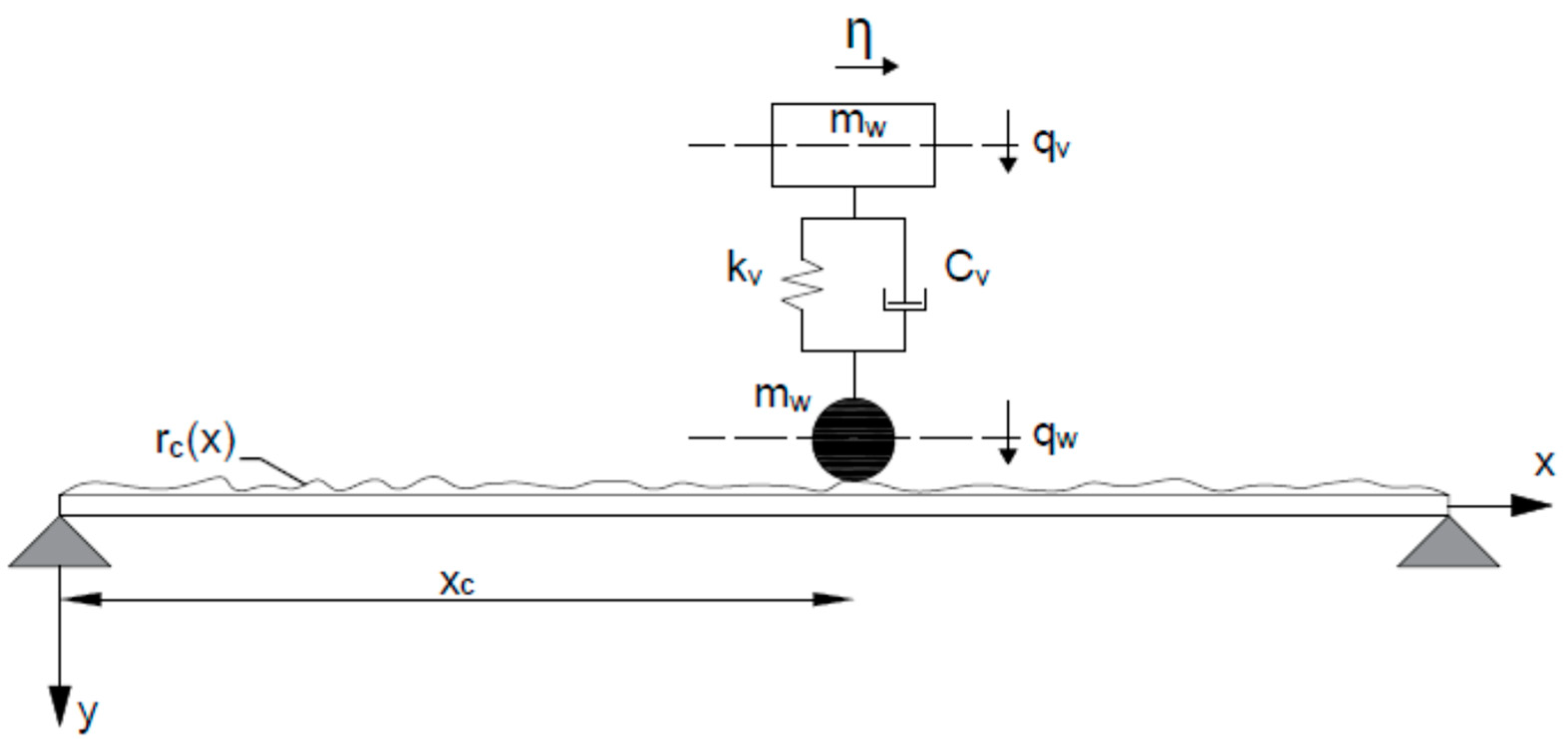
The model of a simply supported beam subjected to the passage of a single moving vehicle [34] (Figure 1) is here considered; the assumption about the structural configuration does not limit the generality of the discussion provided that the boundary conditions are adapted to different case studies.

From a dynamic standpoint, a sprung mass model can be adopted for a vehicle that moves along the bridge. This model consists of two lumped masses, one (m_v) representing the mass of the upper part of the vehicle, and one (m_w) associated to the wheels. The two masses are connected by a spring and a dashpot representing the vehicle suspensions. Considering a single vehicle moving on the beam with constant speed $\mathsf{\eta }$, the equation of motion is:

$${\mathrm{m}}_{\mathrm{v}}{\ddot{\mathrm{q}}}_{\mathrm{v}}+{\mathrm{c}}_{\mathrm{v}}\left({\dot{\mathrm{q}}}_{\mathrm{v}}-{\dot{\mathrm{q}}}_{\mathrm{w}}-{\dot{\mathrm{r}}}_{\mathrm{c}}\right)+{\mathrm{k}}_{\mathrm{v}}\left({\mathrm{q}}_{\mathrm{v}}-{\mathrm{q}}_{\mathrm{w}}-{\mathrm{r}}_{\mathrm{c}}\right)=0$$

(1)

where ${\mathrm{m}}_{\mathrm{v}}$, ${\mathrm{c}}_{\mathrm{v}}$, ${\mathrm{k}}_{\mathrm{v}}$ are respectively the sprung mass, the damping coefficient and the stiffness of the vehicle, and ${\ddot{\mathrm{q}}}_{\mathrm{v}}$, ${\dot{\mathrm{q}}}_{\mathrm{v}}$, ${\mathrm{q}}_{\mathrm{v}}$ are respectively the vertical acceleration, the velocity and the displacement of the vehicle; ${\dot{\mathrm{q}}}_{\mathrm{w}}$, ${\mathrm{q}}_{\mathrm{w}}$ are respectively the vertical velocity and displacement of the vehicle wheels, and ${\mathrm{r}}_{\mathrm{c}}$ and ${\dot{\mathrm{r}}}_{\mathrm{c}}$ represent the displacements due to the roughness of the road surface and its time derivative. Considering the equilibrium of forces at the contact point between the vehicle and the beam, which can be identified by the spatial coordinate ${\mathrm{x}}_{\mathrm{c}}\left(\mathrm{t}\right)$, the equation of motion can be expressed as:

$${\mathrm{m}}_{\mathrm{w}}{\ddot{\mathrm{q}}}_{\mathrm{w}}={\mathrm{f}}_{\mathrm{c}}+{\mathrm{c}}_{\mathrm{v}}\left({\dot{\mathrm{q}}}_{\mathrm{v}}-{\dot{\mathrm{q}}}_{\mathrm{w}}-{\dot{\mathrm{r}}}_{\mathrm{c}}\right)+{\mathrm{k}}_{\mathrm{v}}\left({\mathrm{q}}_{\mathrm{v}}-{\mathrm{q}}_{\mathrm{w}}-{\mathrm{r}}_{\mathrm{c}}\right)$$

(2)

where ${\mathrm{f}}_{\mathrm{c}}$ represents the contact force. Assuming perfect contact between the two systems and including the cubic Hermitian shape functions $\left\{\mathrm{N}\right\}$ and the bridge displacement vector ${\{\mathrm{u}}_{\mathrm{b}}\}$ in the problem, the following relations can be written:

$${\mathrm{q}}_{\mathrm{w}}={\left\{\mathrm{N}\right\}}^{\mathrm{T}}\left\{{\mathrm{u}}_{\mathrm{b}}\right\}$$

(3)

$${\dot{\mathrm{q}}}_{\mathrm{w}}={\left\{\mathrm{N}\right\}}^{\mathrm{T}}\left\{{\dot{\mathrm{u}}}_{\mathrm{b}}\right\}+\mathsf{\eta }{\left\{\mathrm{N}’\right\}}^{\mathrm{T}}\left\{{\mathrm{u}}_{\mathrm{b}}\right\}$$

(4)

$${\ddot{\mathrm{q}}}_{\mathrm{w}}={\left\{\mathrm{N}\right\}}^{\mathrm{T}}\left\{{\ddot{\mathrm{u}}}_{\mathrm{b}}\right\}+2\mathsf{\eta }{\left\{\mathrm{N}’\right\}}^{\mathrm{T}}\left\{{\dot{\mathrm{u}}}_{\mathrm{b}}\right\}+{\mathsf{\eta }}^2{\left\{\mathrm{N}’’\right\}}^{\mathrm{T}}\left\{{\mathrm{u}}_{\mathrm{b}}\right\}$$

(5)

where the superscripts $’$ and $’’$ respectively represent the first and second derivatives with respect to the spatial coordinate x, with:

$$\frac{\mathrm{d}\left\{\mathrm{N}\right\}}{\mathrm{dt}}=\frac{\mathrm{d}\left\{\mathrm{N}\right\}}{\mathrm{dx}}\frac{\mathrm{dx}}{\mathrm{dt}}=\mathsf{\eta }\frac{\mathrm{d}\left\{\mathrm{N}\right\}}{\mathrm{dx}}$$

(6)

The vector holding the cubic Hermitian shape functions can be expressed as:

$${\left\{\mathrm{N}\right\}}^{\mathrm{T}}=\left\{0\dots \left\{\mathrm{H}\left({\mathrm{x}}_{\mathrm{c}}\left(\mathrm{t}\right),\mathrm{t}\right)\right\}\dots 0\right\}$$

(7)

Replacing Equations (3)–(5) into Equation (1) and isolating the terms associated with the bridge displacement and velocity one obtains:

$${\mathrm{m}}_{\mathrm{v}}{\ddot{\mathrm{q}}}_{\mathrm{v}}+{\mathrm{c}}_{\mathrm{v}}\left({\dot{\mathrm{q}}}_{\mathrm{v}}-{\dot{\mathrm{r}}}_{\mathrm{c}}\right)+{\mathrm{k}}_{\mathrm{v}}\left({\mathrm{q}}_{\mathrm{v}}-{\mathrm{r}}_{\mathrm{c}}\right)-{\mathrm{c}}_{\mathrm{v}}{\left\{\mathrm{N}\right\}}^{\mathrm{T}}\left\{{\dot{\mathrm{u}}}_{\mathrm{b}}\right\}-({\mathrm{c}}_{\mathrm{v}}\mathsf{\eta }{\left\{\mathrm{N}’\right\}}^{\mathrm{T}}+{\mathrm{k}}_{\mathrm{v}}{\{\mathrm{N}\}}^{\mathrm{T}})\left\{{\mathrm{u}}_{\mathrm{b}}\right\}=0$$

(8)

In a similar way, inserting Equations (3)–(5) into Equation (2) the contact force value can be obtained as follows:

$${\mathrm{f}}_{\mathrm{c}}={\mathrm{m}}_{\mathrm{w}}{\left\{\mathrm{N}\right\}}^{\mathrm{T}}\left\{{\ddot{\mathrm{u}}}_{\mathrm{b}}\right\}+(2{\mathrm{m}}_{\mathrm{w}}\mathsf{\eta }{\left\{\mathrm{N}’\right\}}^{\mathrm{T}}+{\mathrm{c}}_{\mathrm{v}}{\left\{\mathrm{N}\right\}}^{\mathrm{T}})\left\{{\dot{\mathrm{u}}}_{\mathrm{b}}\right\}+({\mathrm{m}}_{\mathrm{w}}{\mathsf{\eta }}^2{\left\{\mathrm{N}’’\right\}}^{\mathrm{T}}+{\mathrm{c}}_{\mathrm{v}}\mathsf{\eta }{\{\mathrm{N}’\}}^{\mathrm{T}}+{\mathrm{k}}_{\mathrm{v}}{\{\mathrm{N}\}}^{\mathrm{T}})\left\{{\mathrm{u}}_{\mathrm{b}}\right\}-{\mathrm{c}}_{\mathrm{v}}\left({\dot{\mathrm{q}}}_{\mathrm{v}}-{\dot{\mathrm{r}}}_{\mathrm{c}}\right){\mathrm{k}}_{\mathrm{v}}\left({\mathrm{q}}_{\mathrm{v}}-{\mathrm{r}}_{\mathrm{c}}\right)$$

(9)

Taking into account that the equation of motion associated with the beam can be expressed as:

$$\left[{\mathrm{m}}_{\mathrm{b}}\right]\left\{{\ddot{\mathrm{u}}}_{\mathrm{b}}\right\}+ \left[{\mathrm{c}}_{\mathrm{b}}\right]\left\{{\dot{\mathrm{u}}}_{\mathrm{b}}\right\}+\left[{\mathrm{k}}_{\mathrm{b}}\right]\left\{{\mathrm{u}}_{\mathrm{b}}\right\}=-\left({\mathrm{f}}_{\mathrm{c}}+{\mathrm{m}}_{\mathrm{w}}\mathrm{g}+{\mathrm{m}}_{\mathrm{v}}\mathrm{g}\right)\left\{\mathrm{N}\right\}$$

(10)

where $\left[{\mathrm{m}}_{\mathrm{b}}\right]$, $\left[{\mathrm{c}}_{\mathrm{b}}\right]$ and $\left[{\mathrm{k}}_{\mathrm{b}}\right]$ are respectively the mass, damping and stiffness matrix of the beam, while the symbol $\mathrm{g}$ is used to indicate the acceleration of gravity, and inserting Equation (9) into Equation (10), the following equation is obtained:

$$\begin{gathered} (\left[{\mathrm{m}}_{\mathrm{b}}\right]+{\mathrm{m}}_{\mathrm{w}}{\left\{\mathrm{N}\right\}}^{\mathrm{T}}\left\{\mathrm{N}\right\})\left\{{\ddot{\mathrm{u}}}_{\mathrm{b}}\right\}+(\left[{\mathrm{c}}_{\mathrm{b}}\right]+2{\mathrm{m}}_{\mathrm{w}}\mathsf{\eta }{\left\{\mathrm{N}’\right\}}^{\mathrm{T}}\left\{\mathrm{N}\right\}+{\mathrm{c}}_{\mathrm{v}}{\left\{\mathrm{N}\right\}}^{\mathrm{T}}\left\{\mathrm{N}\right\})\left\{{\dot{\mathrm{r}}}_{\mathrm{b}}\right\}+(\left[{\mathrm{k}}_{\mathrm{b}}\right]+{\mathrm{m}}_{\mathrm{w}}{\mathsf{\eta }}^2{\left\{\mathrm{N}’’\right\}}^{\mathrm{T}}\left\{\mathrm{N}\right\} \\ +{\mathrm{c}}_{\mathrm{v}}\mathsf{\eta }{\left\{\mathrm{N}’\right\}}^{\mathrm{T}}\left\{\mathrm{N}\right\}+{\mathrm{k}}_{\mathrm{v}}{\{\mathrm{N}\}}^{\mathrm{T}}\left\{\mathrm{N}\right\})\left\{{\mathrm{u}}_{\mathrm{b}}\right\}={\mathrm{k}}_{\mathrm{v}}\left({\mathrm{q}}_{\mathrm{v}}-{\mathrm{r}}_{\mathrm{c}}\right)\left\{\mathrm{N}\right\}+{\mathrm{c}}_{\mathrm{v}}\left({\dot{\mathrm{q}}}_{\mathrm{v}}-{\dot{\mathrm{r}}}_{\mathrm{c}}\right)\left\{\mathrm{N}\right\}-\mathrm{g}\left({\mathrm{m}}_{\mathrm{w}}+{\mathrm{m}}_{\mathrm{v}}\right)\{\mathrm{N}\} \end{gathered}$$

(11)

Expressing the first-time derivative of the road surface roughness as follows:

$${\dot{\mathrm{r}}}_{\mathrm{c}}\left(\mathrm{x}\right)=\frac{{\mathrm{dr}}_{\mathrm{c}}\left(\mathrm{x}\right)}{\mathrm{dx}}\frac{\mathrm{dx}}{\mathrm{dt}}=\mathsf{\eta }\frac{{\mathrm{dr}}_{\mathrm{c}}\left(\mathrm{x}\right)}{\mathrm{dx}}$$

(12)

the equation of motion in matrix notation of the whole system can be written as:

$$\begin{gathered} \left[\begin{array}{ll}{\mathrm{m}}_{\mathrm{v}}\hfill & 0\hfill \\ 0\hfill & \left[{\mathrm{m}}_{\mathrm{b}}\right]+{\mathrm{m}}_{\mathrm{w}}{\left\{\mathrm{N}\right\}}^{\mathrm{T}}\left\{\mathrm{N}\right\}\hfill \end{array}\right]\left\{\begin{array}{l}{\ddot{\mathrm{q}}}_{\mathrm{v}}\hfill \\ \left\{{\ddot{\mathrm{u}}}_{\mathrm{b}}\right\}\hfill \end{array}\right\}+\left[\begin{array}{ll}{\mathrm{c}}_{\mathrm{v}}\hfill & -{\mathrm{c}}_{\mathrm{v}}{\left\{\mathrm{N}\right\}}^{\mathrm{T}}\hfill \\ -{\mathrm{c}}_{\mathrm{v}}\left\{\mathrm{N}\right\}\hfill & \left[{\mathrm{c}}_{\mathrm{b}}\right]+2{\mathrm{m}}_{\mathrm{w}}\mathsf{\eta }{\left\{\mathrm{N}’\right\}}^{\mathrm{T}}\left\{\mathrm{N}\right\}+{\mathrm{c}}_{\mathrm{v}}{\left\{\mathrm{N}\right\}}^{\mathrm{T}}\left\{\mathrm{N}\right\}\hfill \end{array}\right]\left\{\begin{array}{l}{\dot{\mathrm{q}}}_{\mathrm{v}}\hfill \\ \left\{{\dot{\mathrm{u}}}_{\mathrm{b}}\right\}\hfill \end{array}\right\} \\ +\left[\begin{array}{ll}{\mathrm{k}}_{\mathrm{v}}\hfill & -{\mathrm{k}}_{\mathrm{v}}{\left\{\mathrm{N}\right\}}^{\mathrm{T}}-{\mathrm{c}}_{\mathrm{v}}\mathsf{\eta }{\left\{\mathrm{N}’\right\}}^{\mathrm{T}}\hfill \\ -{\mathrm{k}}_{\mathrm{v}}\left\{\mathrm{N}\right\}\hfill & \left[{\mathrm{k}}_{\mathrm{b}}\right]+{\mathrm{m}}_{\mathrm{w}}{\mathsf{\eta }}^2{\left\{\mathrm{N}’’\right\}}^{\mathrm{T}}\left\{\mathrm{N}\right\}+{\mathrm{c}}_{\mathrm{v}}\mathsf{\eta }{\left\{\mathrm{N}’\right\}}^{\mathrm{T}}\left\{\mathrm{N}\right\}+{\mathrm{k}}_{\mathrm{v}}{\left\{\mathrm{N}\right\}}^{\mathrm{T}}\left\{\mathrm{N}\right\}\hfill \end{array}\right]\left\{\begin{array}{l}{\mathrm{q}}_{\mathrm{v}}\hfill \\ \left\{{\mathrm{u}}_{\mathrm{b}}\right\}\hfill \end{array}\right\} \\ =\left\{\begin{array}{l}{\mathsf{\eta }\mathrm{r}}_{\mathrm{c}}{\mathrm{c}}_{\mathrm{v}}+{\mathrm{r}}_{\mathrm{c}}{\mathrm{k}}_{\mathrm{v}}\hfill \\ -{\mathsf{\eta }\mathrm{r}}_{\mathrm{c}}{\mathrm{c}}_{\mathrm{v}}\left\{\mathrm{N}\right\}-{\mathrm{r}}_{\mathrm{c}}{\mathrm{k}}_{\mathrm{v}}\left\{\mathrm{N}\right\}-\mathrm{g}\left({\mathrm{m}}_{\mathrm{w}}+{\mathrm{m}}_{\mathrm{v}}\right)\left\{\mathrm{N}\right\}\hfill \end{array}\right\} \end{gathered}$$

(13)

The present model can be generalized to simulate the dynamic response of a bridge span in the case of random passages of multiple vehicles at constant speed [35]. Assuming that the mechanical characteristics of the i-th vehicle moving at constant speed ${\mathsf{\eta }}_{\mathrm{i}}$ are identified as ${\mathrm{m}}_{\mathrm{vi}}$, ${\mathrm{c}}_{\mathrm{vi}}$, ${\mathrm{k}}_{\mathrm{vi}}$ and ${\mathrm{m}}_{\mathrm{wi}}$, on the analogy with the previously adopted symbols, the position, velocity and acceleration of the $\mathrm{s}$ vehicles moving along the bridge can be gathered in the following vectors:

$$\left\{{\mathrm{q}}_{\mathrm{v}}\right\}={\{{\mathrm{q}}_{\mathrm{v}1},{\mathrm{q}}_{\mathrm{v}2},\cdots ,{\mathrm{q}}_{\mathrm{vs}}\}}^{\mathrm{T}}$$

(14)

$$\left\{{\dot{\mathrm{q}}}_{\mathrm{v}}\right\}={\{{\dot{\mathrm{q}}}_{\mathrm{v}1},{\dot{\mathrm{q}}}_{\mathrm{v}2},\cdots ,{\dot{\mathrm{q}}}_{\mathrm{vs}}\}}^{\mathrm{T}}$$

(15)

$$\left\{{\ddot{\mathrm{q}}}_{\mathrm{v}}\right\}={\{{\ddot{\mathrm{q}}}_{\mathrm{v}1},{\ddot{\mathrm{q}}}_{\mathrm{v}2},\cdots ,{\ddot{\mathrm{q}}}_{\mathrm{vs}}\}}^{\mathrm{T}}$$

(16)

Given the mechanical parameters and the mutual distance between two consecutive vehicles, it is possible to evaluate, for each time instant, the spatial coordinate ${\mathrm{x}}_{\mathrm{ci}}\left(\mathrm{t}\right)$ representing the distance travelled by the i-th vehicle on the bridge. The cubic Hermitian shape function for the i-th vehicle can be defined as follows:

$${\left\{{\mathrm{N}}_{\mathrm{i}}\right\}}^{\mathrm{T}}=\left\{0\dots \left\{\mathrm{H}\left({\mathrm{x}}_{\mathrm{ci}}\left(\mathrm{t}\right),\mathrm{t}\right)\right\}\dots 0\right\}$$

(17)

Under the assumption that each vehicle is coupled to the beam by its contact force, the equation of motion of the whole system can be expressed as:

$$\left[\begin{array}{ll}\left[{\mathrm{M}}_{\mathrm{vv}}\right]\hfill & \left[{\mathrm{M}}_{\mathrm{vb}}\right]\hfill \\ \left[{\mathrm{M}}_{\mathrm{bv}}\right]\hfill & \left[{\mathrm{M}}_{\mathrm{bb}}\right]\hfill \end{array}\right]\left\{\begin{array}{l}\left\{{\ddot{\mathrm{q}}}_{\mathrm{v}}\right\}\hfill \\ \left\{{\ddot{\mathrm{u}}}_{\mathrm{b}}\right\}\hfill \end{array}\right\}+\left[\begin{array}{ll}\left[{\mathrm{D}}_{\mathrm{vv}}\right]\hfill & \left[{\mathrm{D}}_{\mathrm{vb}}\right]\hfill \\ \left[{\mathrm{D}}_{\mathrm{bv}}\right]\hfill & \left[{\mathrm{D}}_{\mathrm{bb}}\right]\hfill \end{array}\right]\left\{\begin{array}{l}\left\{{\dot{\mathrm{q}}}_{\mathrm{v}}\right\}\hfill \\ \left\{{\dot{\mathrm{u}}}_{\mathrm{b}}\right\}\hfill \end{array}\right\}+\left[\begin{array}{ll}\left[{\mathrm{K}}_{\mathrm{vv}}\right]\hfill & \left[{\mathrm{K}}_{\mathrm{vb}}\right]\hfill \\ \left[{\mathrm{K}}_{\mathrm{bv}}\right]\hfill & \left[{\mathrm{K}}_{\mathrm{bb}}\right]\hfill \end{array}\right]\left\{\begin{array}{l}\left\{{\mathrm{q}}_{\mathrm{v}}\right\}\hfill \\ \left\{{\mathrm{u}}_{\mathrm{b}}\right\}\hfill \end{array}\right\}=\left\{\begin{array}{l}\left\{{\mathrm{f}}_{\mathrm{v}}\right\}\hfill \\ \left\{{\mathrm{f}}_{\mathrm{b}}\right\}\hfill \end{array}\right\}$$

(18)

or, in more compact matrix notation, as:

$$\left[{\mathrm{M}}_{\mathrm{sys}}\right]\left\{{\ddot{\mathrm{q}}}_{\mathrm{sys}}\right\}+\left[{\mathrm{D}}_{\mathrm{sys}}\right]\left\{{\dot{\mathrm{q}}}_{\mathrm{sys}}\right\}+\left[{\mathrm{K}}_{\mathrm{sys}}\right]\left\{{\mathrm{q}}_{\mathrm{sys}}\right\}=\left\{{\mathrm{F}}_{\mathrm{sys}}\right\}$$

(19)

where $\left[{\mathrm{M}}_{\mathrm{sys}}\right]$, $\left[{\mathrm{D}}_{\mathrm{sys}}\right]$, $\left[{\mathrm{K}}_{\mathrm{sys}}\right]$ are the $(\mathrm{s}+\mathrm{p}) \times (\mathrm{s} + \mathrm{p})$ mass, damping and stiffness matrices of the coupled vehicle-structure system, respectively, with s the total number of vehicles, while $\mathrm{p}$ denotes the number of degrees of freedom (DOFs) resulting from the finite element discretization of the beam representing the generic bridge span; $\left\{{\ddot{\mathrm{q}}}_{\mathrm{sys}}\right\}$, $\left\{{\dot{\mathrm{q}}}_{\mathrm{sys}}\right\}$ and $\left\{{\mathrm{q}}_{\mathrm{sys}}\right\}$ are the $(\mathrm{s} + \mathrm{p}) \times 1$ vectors representing the accelerations, velocities, and displacements of the whole system, respectively, and $\left\{{\mathrm{F}}_{\mathrm{sys}}\right\}$ is the $(\mathrm{s} + \mathrm{p}) \times 1$ force vector. The sub-matrices associated with the vehicles DOFs in Equation (18) are:

$$\left[{\mathrm{M}}_{\mathrm{vv}}\right]=\left[\begin{array}{lll}{\mathrm{m}}_{\mathrm{v}1}\hfill & \cdots \hfill & 0\hfill \\ ⋮\hfill & \ddots \hfill & ⋮\hfill \\ 0\hfill & \cdots \hfill & {\mathrm{m}}_{\mathrm{vs}}\hfill \end{array}\right]$$

(20)

$$\left[{\mathrm{D}}_{\mathrm{vv}}\right]=\left[\begin{array}{ccc}{\mathrm{c}}_{\mathrm{v}1}& \cdots & 0\\ ⋮& \ddots & ⋮\\ 0& \cdots & {\mathrm{c}}_{\mathrm{vs}}\end{array}\right]$$

(21)

$$\left[{\mathrm{K}}_{\mathrm{vv}}\right]=\left[\begin{array}{ccc}{\mathrm{k}}_{\mathrm{v}1}& \cdots & 0\\ ⋮& \ddots & ⋮\\ 0& \cdots & {\mathrm{k}}_{\mathrm{vs}}\end{array}\right]$$

(22)

while the sub-matrices associated with the bridge DOFs can be computed as:

$$\left[{\mathrm{M}}_{\mathrm{bb}}\right]=\left[{\mathrm{m}}_{\mathrm{b}}\right]+{\displaystyle \sum }_{\mathrm{i}=1}^{\mathrm{s}}{\mathrm{m}}_{\mathrm{wi}}\left\{{\mathrm{N}}_{\mathrm{i}}\right\}{\left\{{\mathrm{N}}_{\mathrm{i}}\right\}}^{\mathrm{T}}$$

(23)

$$\left[{\mathrm{D}}_{\mathrm{bb}}\right]=\left[{\mathrm{c}}_{\mathrm{b}}\right]+{\displaystyle \sum }_{\mathrm{i}=1}^{\mathrm{s}}2{\mathrm{m}}_{\mathrm{wi}}{\mathsf{\eta }}_{\mathrm{i}}\left\{{\mathrm{N}’}_{\mathrm{i}}\right\}{\left\{{\mathrm{N}}_{\mathrm{i}}\right\}}^{\mathrm{T}}+{\mathrm{c}}_{\mathrm{vi}}\left\{{\mathrm{N}}_{\mathrm{i}}\right\}{\left\{{\mathrm{N}}_{\mathrm{i}}\right\}}^{\mathrm{T}}$$

(24)

$$\left[{\mathrm{K}}_{\mathrm{bb}}\right]=\left[{\mathrm{k}}_{\mathrm{b}}\right]+{\displaystyle \sum }_{\mathrm{i}=1}^{\mathrm{s}}{\mathrm{m}}_{\mathrm{wi}}{\mathsf{\eta }}_{\mathrm{i}}^2\left\{{\mathrm{N}’’}_{\mathrm{i}}\right\}{\left\{{\mathrm{N}}_{\mathrm{i}}\right\}}^{\mathrm{T}}+{\mathrm{c}}_{\mathrm{vi}}{\mathsf{\eta }}_{\mathrm{i}}\left\{{\mathrm{N}’}_{\mathrm{i}}\right\}{\left\{{\mathrm{N}}_{\mathrm{i}}\right\}}^{\mathrm{T}}+{\mathrm{k}}_{\mathrm{vi}}\left\{{\mathrm{N}}_{\mathrm{i}}\right\}{\left\{{\mathrm{N}}_{\mathrm{i}}\right\}}^{\mathrm{T}}$$

(25)

The coupling between the beam and the $s$ vehicles is expressed by the following equations:

$$\left[{\mathrm{M}}_{\mathrm{vb}}\right]=\left[0\right]=\left[{\mathrm{M}}_{\mathrm{bv}}\right]$$

(26)

$${\mathrm{D}}_{\mathrm{vb}\left(\mathrm{i},*\right)}=-{\mathrm{c}}_{\mathrm{vi}}{\left\{{\mathrm{N}}_{\mathrm{i}}\right\}}^{\mathrm{T}}$$

(27)

$${\mathrm{D}}_{\mathrm{bv}\left(*,\mathrm{i}\right)}=-{\mathrm{c}}_{\mathrm{vi}}\left\{{\mathrm{N}}_{\mathrm{i}}\right\}$$

(28)

$${\mathrm{K}}_{\mathrm{vb}\left(\mathrm{i},*\right)}=-{\mathrm{k}}_{\mathrm{vi}}{\left\{{\mathrm{N}}_{\mathrm{i}}\right\}}^{\mathrm{T}}-{\mathrm{c}}_{\mathrm{vi}}{\mathsf{\eta }}_{\mathrm{i}}{\left\{{\mathrm{N}’}_{\mathrm{i}}\right\}}^{\mathrm{T}}$$

(29)

$$\left[{\mathrm{M}}_{\mathrm{vb}}\right]=\left[0\right]=\left[{\mathrm{M}}_{\mathrm{bv}}\right]$$

(30)

where the subscripts mark the correspondence with the submatrices of Equation (18), and the symbol $*$ denotes the entire row or column of the matrix. Finally, the load vector can be expressed as:

$${\mathrm{f}}_{\mathrm{vi}}={\mathrm{c}}_{\mathrm{vi}}{\mathrm{r}}_{\mathrm{ci}}{\mathsf{\eta }}_{\mathrm{i}}+{\mathrm{k}}_{\mathrm{vi}}{\mathrm{r}}_{\mathrm{ci}}$$

(31)

$$\left\{{\mathrm{f}}_{\mathrm{b}}\right\}=-{\displaystyle \sum }_{\mathrm{i}=1}^{\mathrm{s}}{\mathrm{c}}_{\mathrm{vi}}{\mathrm{r}}_{\mathrm{ci}}{\mathsf{\eta }}_{\mathrm{i}}\left\{{\mathrm{N}}_{\mathrm{i}}\right\}+{\mathrm{k}}_{\mathrm{vi}}{\mathrm{r}}_{\mathrm{ci}}\left\{{\mathrm{N}}_{\mathrm{i}}\right\}+\mathrm{g}\left({\mathrm{m}}_{\mathrm{wi}}+{\mathrm{m}}_{\mathrm{vi}}\right)\left\{{\mathrm{N}}_{\mathrm{i}}\right\}$$

(32)

Once the system of differential equations describing the dynamic behaviour of the systems has been defined, it can be solved by numerical methods.

In order to make the simulations as much realistic as possible, the road roughness profile should be also included in the model. The ISO 8608 Standard reports a procedure for the generation of the road roughness profiles. Eight classes of profiles are identified, ranging from the best (Class A) to the worst (Class H) road roughness. Based on the ISO 8608 Standard, the power spectral density (PSD) ${\mathrm{G}}_{\mathrm{d}}\left(\mathrm{n}\right)$ for the desired profile class can be computed as:

$${\mathrm{G}}_{\mathrm{d}}\left(\mathrm{n}\right)={\mathrm{G}}_{\mathrm{d}}\left({\mathrm{n}}_0\right){\left(\frac{\mathrm{n}}{{\mathrm{n}}_0}\right)}^{-2}$$

(33)

where $\mathrm{n}$ is the spatial frequency per meter, ${\mathrm{n}}_0 = 0.1\frac{\mathrm{cycle}}{\mathrm{m}}$, and the value of ${\mathrm{G}}_{\mathrm{d}}{(\mathrm{n}}_0)$ is reported in the ISO 8608 Standard as a function of the class of roughness. The road roughness profile can be generated afterwards through the following expression [36]:

$$\mathrm{r}\left(\mathrm{x}\right)={\displaystyle \sum }_{\mathrm{i}=1}^{\mathrm{Q}}{\mathrm{d}}_{\mathrm{i}}\cos \left({\mathrm{n}}_{\mathrm{i}}\mathrm{x}+{\mathsf{\Theta }}_{\mathrm{i}}\right)$$

(34)

where ${\mathrm{n}}_{\mathrm{i}}$ is the i-th spatial frequency, ${\mathsf{\Theta }}_{\mathrm{i}}$ is the random phase angle, and ${\mathrm{d}}_{\mathrm{i}}$ is the i-th amplitude computed as follows:

$${\mathrm{d}}_{\mathrm{i}}=\sqrt{2{\mathrm{G}}_{\mathrm{d}}\left(\mathrm{n}\right)\mathsf{\Delta }\mathrm{n}}$$

(35)

with $\mathsf{\Delta }\mathrm{n}$ denoting the sampling interval of the spatial frequency.

For the sake of clarity, a table listing the symbols used in the above section is provided in the Appendix A.

3. Modal Identification Results from Simulated Indirect Measurements

3.1. Simulation Parameters

The VBI model introduced in the previous section is herein applied to simulate the traffic induced vibration response of the bridge and its indirect measure through one or more instrumented vehicles parked on it. The simulated traffic induced vibrations are processed to assess the reliability and accuracy of modal parameter estimates obtained from indirect measurements collected by instrumented vehicle resting at given position. One-way motion of vehicles along the bridge is considered in the following; so, at the current stage, only road bridges consisting of two independent structures (one for each traffic direction) are analyzed. Nevertheless, as far as the Authors know, the extension of the VBI model to simulate traffic induced vibrations of the bridge due to random accesses of multiple vehicles with random characteristics and belonging to two different classes for modal identification based on indirect measurements is not reported in the literature and represents one of the main contributions of the present paper. In this perspective, it is worth noting that the generalized model shows relevant differences in terms of loading conditions and dynamics of the system with respect to the model simulating the bridge vibrations induced by trains consisting of a number of coaches placed at given distance and traveling at the same speed [15,37].

The modal properties of the bridge are estimated after having generated the time series of simulated indirect measurements. In order to simulate realistic inspection conditions, a few instrumented vehicles are considered. In the present proof-of-concept three vehicles are assumed to be resting on the bridge to demonstrate the effectiveness of the method and the possibility to get a rough estimation of the bridge mode shapes. The positions of the instrumented vehicles are assumed to be equally spaced at the quarters of the total length of the beam, while the moving vehicles acting as excitation source for the bridge are travelling at randomly selected constant velocities.

The discretization of the structure consisted of 60 Timoshenko beam finite elements [38], while the equations of motion were solved by using the Generalized-$\mathsf{\alpha }$ method, with ${\mathsf{\alpha }}_{\mathrm{m}}=\frac{1}{2}$ and ${\mathsf{\alpha }}_{\mathrm{f}}=\frac{1}{2}$ and a time step $\mathsf{\Delta }\mathrm{t}$ of 0.002 s. In agreement with well-established OMA good practices, the total duration of the acceleration records was longer than one thousand times the fundamental period of the structure [39]. Road roughness has been introduced into the VBI model to simulate as much realistically as possible the traffic induced vibration response of the bridge. Gaussian white noise has been added afterwards to the simulated dataset in order to assess the influence of measurement noise on the accuracy of estimates obtained from indirect measurements.

The FDD method has been applied for modal parameter estimation. It is a frequency domain, non-parametric method based on the Singular Value Decomposition (SVD) of the output PSD matrix. Structural resonances are identified from the singular value plots by peak picking; the corresponding singular vectors are good estimates of the corresponding mode shapes [40]. Hanning window and 50% overlap have been adopted in the computation of PSDs, resulting in a frequency resolution of 0.06 Hz.

The bridge considered in the simulations was schematized as a simply supported beam whose mechanical and geometric characteristics are shown in

Table 1. Geometry and material properties of the simply supported beam.

Length L (m)	Moment of Inertia I (m4)	Cross Section Area A (m2)	Young’s Modulus E (GPa)	Material Density ρ (kg/m3)	Mass Per Unit Length m (kg/m)	Shear Area As (m2)
30.00	2.71	7.30	35.22	2548.50	18604.05	2.40

. They yield the values of the fundamental natural frequencies reported in

Table 2. Fundamental natural frequencies of the beam.

Mode	Natural Frequency (Hz)
I	3.90
II	14.95
III	31.61

.

Rayleigh damping was assumed, and the model coefficients were obtained by considering a damping ratio of 1% for the first and the third mode.

The characteristics of the instrumented vehicles are shown in

Table 3. Properties of the instrumented vehicles.

Mass mv (kg)	Stiffness kv (kN/m)	Damping Coefficient cv (kN.s/m)	Wheel Mass mw (kg)
1500.00	20.00	3.00	50

.

Traffic on bridges is usually characterized by a variable number of vehicles with different dynamic characteristics. Hence, the characterization of traffic as a random phenomenon is performed by referring to the theory of probability. In the simulation of traffic induced vibrations of the bridge two groups of vehicles are considered: the first is representative of cars (small mass vehicles), while the second is representative of trucks (large mass vehicles). For each moving vehicle, its characteristics in terms of velocity, mass, damping, stiffness, wheel mass and mutual distance from the preceding vehicle have been randomly selected from uniform probability distributions. The upper and lower bounds of the characteristics of the two groups of vehicles defining the corresponding uniform probability distributions are reported in

Table 4. Lower and upper bounds of the properties of cars and trucks moving on the bridge.

Vehicle Group	Velocity (m/s)	Mass (kg)	Stiffness (kN/m)	Damping (kN.s/m)	Mutual Distance (m)
Cars	20.00–30.00	1000.00–3000.00	15.00–40.00	2.00–5.00	20.00–50.00
Trucks	15.00–25.00	5000.00–20,000.00	200.00–500.00	5.00–10.00	20.00–50.00

.

The masses of the wheels are kept fixed and equal to 50 kg for the cars and 100 kg for the trucks. In each simulation, a total number of 900 moving vehicles are considered, with a 1:1 ratio of vehicles belonging to the two different groups (450 cars and 450 trucks). Furthermore, since the vehicles in the starting conditions are not at rest, the arrival speed of the individual vehicle and the road roughness before entering the bridge have to be accounted for. To this aim, additional road segments were added before and after the bridge with length equal to the bridge span. Meanwhile, the mutual distance between two consecutive vehicles is the stretch of road that has to be travelled by the vehicle i-th in order for the vehicle i+1-th to start on the road segment that precedes the beam. Of course, given the different velocities involved, overtaking between vehicles is allowed.

The illustration of the simulation parameters allows to remark how an extensive definition of noise as disturbing signals is considered in this study, taking into the effect of increasing noise levels in the data (simulating the measurement noise and other random disturbances) as well as the need of discriminating the bridge modal characteristics from those of the instrumented vehicle. In addition, the relevant factors influencing the VBI (the road roughness, the different characteristics and velocities of vehicles randomly travelling on the simulated bridge, the initial velocity of travelling vehicles when approaching the bridge) are explicitly taken into account in the simulations.

3.2. Modal Identification Results

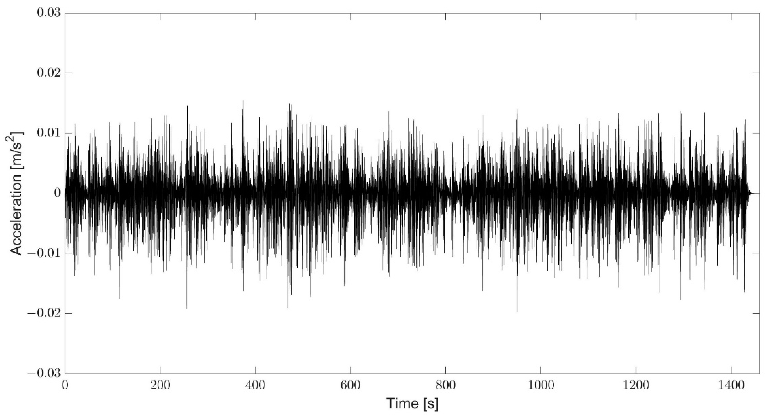
The traffic induced vibration response of the bridge has been simulated in the absence of road roughness and noise, first, in order to assess the effectiveness of the method in ideal conditions. The time histories of the accelerations measured by the instrumented vehicles (Figure 2) were 1460 s long: over the considered time window 900 vehicles were passing on the bridge.

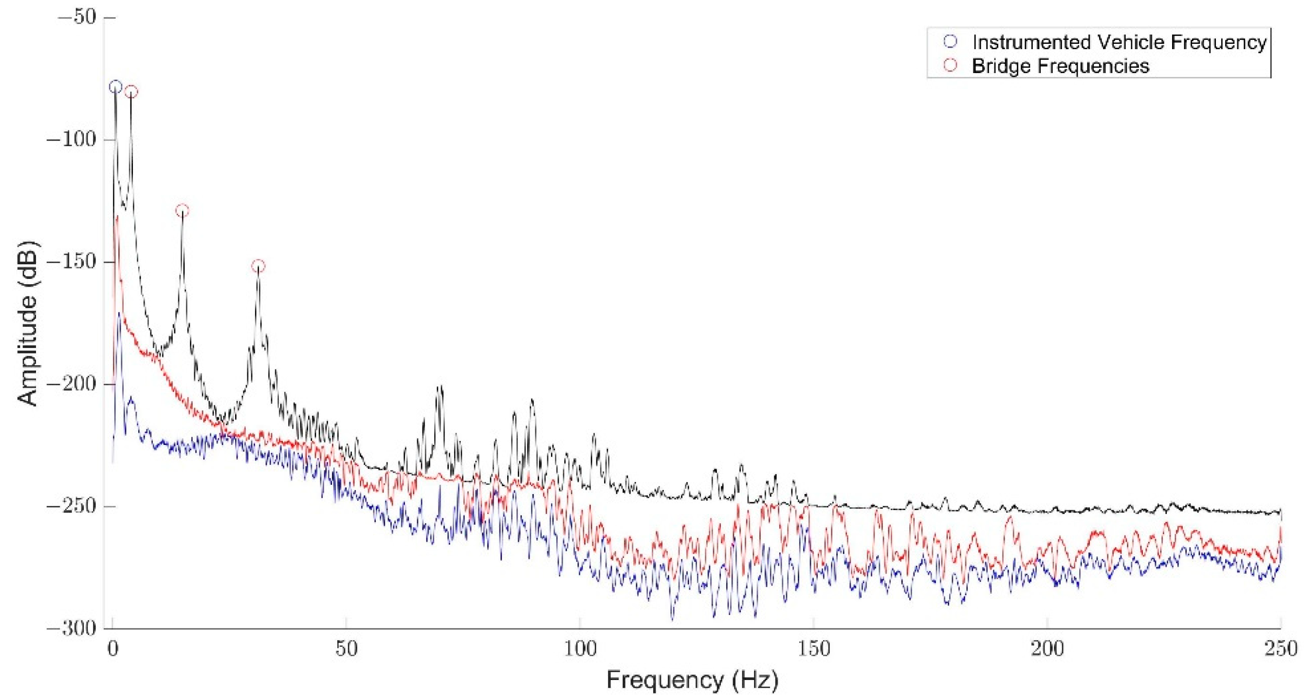
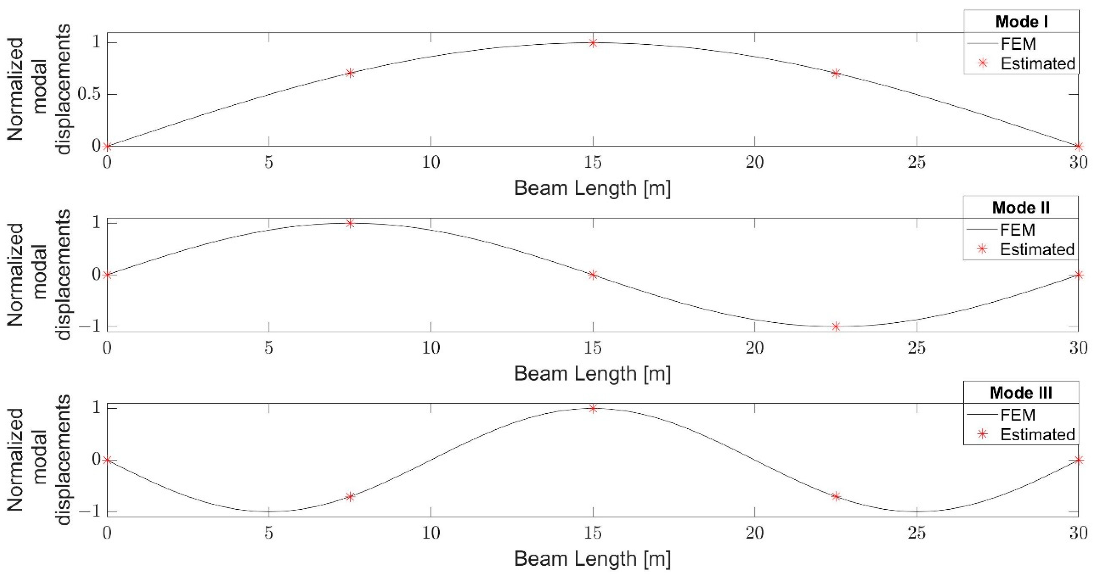
The singular value plots (Figure 3) obtained by applying FDD to the simulated data clearly show the superposition of the responses of the vehicle (characterized by the peak frequency of 0.6 Hz) and of the bridge. Nevertheless, if the dynamic properties of the vehicle at rest are known (for instance, because they have been preliminary obtained from a specific test), the natural frequencies of the bridge can be effectively identified and discriminated from the peaks associated to the response of the instrumented vehicle. Moreover, assuming that the measurements carried out by different vehicles are synchronized (for instance, by GPS signal), also the mode shapes of the bridge can be accurately estimated (Figure 4).

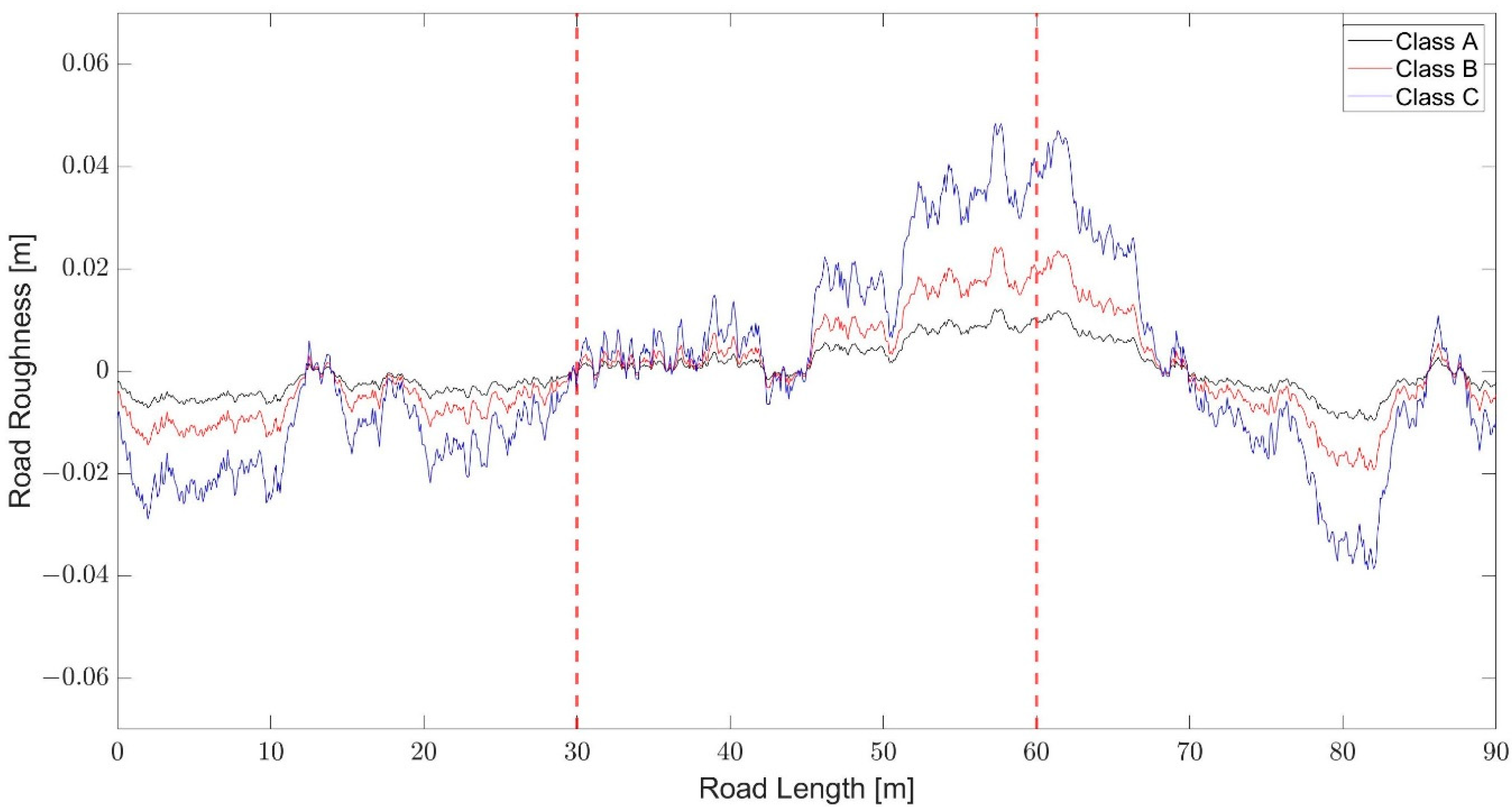
The road roughness has been introduced in the model, afterwards, in order to more realistically simulate the traffic induced vibration response of the bridge. Road roughness profiles of Class A, B, and C have been considered and modelled in agreement with the ISO 8608 Standard, which provides the values of ${\mathrm{G}}_{\mathrm{d}}\left({\mathrm{n}}_0\right)$ reported in

Table 5. Values of ${\mathrm{G}}_{\mathrm{d}}\left({\mathrm{n}}_0\right)$ for the considered road roughness profiles according to ISO 8608.

Profile Class	${\mathbf{G}}_{\mathbf{d}}\left({\mathbf{n}}_0\right)\mathit{·}{10}^{-6} \left(\raisebox{1ex}{${\mathbf{m}}^3$}\!\left/ \!\raisebox{-1ex}{$\mathbf{cycle}$}\right.\right)$
A	16
B	64
C	256

for the considered road profiles.

The simulated road roughness profiles for Class A, B, and C are shown in Figure 5, where the bridge corresponds to the middle part of the plots (from 30 m to 60 m), while the outer parts of the plots refer to the road segments introduced before and after the bridge to account for the effect of road roughness on the dynamic response of vehicles while entering the bridge.

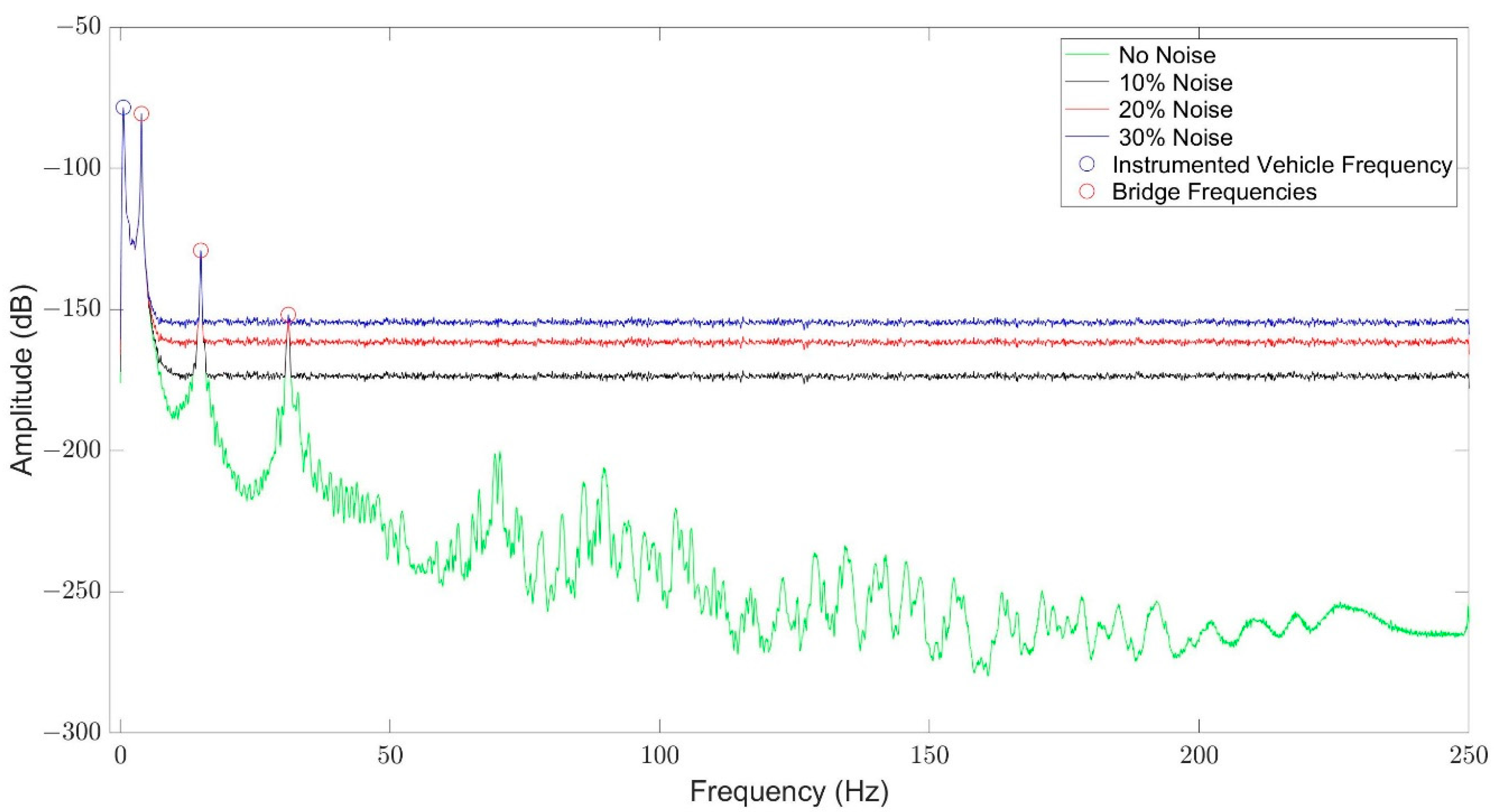
The traffic induced vibration response of the bridge has been simulated for the three different road profiles and increasing noise levels (10%, 20%, and 30%) in order to assess the performance of output-only modal identification from indirect measurements characterized by different signal-to-noise ratio. Gaussian white noise was therefore added to the simulated time series to account for the effect of measurement noise. While the results were consistent independently of the road profile, the presence of noise limited the identifiability of higher modes (

Table 6. Comparisons between the theoretical natural frequencies of the bridge and the identified values in the presence of road roughness (Class A) and increasing noise levels affecting the data.

Natural Frequency.	Theoretical	No Noise	10% Noise	20% Noise	30% Noise
f1 (Hz)	3.90	3.90	3.90	3.90	3.90
f2 (Hz)	14.95	14.88	14.88	14.88	14.88
f3 (Hz)	31.61	31.14	31.14	31.14	undetected

). In particular, the influence of increasing noise level in the data can be appreciated in Figure 6, showing the rise of the noise floor at increasing noise percentage. The obtained results remark the promising applicative perspectives of indirect measurements for the identification of the fundamental modal parameters by OMA techniques. However, the identifiability of higher, weakly excited modes appears limited even in the presence of relatively low noise level. In addition, the superposition of the dynamic responses of the instrumented vehicle and of the bridge requires the preliminary characterization of the dynamic properties of the vehicle and sensors characterized by high dynamic range in order to resolve with adequate accuracy the dominant response of the instrumented vehicle as well as the (typically low amplitude) response of the bridge.

In spite of the above-mentioned limitations, which can be easily overcome by preliminary dynamic testing of the instrumented vehicle (to characterize its dynamic response at ground) and adequate choice of sensors (above all in terms of dynamic range), the use of indirect measurements for OMA of bridges appears very attractive because tests become faster while minimizing the interference with the operating bridge as well as the risks related to sensor installation on a bridge open to traffic. Moreover, the obtained results confirm the effectiveness of the technique and the accuracy of estimates, at least with reference to the fundamental modes. Finally, if measurements carried out by multiple vehicles are GPS synchronized, accurate mode shape estimates (

Table 7. Comparisons between the theoretical normalized modal displacements of the bridge and the identified values in the presence of road roughness (Class A) and increasing noise levels affecting the data.

Instrumented Vehicle Position	Theoretical	No Noise	10% Noise	20% Noise	30% Noise
MODE I
7.50 m	0.71	0.71	0.71	0.71	0.71
15.00 m	1.00	1.00	1.00	1.00	1.00
22.50 m	0.71	0.71	0.71	0.71	0.71
MODE II
7.50 m	−1.00	−1.00	−0.99	−0.97	−0.96
15.00 m	0.00	0.00	0.01	0.02	0.03
22.50 m	1.00	1.00	1.00	1.00	1.00
MODE III
7.50 m	0.71	0.71	0.71	0.70	undetected
15.00 m	−1.00	−1.00	−1.00	−1.00	undetected
22.50 m	0.71	0.70	0.70	0.69	undetected

) can be obtained, too. Thus, OMA based on indirect vibration measurements by instrumented vehicles can be considered as a profitable alternative for dynamic testing of bridges in operational conditions.

4. Conclusions

The present paper reports the outcomes of a theoretical study aimed at assessing the performance of vehicles equipped with acceleration sensors as indirect measurement devices for OMA of bridges. The analysis has been carried out by applying a well-established OMA technique to the signals generated by a VBI model under random passages and characteristics of the multiple vehicles travelling on the bridge. The simulation of the traffic induced vibration response of the bridge under the random loading of multiple vehicles with different characteristics and including the effect of road roughness represents one of the contributions of the present study aimed at assessing the identifiability of the fundamental modes of bridges from indirect records of the structural response at increasing noise levels. The study started from recognizing that, for the usual bridge spans, the duration of vibration records collected by moving vehicles yields very poor frequency resolution in spectral analysis: as a consequence, attention has been focused on indirect measurements collected by vehicles at rest on the tested bridge; such sensor equipped vehicles might be the cars used by bridge inspectors for the periodic in-situ checks. The main findings of the study are here summarized:

• the data collected by the instrumented vehicles can be profitably processed to extract the fundamental modal properties of bridges in a fast and convenient way during periodic inspections with minimal interference on bridge operation;
• indirect measurements of the bridge response by instrumented vehicles at rest can be of adequate duration to ensure a fine frequency resolution in spectral analysis;
• accurate natural frequency and even mode shape estimates (if data from multiple vehicles are synchronized) can be obtained, at least with reference to the fundamental modes, while the identifiability of higher, weakly excited modes appears limited even in the presence of relatively low noise level;
• the superposition of the dynamic responses of the instrumented vehicle and of the bridge requires the preliminary characterization of the dynamic properties of the vehicle and sensors characterized by high dynamic range in order to resolve with adequate accuracy the dominant response of the instrumented vehicle as well as the (typically low amplitude) response of the bridge.

References

- Calvi, G.M.; Moratti, M.; O’Reilly, G.J.; Scattarreggia, N.; Monteiro, R.; Malomo, D.; Calvi, P.M.; Pinho, R. Once upon a Time in Italy: The Tale of the Morandi Bridge. Struct. Eng. Int. 2019, 29, 198–217. [Google Scholar] [CrossRef]
- Italian Ministry of Transportations and Infrastructures. Linee Guida per la Classificazione e Gestione del Rischio, la Valutazione Della Sicurezza ed il Monitoraggio dei Ponti Esistenti; Italian Ministry of Transportations and Infrastructures: Rome, Italy, 2020. [Google Scholar]
- Rainieri, C.; Fabbrocino, G. Operational Modal Analysis of Engineering Structures: Introduction and Guide for Applications; Springer: New York, NY, USA, 2014. [Google Scholar]
- Rainieri, C.; Fabbrocino, G. Automated output-only dynamic identification of civil engineering structures. Mech. Syst. Signal Process. 2010, 24, 678–695. [Google Scholar] [CrossRef]
- Rainieri, C.; Fabbrocino, G. Development and validation of an automated operational modal analysis algorithm for vibration-based monitoring and tensile load estimation. Mech. Syst. Signal Process. 2015, 60–61, 512–534. [Google Scholar] [CrossRef]
- Rainieri, C.; Magalhaes, F.; Gargaro, D.; Fabbrocino, G.; Cunha, A. Predicting the variability of natural frequencies and its causes by Second-Order Blind Identification. Struct. Health Monit. Int. J. 2019, 18, 486–507. [Google Scholar] [CrossRef]
- Malekjafarian, A.; McGetrick, P.J.; O’Brien, E.J. A review of indirect bridge monitoring using passing vehicles. Shock Vib. 2015, 2015, 286139. [Google Scholar] [CrossRef] [Green Version]
- Peeters, B.; Ventura, C.E. Comparative study of modal analysis techniques for bridge dynamic characteristics. Mech. Syst. Signal Process. 2003, 17, 965–988. [Google Scholar] [CrossRef]
- Meo, M.; Zumpano, G. On the optimal sensor placement techniques for a bridge structure. Eng. Struct. 2005, 27, 1488–1497. [Google Scholar] [CrossRef]
- Mahjoubi, S.; Barhemat, R.; Bao, Y. Optimal placement of triaxial accelerometers using hypotrochoid spiral optimization algorithm for automated monitoring of high-rise buildings. Autom. Constr. 2020, 118, 103273. [Google Scholar] [CrossRef]
- Liu, J.; Shen, H.; Narman, H.S.; Chung, W.A.; Lin, Z. A survey of mobile crowdsensing techniques: A critical component for the internet of things. ACM Trans. Cyber Phys. Syst. 2018, 2, 1–26. [Google Scholar] [CrossRef]
- Matarazzo, T.J.; Santi, P.; Pakzad, S.N.; Carter, K.; Ratti, C.; Moaveni, B.; Osgood, C.; Jacob, N. Crowdsensing framework for monitoring bridge vibrations using moving smartphones. Proc. IEEE 2018, 106, 577–593. [Google Scholar] [CrossRef]
- Fryba, L. Vibration of Solids and Structures under Moving Loads, 3rd ed.; Thomas Telford Ltd.: London, UK, 1999. [Google Scholar]
- Law, S.-S.; Zhu, X.-Q. Moving Loads-Dynamic Analysis and Identification Techniques; Structures and Infrastructures Book Series; RC Press: Boca Raton, CA, USA, 2011; Volume 8. [Google Scholar]
- Yang, Y.-B.; Yau, J.D.; Wu, Y.S. Vehicle-Bridge. In Interaction Dynamics with Applications to High-Speed Railways; World Scientific: Singapore, 2004. [Google Scholar]
- Yang, Y.-B.; Yau, J.-D. Vehicle-bridge interaction element for dynamic analysis. J. Struct. Eng. 1997, 123, 1512–1518. [Google Scholar] [CrossRef]
- Yang, Y.-B.; Lin, B.-H. Vehicle-bridge interaction analysis by dynamic condensation method. J. Struct. Eng. 1995, 121, 1636–1643. [Google Scholar] [CrossRef]
- Yang, Y.-B.; Lin, C.W.; Yau, J.D. Extracting bridge frequencies from the dynamic response of a passing vehicle. J. Sound Vib. 2004, 272, 471–493. [Google Scholar] [CrossRef]
- Lin, C.W.; Yang, Y.B. Use of a passing vehicle to scan the fundamental bridge frequencies: An experimental verification. Eng. Struct. 2005, 27, 1865–1878. [Google Scholar] [CrossRef]
- Yang, Y.B.; Chang, K.C. Extracting the bridge frequencies indirectly from a passing vehicle: Parametric study. Eng. Struct. 2009, 31, 2448–2459. [Google Scholar] [CrossRef]
- Yang, Y.B.; Chang, K.C. Extraction of bridge frequencies from the dynamic response of a passing vehicle enhanced by the EMD technique. J. Sound Vib. 2009, 322, 718–739. [Google Scholar] [CrossRef]
- Gonzalez, A.; Covian, E.; Madera, J. Determination of bridge natural frequencies using a moving vehicle instrumented with accelerometers and GPS. In Proceedings of the Ninth International Conference on Computational Structures Technology, Athens, Greece, 2–5 September 2008; Civil-Comp Press: Dun Eaglais, UK, 2008. [Google Scholar]
- McGetrick, P.J.; Gonzalez, A.; O’Brien, E.J. Theoretical investigation of the use of a moving vehicle to identify bridge dynamic parameters. Insight Non Destr. Test. Cond. Monit. 2009, 51, 433–438. [Google Scholar] [CrossRef] [Green Version]
- Malekjafarian, A.; O’Brien, E.J. Application of output-only modal method in monitoring of bridges using an instrumented vehicle. In Proceedings of the Civil Engineering Research in Ireland, Belfast, UK, 28–29 August 2014. [Google Scholar]
- Malekjafarian, A.; O’Brien, E.J. Identification of bridge mode shapes using short time frequency domain decomposition of the responses measured in a passing vehicle. Eng. Struct. 2014, 81, 386–397. [Google Scholar] [CrossRef] [Green Version]
- Siringoringo, D.M.; Fujino, Y. Estimating bridge fundamental frequency from vibration response of instrumented passing vehicle: Analytical and experimental study. Adv. Struct. Eng. 2012, 15, 417–433. [Google Scholar] [CrossRef]
- Ibrahim, S.R.; Brincker, R.; Asmussen, J.C. Modal parameter identification from responses of general unknown random inputs. In Proceedings of the 14th International Modal Analysis Conference (IMAC), Dearborn, MI, USA, 12–15 February 1996; pp. 446–452. [Google Scholar]
- Rainieri, C.; Fabbrocino, G.; Manfredi, G.; Dolce, M. Robust output-only modal identification and monitoring of buildings in the presence of dynamic interactions for rapid post-earthquake emergency management. Eng. Struct. 2012, 34, 436–446. [Google Scholar] [CrossRef]
- Oliva, J.; Goicolea, J.M.; Antolin, P.; Astiz, M.A. Relevance of a complete road surface description in vehicle–bridge interaction dynamics. Eng. Struct. 2013, 56, 466–476. [Google Scholar] [CrossRef]
- Gou, H.; Zhou, W.; Chen, G.; Bao, Y.; Pu, Q. In-situ test and dynamic response of a double-deck tied-arch bridge. Steel Compos. Struct. 2018, 27, 161–175. [Google Scholar]
- Yang, Y.-B.; Yang, J.P.; Zhang, B.; Wu, Y. Vehicle Scanning Method for Bridges; John Wiley & Sons Ltd.: Chichester, UK, 2020. [Google Scholar]
- Gonzalez, A. Vehicle-bridge dynamic interaction using finite element modelling. In Finite Element Analysis; Moratal, D., Ed.; InTech: Rijeka, Croatia, 2010. [Google Scholar]
- International Organization for Standardization. ISO 8608:2016 Mechanical Vibration—Road Surface Profiles—Reporting of Measured Data; International Organization for Standardization: Geneva, Switzerland, 2016. [Google Scholar]
- Yang, J.P.; Chen, B.H. Two-mass vehicle model for extracting bridge frequencies. Int. J. Struct. Stab. Dyn. 2018, 18, 1850056. [Google Scholar] [CrossRef]
- Yang, Y.B.; Wu, Y.S. A versatile element for analyzing vehicle–bridge interaction response. Eng. Struct. 2001, 23, 452–469. [Google Scholar] [CrossRef]
- Loprencipe, G.; Zoccali, P. Use of generated artificial road profiles in road roughness evaluation. J. Mod. Transp. 2017, 25, 24–33. [Google Scholar] [CrossRef] [Green Version]
- Yang, Y.B.; Yau, J.D. Resonance of high-speed trains moving over a series of simple or continuous beams with non-ballasted tracks. Eng. Struct. 2017, 143, 295–305. [Google Scholar] [CrossRef]
- Logan, D.L. Finite Element Method, 5th ed; Brooks/Cole: Pacific Grove, CA, USA, 2002. [Google Scholar]
- Brincker, R. Some elements of operational modal analysis. Shock Vib. 2014, 2014, 325839. [Google Scholar] [CrossRef]
- Brincker, R.; Zhang, L.; Andersen, P. Modal identification of output-only systems using frequency domain decomposition. Smart Mater. Struct. 2001, 10, 441–445. [Google Scholar] [CrossRef] [Green Version]
Figure 1.
Sprung mass model of a car moving on a bridge.
Figure 2.
Sample time history of the vertical acceleration measured by the instrumented vehicle.
Figure 3.
Singular value plots (no roughness, no noise). First singular values (black line), second singular values (red line), third singular values (blue line).
Figure 4.
Estimated vs. theoretical modal displacements (no roughness, no noise).
Figure 5.
Simulated road roughness profiles corresponding to Class A, B, and C.
Figure 6.
First singular value plots at increasing noise level.