
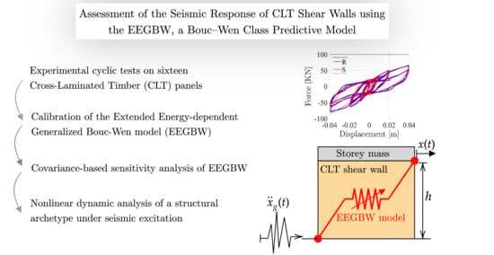
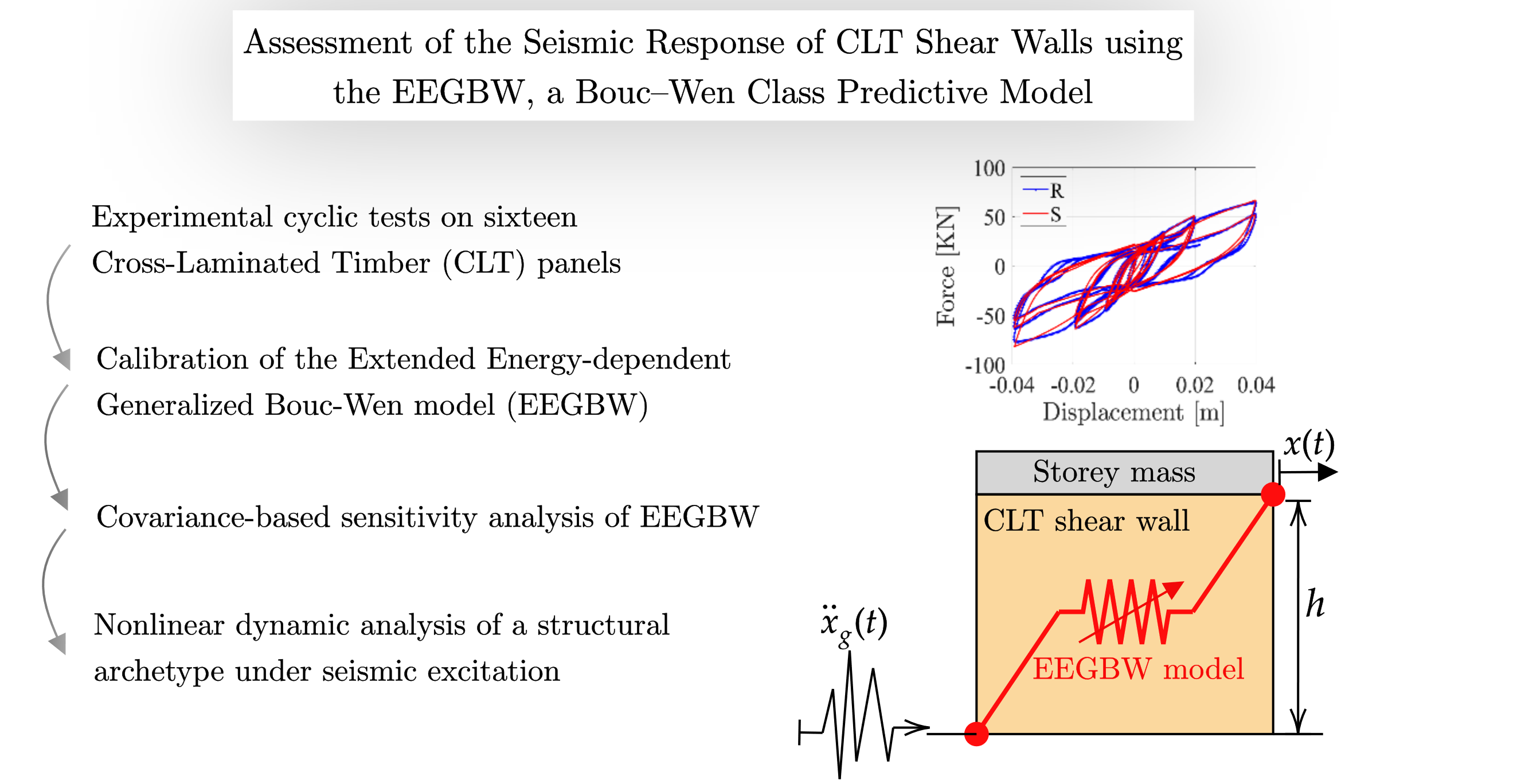
Assessment of the Seismic Response of CLT Shear Walls Using the EEGBW, a Bouc–Wen Class Predictive Model


Department of Civil, Architectural and Environmental Engineering, Università degli Studi dell’Aquila, Via Giovanni Gronchi n. 18, 67100 L’Aquila, Italy
*
Author to whom correspondence should be addressed.
Infrastructures 2021, 6(4), 55; https://0-doi-org.brum.beds.ac.uk/10.3390/infrastructures6040055
Submission received: 1 March 2021
/
Revised: 3 April 2021
/
Accepted: 4 April 2021
/
Published: 6 April 2021
(This article belongs to the Special Issue Advances in Structural Dynamics and Earthquake Engineering)
Abstract
:The paper presents an application of the Extended Energy-dependent Generalized Bouc–Wen model (EEGBW) to simulate the experimental cyclic response of Cross-Laminated Timber (CLT) panels. The main objectives of the paper are assessing the sensitivity of the quadratic error between experimental and numerical data to the EEGBW parameters, showing the fitting performance of the EEGBW model in matching the experimental cyclic response of CLT panels, highlighting the stability of the model in nonlinear dynamic analysis with seismic excitation. The research proves that the considered Bouc–Wen class hysteresis model can reproduce the hysteretic response of structural arrangements characterized by pinching and degradation phenomena. The model exhibits significant stability in nonlinear dynamic analysis with seismic excitation. The model’s stability and versatility endorse its application to simulate structural systems’ dynamic response when Finite Element modelling might be an impractical choice.
1. Introduction
Many of the recent research efforts in structural dynamics and earthquake engineering focus on predicting the inelastic response of real structures [1] or structural archetypes [2,3,4]. However, the analyses of rather elementary structures may require significant computational efforts. Consequently, the nonlinear dynamic analyses of more complicated systems are not feasible unless simplified methods are adopted. Among them, the use of empirical hysteresis models can significantly reduce the computational costs of nonlinear dynamic analysis. Empirical hysteresis models aim at reproducing the experimental response of the structural system without concern on the mechanics of materials: The model is empirical, i.e., it blindly matches the experimental data.
In timber structures, the structural dissipation is mainly localised in the connections. The empirical modelling of each connection using empirical hysteresis formulations rather than the Finite Element (FE) modelling of the connector can significantly ease the numerical simulations of complicated structural arrangements. In the scientific literature, there is a variety of empirical hysteresis models, and many models attempt to reproduce the complex phenomena of timber connections: pinching, strength degradation and stiffness degradation. The need to account for these phenomena entails more complex mathematical formulations.
There are two main categories of hysteresis models in structural engineering applications: differential and non-differential [5]. Differential models originate from Volterra’s pioneering studies at the beginning of the 20th century. Still, the history of hysteresis (i.e., rate-independent memory) is relatively short: Mathematical developments lag behind those of physicists and engineers. It was only in 1966 that hysteresis was first given a functional approach by Bouc, who introduced a differential hysteresis model later extended by Yi-Kwei Wen, Baber and Noori [6]. The Bouc–Wen–Baber–Noori BWBN model of hysteresis is one of the most used hysteretic models used to describe nonlinear hysteretic systems. This model can follow a wide range of hysteretic shapes. Foliente [7] modified the BWBN and applied the model to wood structures. Although the Bouc–Wen class models are the most used in structural engineering [8,9,10,11,12,13,14,15], the Bouc–Wen class models do not encompass all possible differential models. Mathematicians introduced the notion of hysteresis operator, which aims to unify all mathematical formulations possibly valid for an ample variety of hysteresis phenomena. The scientific literature is abundant of hysteresis models striving for generality and versatility [16]. However, most of the research in structural engineering, chiefly directed towards applications, does not deal with differential hysteresis models more evolved than the Bouc–Wen class ones and focalizes on non-differential formulations due to flaws and challenges in using these models. The Bouc–Wen class model, for instance, suffers from some shortcomings and require a consistent definition of the parameters to obtain upper-bounded results [17]. Additionally, the exact modelling of pinching, characterized by a notable boost in stiffness, may cause several convergence problems. Besides, the digital era’s ascension has lessened the energies of structural engineers devoted to the study of analytical models and praised more elementary approaches based on the use of piece-wise functions. Therefore, many scholars dedicated their research to algebraic or transcendental hysteresis models, which may have some stability advantages to the differential ones: They are generally faster and less computationally demanding. Algebraic hysteresis models refer to the formulations based on polynomial expressions, while transcendental ones originate from transcendental functions. Algebraic and transcendental models are non-differential models, compared to the well-known Bouc–Wen which is defined as a first ordinary differential equation.
In the field of timber engineering, a few scholars presented algebraic empirical hysteresis model, and most of them descend from the piece-wise definition of linear functions, like the models by Polensek and Laursen [18], the trilinear model by Rinaldin et al. [19] and the SAWS Material Model (OpenSees) [20]. Conversely, the CUREE model [21], the evolutionary parameter hysteretic model (EPHM) [22] and others [23,24] present nonlinear branches. Dolan [25] developed a transcendental hysteresis model based on four exponential functions that define the hysteretic curves. Moreover, [26] observed the significant stability of piece-wise definitions of the hysteresis models.
The current paper focuses on a Bouc–Wen class hysteresis model, proposed by [27], applied to the simulation of the lateral response of Cross-Laminated Timber (CLT) panels. The model originates from the hysteresis model by [28]. CLT is gaining popularity in residential and non-residential applications in Europe [29,30]. The novelty as well as the complexity of the seismic behaviour of CLT wall panels fed important experimental research activities [31,32,33,34]. Among the others, the most relevant were part of the SOFIE Project [35].
From the pioneering work of Foliente [7], the Bouc–Wen class hysteresis models have provided reliable tools in predicting the seismic behaviour of timber structural elements [8,9,10,11,12,13,36,37].
This paper converges on the Extended Energy-dependent Generalized Bouc–Wen model, initially presented by [27]. The research has three main objectives:
- Estimate the sensitivity of the quadratic error between simulated and experimental data to the EEGBW model’s parameters;
- Prove the model versatility in fitting the experimental cyclic response of CLT panels;
- Show the performance of the EEGBW model and the results of time integration given a seismic input.
The EEGBW model presents all drawbacks of differential hysteresis models in terms of stability. The reduced computational costs make it a valid alternative for the hysteresis modelling of connections and complex structural arrangements. The EEGBW model’s strength should derive from the interaction between the computational advantages of empirical hysteresis models and the versatility of FE analysis. The paper has the following organization. The second section presents the EEGBW model; the third section focuses on the modelling choices of a CLT panel as a single-degeree-of-freedom oscillator. The fourth and fifth sections present the experimental data and the result of the sensitivity analysis. The sixth and seventh sections present the results and conclusions.
2. Analytical Prediction Model
Theoretically, the response of a structural system may be formalized as follows:
| = Resisting force at a certain point of the wall panel; | |
| = The motion of all points of the all body (Panel); | |
| t | = Time. |
The constitutive law takes the form of a functional of the function; in short, not just the displacement of all points , but the entire history of displacements of all points () determines the resisting force at a certain time t. This is due to pinching and degradation phenomena.
The resisting force explicitly depends on as the mechanical properties are not uniform, being the structural system a peculiar assemble of timber and metal connectors. The resisting force depends on the motion of all points , not just on the ones nearby .
In particular, a Bouc–Wen hysteresis model is considered, given that empirical hysteresis laws are proved to be quite reliable tools in predicting the seismic behaviour of structural systems [8], under certain restrictions [14]. The EEGBW model provides an empirical representation of highly complex constitutive laws, in particular that of a CLT wall panel, where the coexistence of different resisting mechanisms makes a direct FEM approach a quite complex task. This paper focuses on the application of the EEGBW model to simulate the hysteretic response of CLT panels. Several scholars developed a more rigorous method in modelling the lateral response of Cross-Laminated Timber panels. In particular, the a few of them [38,39,40] followed an analytical approach based on the assumption of a suitable kinematic model. Still, the main drawback is the focus on the monotonic pseudo-static response by neglecting the hysteresis contribution. Given the complexity of a rigorous approach in describing the CLT system’s constitutive behaviour, an empirical hysteresis model may be preferable when dealing with nonlinear dynamic analyses. For an inelastic SDOF system with the Generalized Bouc–Wen model, the equation of motion can be expressed as
| m | = Mass; |
| x | = Displacement; |
| = Double derivative of x with respect to time; | |
| = Derivative of x with respect to time; | |
| = Resisting inelastic force; | |
| z | = Auxiliary variable that represents the inelastic behaviour. |
For a structural element described by a Bouc–Wen class model, the resisting force is written as
| = Post-to preyield stiffness ratio; | |
| = Initial stiffness. |
The evolution of z is determined by an auxiliary ordinary differential equation, which can be written in the form
| = Derivative of z with respect to time; | |
| A | = Parameter controlling the scale of the hysteresis loops; |
| n | = Parameter controlling the sharpness of the hysteresis loops; |
| = Nonlinear function controlling other shape features of the hysteresis loop. |
The functions for a Generalized Bouc–Wen model, reported in the scientific literature, are
- Generalized Bouc–Wen hysteresis model= Shape-control parameters.
- Generalized Bouc–Wen with pinching and without both strength and stiffness degradation
= Song’s shape-control parameters; = Pinching shape parameter, active when , and ; = Pinching shape parameter, active when , and ; = Sign functions time-history dependent; q = Fraction of the pinching level , ; = Time-dependent pinching level in terms of displacement. It is the maximum of the displacement function within the interval . - Generalized Bouc–Wen with pinching and both strength and stiffness degradation.Strength and stiffness degradation is accounted by setting the s parameters as linear functions of the dissipated hysteretic energy . The dissipated energy is given byIn particular the (6) becomeswhere the s parameters are set as linear function of the dissipated hysteretic energy as follows:
The EEGBW hysteresis model possesses all the important features observed in real structures, which include strength and stiffness degradation and pinching of the successive hysteresis loops.
3. Analytical Modelling of CLT Wall
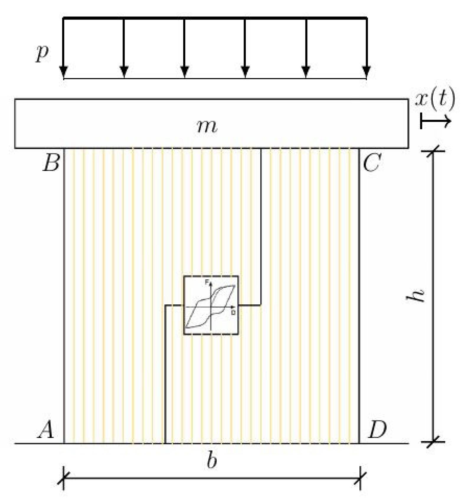
The authors adopted the archetype in Figure 1, as representative of the simplest structural unit in CLT buildings.
The CLT wall panel (A-B-C-D) is anchored to the foundation (A-D) with hold-downs and angle brackets. A static vertical load is applied on the wall, while a mass m stands on the top of the wall, as shown in Figure 1. The specimen in Figure 1 represents a standard structural configuration in CLT structure: a single panel anchored to the foundation by hold-downs and angle brackets. Reference [41] tested this sort of panels, depicted in Figure 2. Therefore, the model in Figure 1 is the idealization of the panel tested by [41], whose cyclic response is used to calibrate the EEGBW parameters in the current research. Considering the SDOF hysteretic system in Figure 1, the equation of motion coincides with the (2). All the information about the wall is expressed by the term, the wall configuration, the vertical connections, the static load, etc. The sole explicit terms in the (2) are the mass m and the coefficient of dynamic viscosity c. A global model of the wall is obtained, representative of the particular configuration under test.
4. Experimental Data
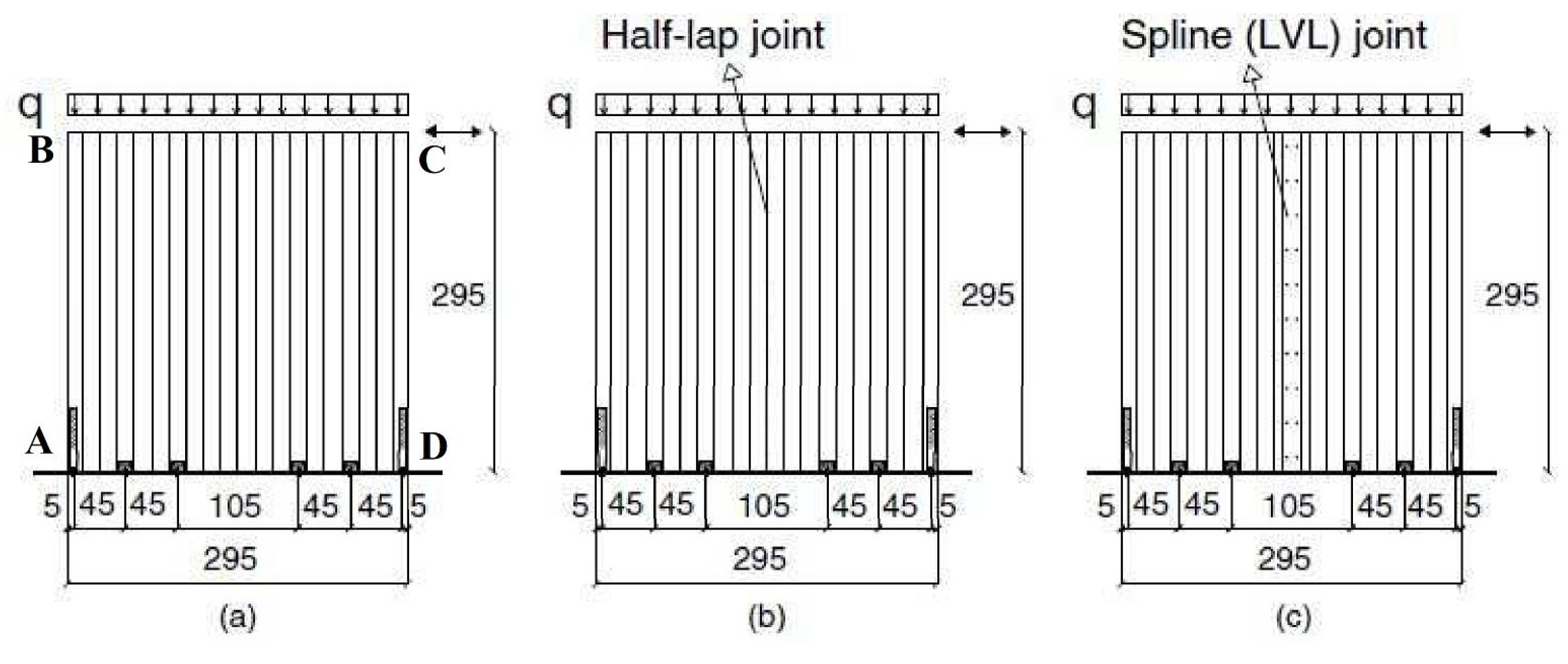
In the investigation, the authors used the experimental data published by [41]. Gavric et al. carried out experimental cyclic tests on 16 different CLT panels, featured by different structural layouts. Three wall configurations were investigated (Figure 2, Table 1):
- Wall configuration I (tests I.1-I.4): single wall panels with dimensions m (Figure 2a);
- Wall configuration II (tests II.1-II.4): two coupled wall panels with a half-lap joint (50 mm overlapping) and dimensions m for each panel (Figure 2b);
- Wall configuration III (tests III.1-III-8): two coupled wall panel with an laminated veneer lumber (LVL) spline joint ( mm LVL strip) and dimensions m for each panel (Figure 2c).
The estimation of the EEGBW model’s parameters descend from the opimization of the experimental data collected in point C, Figure 2. The following section reports the optimum parameters of the EEGBW model corresponding to the 16 different wall’s configurations.
5. Parameter Estimation and Sensitivity Analysis
The EEGBW model parameters are estimated by means of an OLS linear regression algorithm [42].
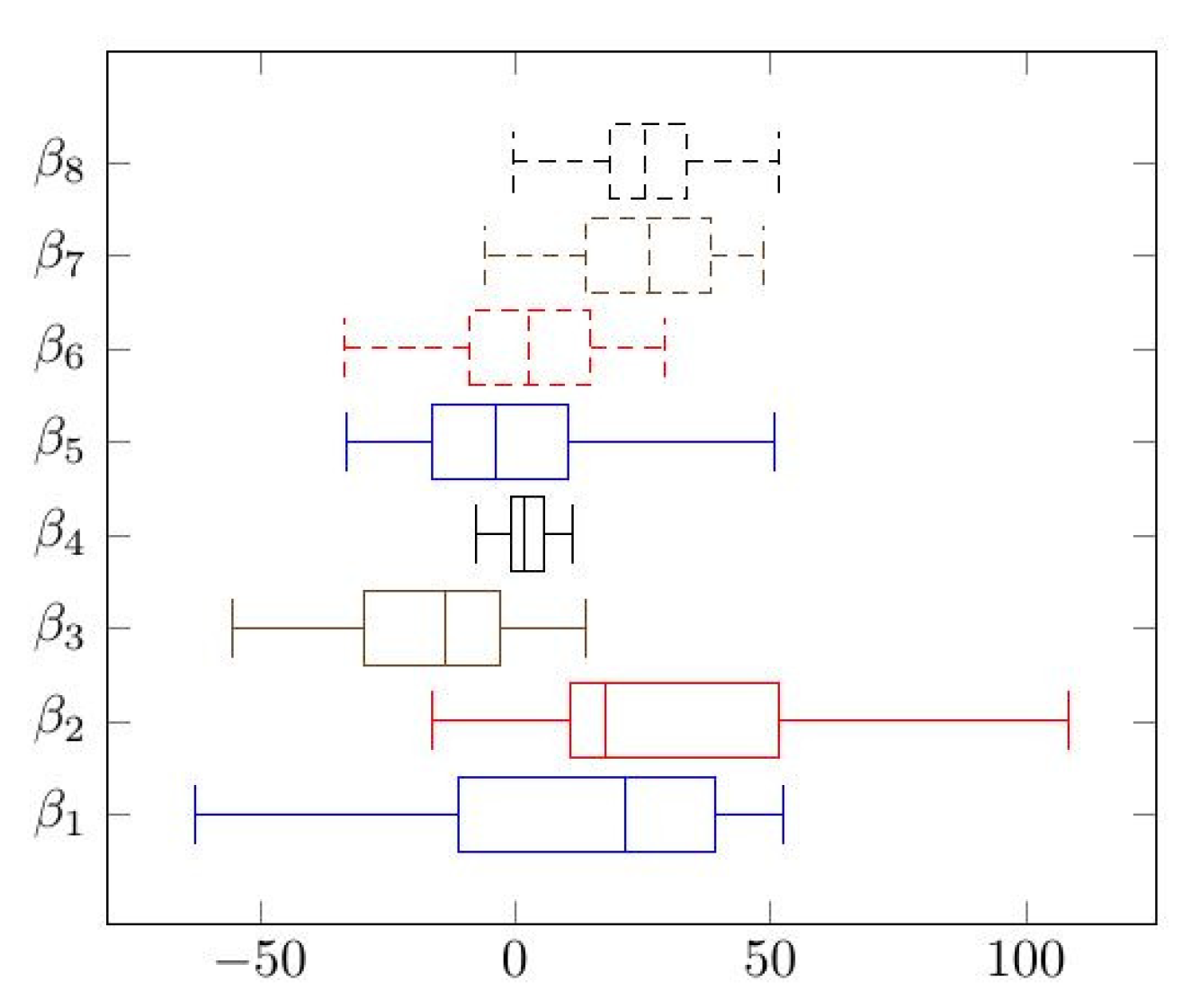
In particular, the n exponent, the parameters along with the coefficients are identified, for . The value of n, which minimizes the mean square error, is the same for all samples, equal to 0.9, while the and do show significant dispersion.
The EEGBW model faithfully describes the experimental data, as shown in Figure 5.
Despite the similarities exhibited by the different hysteresis loops, the identified parameters show a considerable dispersion.
A confirmation of the observed dispersion is drawn from a Variance-based Sensitivity Analysis [43]. A sensitivity index is in fact a number that gives quantitative information about the relative sensitivity of the model with respect to a selected set of parameters. A set of powerful global sensitivity indices is the group of Sobol indices [44].
Both the Sobol index and the total sensitivity index are computed in this paper. While measures the impact of varying a single parameter alone, measures the participation to the output variance of the selected parameter, including all variance caused by its interactions.
In short, the more different is the ranking generated by the two indexes, the more elaborate is the interaction between the parameters [45]. Information on parameter sensitivity is precious in system identification and system optimization. In the current paper, the sensitivity analysis function is the quadratic error function, that is, the quadratic error measured between the experimental data and the EEGBW parametric model of the first set of data.
The ranking generated by the Sobol indices does not match that by the total sensitivity indices ; Table 2. This might suggest that the interactions among the various parameters are very significant over the range specified (The specified ranges of the parameters are , and . Their choice is dictated by the variance exhibited by the parametric identification). As confirmed by Table 2, great variance of the EEGBW model parameters is expected. The EEGBW parameters, in fact, do not possess a full physical meaning. From their interactions, in fact, a wide range of possible hysteresis shapes is generated; Even the more insignificant variation of the experimental data does affect all the EEGBW parameters.
6. Results
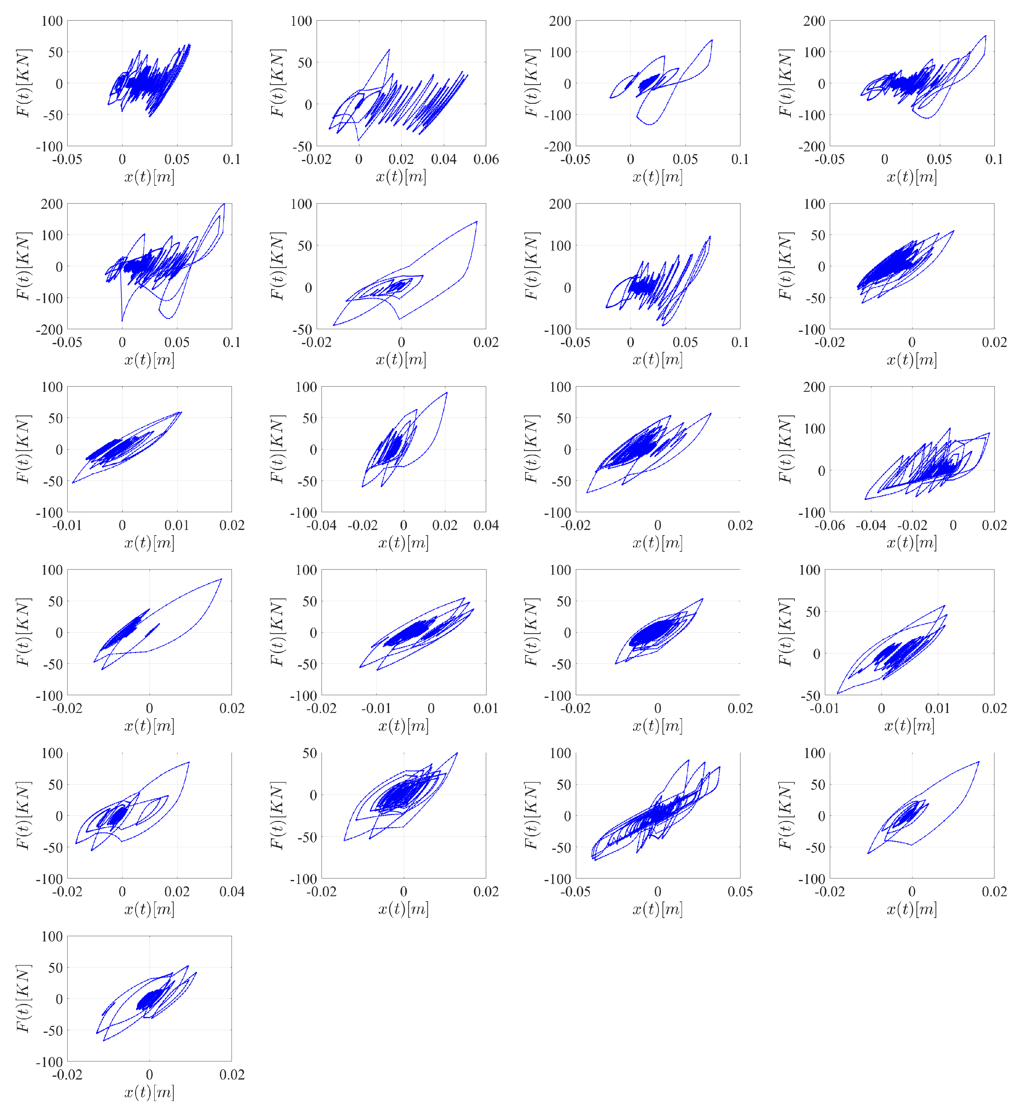
The 16 configurations of single and coupled cross-laminated wall panels, investigated by means of cyclic tests [41], are represented by the analytical EEGBW model and subjected to a series of 7 selected ground motion earthquakes Table 3. The mass m at the head of the panel is assumed equal to 8 KN, ie a fraction of the vertical load applied in quasi-static tests. The viscosity coefficient of timber structures is approximately 2%, as found by [1,46]. However, identifying the viscosity coefficient in operational conditions generally underestimates the actual viscosity coefficient at more significant displacements. Therefore, the authors adopted a 5% value, despite the results do not significantly depend on the viscosity coefficient due to the predominant contribution of hysteresis in energy dissipation. The second order non linear differential Equation (2) is integrated by means of the Runge-Kutta algorithm [47], Figure 6.
The CLT wall panels’ dissipative capacity is evaluated in terms of the maximum dissipated hysteretic energy. Thus the seismic performance of the different wall’s configurations (different anchoring systems, single and coupled walls, and different types and number of screws to connect the panels) is assessed.
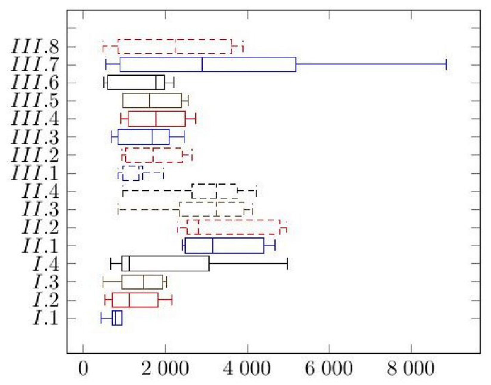
The layout and design of the joints is critical for the overall seismic behaviour of the structural system. In Figure 7, the box plot of the dissipated hysteresis energy is shown for the 16 different wall configurations.
- Effect of Vertical Connection between Adjacent Wall Panels. In the quasi-static tests, the different number of screws in the vertical joint between adjacent wall panels caused different kinematic behaviour of CLT walls, as well as different performance in terms of mechanical properties [41]. Despite Walls II.1 (20 screws in a half-lap joint) and III.1 (two lines of 20 screws in a LVL spline joint) have relatively stiff screwed connection, and their behaviour is not very close to that of single wall panels (configuration I), as in the experimental tests. More than the rigidity of the connection, due to the number of connectors, the different type of joint does cause global differences in the CLT panels’ seismic behaviour. From Figure 7, configuration I shows a lower dissipative capacity compared to the other two configurations. In particular configuration II and III, on average, boast a dissipative capacity greater than 176% and 48%, respectively, compared to the I configuration. The increase in ductility is guaranteed by the presence of the joint; in particular, the half-lap joint shows a more stable dissipative capacity, while the spline (LVL) joint is affected by a greater variance with respect to the particular earthquake. The reduction of the number of screws, resulting as the panels are rocking separately and not any more as one single panel, does not always affect the CLT wall behaviour. In particular, it does not sensibly modify the behaviour of CLT panels coupled with half-lap joint (II configuration), while it determines an increase in the dissipative capacity of about 26% in the third configuration. The LVL spline joint with fully threaded Wurth screws (Wall Tests III.7 and III.8) exhibits great variability of the response, revealing as a less reliable system in seismic conditions. While the global behaviour of the wall panels, in the quasi-static loading conditions, is mostly governed by metal connectors (hold-downs, angle brackets) rather than by the type of the selected vertical connection, the seismic behaviour is mostly governed by the type of vertical joint.
- Effect of the Number of Angle Brackets. Wall panel I.1 has only two angle brackets connecting the panel to the foundation. All the other walls have four angle brackets. The fundamental role played by the angle brackets in the CLT wall’s seismic response is clearly evident. With respect to the configuration with 2 angle brackets, an average increase of dissipated energy of about 60% is estimated. As evidenced by [41] in the quasi-static experimental tests, while the elastic stiffness of the wall I.1 is similar to the wall I.2 (single wall with four angle brackets), the maximum strength and ultimate displacement are both 47% lower with respect to Wall I.2. It can be inferred that the increase in resistance due to the angle brackets also determines an increase in the element’s dissipative capacity.
- Effect of Vertical Load. The vertical load does not significantly affect the dissipative capacity, with reference to the analysed configurations.
The outcomes of nonlinear dynamic analyses prove the model stability during numerical integration of Equation (2). The dissipated hysteretic energy values in Figure 7 are consistent with the values of ductility estimated from pseudo-static load tests. The parameters of the EEGBW model lack physical meaning. This fact represents an obstacle in extending the model to structural arrangements different from those used in model calibration. However, the model’s primary usefulness stands in the simulation of experimental cyclic response, which is difficult to reproduce with FE modelling. The EEGBW parameters are not related to the panel’s geometric features neither the mechanical parameters of timber: Empirical hysteresis models blindly match cyclic responses. Still, if empirical hysteresis models and FE are used together, the scholar can model the hysteretic response of more realistic structural arrangements with great accuracy and reduced computational costs. In timber structures, the dissipation capacity is localised by the connections. Therefore, the EEGBW model could be used to simulate the hysteretic response of the single connection via a nonlinear user-defined spring, while the panel via the Finite Element Method. In this case, the empirical hysteresis model can manifest its full potential, assisting direct FE modelling where hysteresis is localised in nonlinear springs, representing the structural connections. The authors developed the current research in Matlab. However, they are implementing the model in an Abaqus subroutine for more in-depth model validation.
7. Conclusions
The authors applied the EEGBW model to simulate the experimental cyclic response of Cross-Laminated Timber (CLT) panels tested. Accurately, they estimated the EEGBW parameters of sixteen structural configurations made by single and coupled cross-laminated wall panels. The estimation of the parameters originates from an Ordinary Least Squares (OLS) algorithm presented. Despite the similarities between the experimental data, the estimated parameters exhibited a significant dispersion. A variance-based sensitivity analysis based on Sobol indexes assessed each parameter’s effect on the quadratic error between experimental and numerical data. In a second step, the authors modelled the CLT panel as a single-degree-of-freedom system, whose resisting force is represented by the EEGBW model. They assessed the response of the sixteen-panel idealizations under a set of seven earthquakes using the Runge–Kutta algorithm. The hysteresis loops obtained from seismic excitation confirmed features reproduced in pseudo-static tests, pinching and degradation phenomena. In terms of the maximum dissipated hysteretic energy, the dissipative capacity is evaluated for the different CLT wall configurations. Interestingly, the vertical joint strongly affects the wall’s dissipative capacity; particularly, the half-lap joint determines a significant increase in the maximum dissipated energy. The Laminated Veneer Lumber (LVL) spline joint does not show a substantial difference compared to the configuration without the vertical joint. It could be believed that the presence of a vertical joint, favouring the sliding between the two panels, may increase ductility and energy dissipation. However, the sliding capacity and the type of strength and stiffness degradation of the particular vertical joint drive a CLT wall panel’s dissipative capacity. The EEGBW model is a so-called empirical model. Therefore, its significance and applicability are limited to the experimental data used for calibration. However, the model versatility could serve FE modelling of complex structural arrangements where the dissipative capacity is localised in the connection or structural nodes. These elements could be described by user-defined nonlinear spring in terms of the EEGBW model. The full model potential should emerge from the synergy between empirical hysteresis and FE modelling. Future research efforts will focus on implementing the EEGBW model as a new user-defined element in Abaqus to simulate the nonlinear dynamic response of more complicated structural arrangements.
Author Contributions
Conceptualization, methodology, software, validation, formal analysis, investigation, writing—original draft preparation, writing—review and editing, A.A.; supervision, M.F. All authors have read and agreed to the published version of the manuscript.
Funding
This research received no external funding.
Institutional Review Board Statement
Not applicable.
Informed Consent Statement
Not applicable.
Data Availability Statement
Data are available from the corresponding author upon reasonable request.
Conflicts of Interest
The authors declare no conflict of interest.
References
- Aloisio, A.; Pasca, D.; Tomasi, R.; Fragiacomo, M. Dynamic identification and model updating of an eight-storey CLT building. Eng. Struct. 2020, 213, 110593. [Google Scholar] [CrossRef]
- Aloisio, A.; Sejkot, P.; Iqbal, A.; Fragiacomo, M. An empirical transcendental hysteresis model for structural systems with pinching and degradation. Earthq. Eng. Struct. Dyn. 2021. [Google Scholar] [CrossRef]
- Aloisio, A.; Alaggio, R.; Fragiacomo, M. Equivalent Viscous Damping of Cross-Laminated Timber Structural Archetypes. J. Struct. Eng. 2021, 147, 04021012. [Google Scholar] [CrossRef]
- Aloisio, A.; Fragiacomo, M. Reliability-based overstrength factors of cross-laminated timber shear walls for seismic design. Eng. Struct. 2021, 228, 111547. [Google Scholar] [CrossRef]
- Visintin, A. Mathematical models of hysteresis. In Modelling and Optimization of Distributed Parameter Systems Applications to Engineering; Springer: Berlin/Heidelberg, Germany, 1996; pp. 71–80. [Google Scholar]
- Baber, T.T.; Wen, Y.K. Random vibration hysteretic, degrading systems. J. Eng. Mech. Div. 1981, 107, 1069–1087. [Google Scholar] [CrossRef]
- Foliente, G.C. Hysteresis modeling of wood joints and structural systems. J. Struct. Eng. 1995, 121, 1013–1022. [Google Scholar] [CrossRef] [Green Version]
- Sireteanu, T.; Giuclea, M.; Mitu, A. Identification of an extended Bouc–Wen model with application to seismic protection through hysteretic devices. Comput. Mech. 2010, 45, 431–441. [Google Scholar] [CrossRef]
- Ceravolo, R.; Demarie, G.V.; Erlicher, S. Instantaneous identification of Bouc-Wen-type hysteretic systems from seismic response data. In Key Engineering Materials; Trans Tech Publications Ltd.: Bäch, Switzerland, 2007; Volume 347, pp. 331–338. [Google Scholar]
- Jung, H.J.; Spencer, B.F., Jr.; Lee, I.W. Control of seismically excited cable-stayed bridge employing magnetorheological fluid dampers. J. Struct. Eng. 2003, 129, 873–883. [Google Scholar] [CrossRef]
- Bitaraf, M.; Hurlebaus, S.; Barroso, L.R. Active and semi-active adaptive control for undamaged and damaged building structures under seismic load. Comput.-Aided Civ. Infrastruct. Eng. 2012, 27, 48–64. [Google Scholar] [CrossRef]
- Karavasilis, T.L.; Kerawala, S.; Hale, E. Hysteretic model for steel energy dissipation devices and evaluation of a minimal-damage seismic design approach for steel buildings. J. Constr. Steel Res. 2012, 70, 358–367. [Google Scholar] [CrossRef]
- Sireteanu, T.; Giuclea, M.; Mitu, A.M. An analytical approach for approximation of experimental hysteretic loops by Bouc-Wen model. Proc. R. Acad. Ser. A 2009, 10, 4354. [Google Scholar]
- Ikhouane, F.; Mañosa, V.; Rodellar, J. Dynamic properties of the hysteretic Bouc-Wen model. Syst. Control Lett. 2007, 56, 197–205. [Google Scholar] [CrossRef]
- Aloisio, A.; De Angelo, M.; Alaggio, R.; D’Ovidio, G. Dynamic Identification of HTS Maglev Module for Suspended Vehicle by Using a Single-Degree-of-Freedom Generalized Bouc–Wen Hysteresis Model. J. Supercond. Nov. Magn. 2021, 34, 399–407. [Google Scholar] [CrossRef]
- Mayergoyz, I. The classical preisach model of hysteresis. In Mathematical Models of Hysteresis; Springer: Berlin/Heidelberg, Germany, 1991; pp. 1–63. [Google Scholar]
- Ismail, M.; Ikhouane, F.; Rodellar, J. The hysteresis Bouc-Wen model, a survey. Arch. Comput. Methods Eng. 2009, 16, 161–188. [Google Scholar] [CrossRef]
- Polensek, A.; Laursen, H.I. Seismic Behavior of Bending Components and Intercomponent Connections of Light Frame Wood Buildings; Oregon State University: Corvallis, OR, USA, 1984. [Google Scholar]
- Rinaldin, G.; Amadio, C.; Fragiacomo, M. A component approach for the hysteretic behaviour of connections in cross-laminated wooden structures. Earthq. Eng. Struct. Dyn. 2013, 42, 2023–2042. [Google Scholar] [CrossRef]
- Di Gangi, G.; Demartino, C.; Quaranta, G.; Monti, G. Dissipation in sheathing-to-framing connections of light-frame timber shear walls under seismic loads. Eng. Struct. 2020, 208, 110246. [Google Scholar] [CrossRef]
- Folz, B.; Filiatrault, A. Seismic analysis of woodframe structures. I: Model formulation. J. Struct. Eng. 2004, 130, 1353–1360. [Google Scholar] [CrossRef]
- Pang, W.; Rosowsky, D.; Pei, S.; Van de Lindt, J. Evolutionary parameter hysteretic model for wood shear walls. J. Struct. Eng. 2007, 133, 1118–1129. [Google Scholar] [CrossRef]
- Judd, J.P.; Fonseca, F.S. Analytical model for sheathing-to-framing connections in wood shear walls and diaphragms. J. Struct. Eng. 2005, 131, 345–352. [Google Scholar] [CrossRef] [Green Version]
- Blasetti, A.; Hoffman, R.; Dinehart, D. Simplified hysteretic finite-element model for wood and viscoelastic polymer connections for the dynamic analysis of shear walls. J. Struct. Eng. 2008, 134, 77–86. [Google Scholar] [CrossRef]
- Dolan, J.D. The Dynamic Response of Timber Shear Walls. Ph.D. Thesis, University of British Columbia, Vancouver, BC, Canada, 1989. [Google Scholar]
- Shen, Y.L.; Schneider, J.; Tesfamariam, S.; Stiemer, S.F.; Mu, Z.G. Hysteresis behavior of bracket connection in cross-laminated-timber shear walls. Constr. Build. Mater. 2013, 48, 980–991. [Google Scholar] [CrossRef]
- Aloisio, A.; Alaggio, R.; Köhler, J.; Fragiacomo, M. Extension of generalized bouc-wen hysteresis modeling of wood joints and structural systems. J. Eng. Mech. 2020, 146, 04020001. [Google Scholar] [CrossRef]
- Song, J.; Der Kiureghian, A. Generalized Bouc–Wen model for highly asymmetric hysteresis. J. Eng. Mech. 2006, 132, 610–618. [Google Scholar] [CrossRef] [Green Version]
- Popovski, M.; Karacabeyli, E. Seismic behaviour of cross-laminated timber structures. In Proceedings of the World Conference on Timber Engineering, Auckland, New Zealand, 15–19 July 2012. [Google Scholar]
- Sandoli, A.; D’Ambra, C.; Ceraldi, C.; Calderoni, B.; Prota, A. Sustainable Cross-Laminated Timber Structures in a Seismic Area: Overview and Future Trends. Appl. Sci. 2021, 11, 2078. [Google Scholar] [CrossRef]
- Shen, Y.; Schneider, J.; Tesfamariam, S.; Stiemer, S.F.; Chen, Z. Cyclic behavior of bracket connections for cross-laminated timber (CLT): Assessment and comparison of experimental and numerical models studies. J. Build. Eng. 2021, 39, 102197. [Google Scholar] [CrossRef]
- Barbosa, A.R.; Rodrigues, L.G.; Sinha, A.; Higgins, C.; Zimmerman, R.B.; Breneman, S.; Pei, S.; van de Lindt, J.W.; Berman, J.; McDonnell, E. Shake-table experimental testing and performance of topped and untopped cross-laminated timber diaphragms. J. Struct. Eng. 2021, 147, 04021011. [Google Scholar] [CrossRef]
- Mugabo, I.; Barbosa, A.R.; Sinha, A.; Higgins, C.; Riggio, M.; Pei, S.; van de Lindt, J.W.; Berman, J.W. System Identification of UCSD-NHERI Shake-Table Test of Two-Story Structure with Cross-Laminated Timber Rocking Walls. J. Struct. Eng. 2021, 147, 04021018. [Google Scholar] [CrossRef]
- Zhang, X.; Isoda, H.; Sumida, K.; Araki, Y.; Nakashima, S.; Nakagawa, T.; Akiyama, N. Seismic Performance of Three-Story Cross-Laminated Timber Structures in Japan. J. Struct. Eng. 2021, 147, 04020319. [Google Scholar] [CrossRef]
- Ceccotti, A.; Follesa, M.; Lauriola, M.; Sandhaas, C. SOFIE project–test results on the lateral resistance of cross-laminated wooden panels. In Proceedings of the First European Conference on Earthquake Engineering and Seismicity, Geneva, Switzerland, 3–8 September 2006; Volume 3. [Google Scholar]
- Goda, K.; Hong, H.; Lee, C. Probabilistic characteristics of seismic ductility demand of SDOF systems with Bouc-Wen hysteretic behavior. J. Earthq. Eng. 2009, 13, 600–622. [Google Scholar] [CrossRef]
- Pei, S.; Huang, D.; Berman, J.; Wichman, S. Simplified Dynamic Model for Post-tensioned Cross-laminated Timber Rocking Walls. Earthq. Eng. Struct. Dyn. 2021, 50, 845–862. [Google Scholar] [CrossRef]
- Casagrande, D.; Doudak, G.; Mauro, L.; Polastri, A. Analytical approach to establishing the elastic behavior of multipanel CLT shear walls subjected to lateral loads. J. Struct. Eng. 2018, 144, 04017193. [Google Scholar] [CrossRef]
- Nolet, V. Analytical Methodology to Predict the Behaviour of Multi-Panel CLT Shearwalls Subjected to Lateral Loads. Ph.D. Thesis, University of Ottawa, Ottawa, ON, Canada, 2017. [Google Scholar]
- Nolet, V.; Casagrande, D.; Doudak, G. Multipanel CLT shearwalls: An analytical methodology to predict the elastic-plastic behaviour. Eng. Struct. 2019, 179, 640–654. [Google Scholar] [CrossRef]
- Gavric, I.; Fragiacomo, M.; Ceccotti, A. Cyclic behavior of CLT wall systems: Experimental tests and analytical prediction models. J. Struct. Eng. 2015, 141, 04015034. [Google Scholar] [CrossRef]
- Aloisio, A.; Alaggio, R.; Fragiacomo, M. Dynamic identification of a masonry façade from seismic response data based on an elementary ordinary least squares approach. Eng. Struct. 2019, 197, 109415. [Google Scholar] [CrossRef]
- Aloisio, A.; Di Battista, L.; Alaggio, R.; Fragiacomo, M. Sensitivity analysis of subspace-based damage indicators under changes in ambient excitation covariance, severity and location of damage. Eng. Struct. 2020, 208, 110235. [Google Scholar] [CrossRef]
- Sobol, I.M. Sensitivity estimates for nonlinear mathematical models. Math. Model. Comput. Exp. 1993, 1, 407–414. [Google Scholar]
- Ma, F.; Zhang, H.; Bockstedte, A.; Foliente, G.C.; Paevere, P. Parameter analysis of the differential model of hysteresis. J. Appl. Mech. 2004, 71, 342–349. [Google Scholar] [CrossRef]
- Abrahamsen, R.; Bjertnaes, M.A.; Bouillot, J.; Brank, B.; Cabaton, L.; Crocetti, R.; Flamand, O.; Garains, F.; Gavric, I.; Germain, O.; et al. Dynamic Response of Tall Timber Buildings Under Service Load: The DynaTTB Research Program. In Proceedings of the XI International Conference on Structural Dynamics, EURODYN 2020, Athens, Greece, 22–24 June 2020. [Google Scholar]
- Dormand, J.R.; Prince, P.J. A family of embedded Runge-Kutta formulae. J. Comput. Appl. Math. 1980, 6, 19–26. [Google Scholar] [CrossRef] [Green Version]
Figure 1.
SDOF Idealization of a CLT wall panel through a SDOF Mechanical Model.

Figure 2.
Configuration of the three panels typologies tested by [41], where (a), (b) and (c) identify the I, II and III wall configurations, respectively.
Figure 2.
Configuration of the three panels typologies tested by [41], where (a), (b) and (c) identify the I, II and III wall configurations, respectively.

Figure 3.
Box plot of the system’s parameters from the OLS Identification.

Figure 4.
Box plot of the system parameters from the OLS Identification.
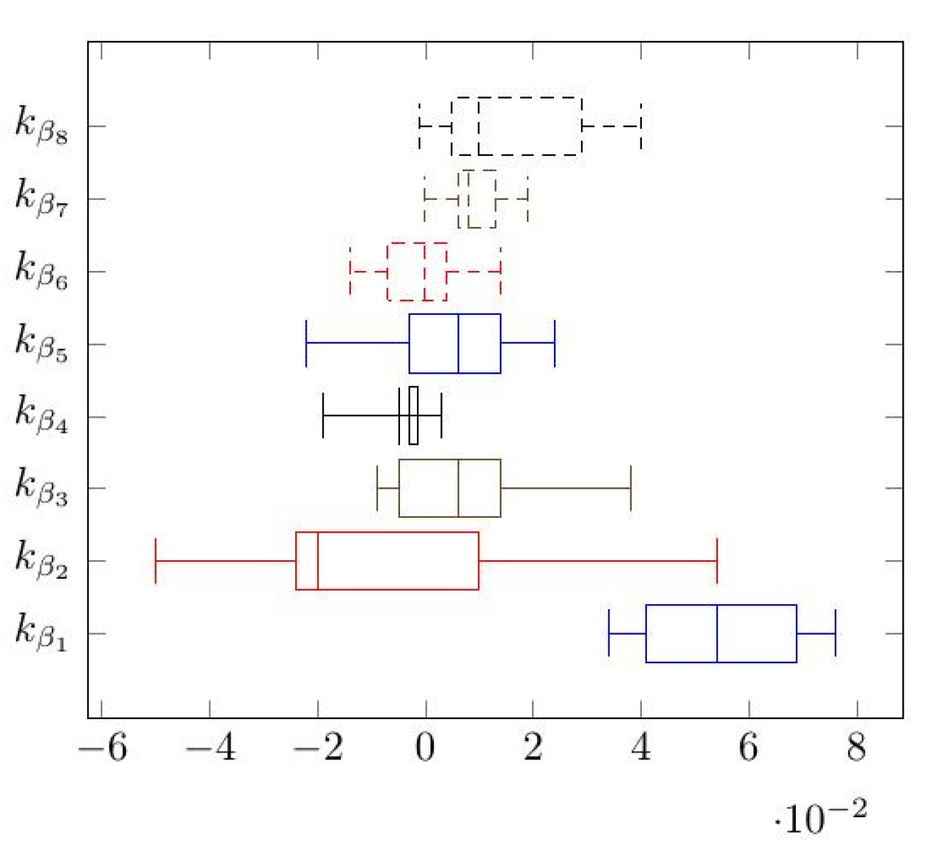
Figure 5.
Superposition of the experimental (continuous) and simulated (dashed) hysteresis loops.
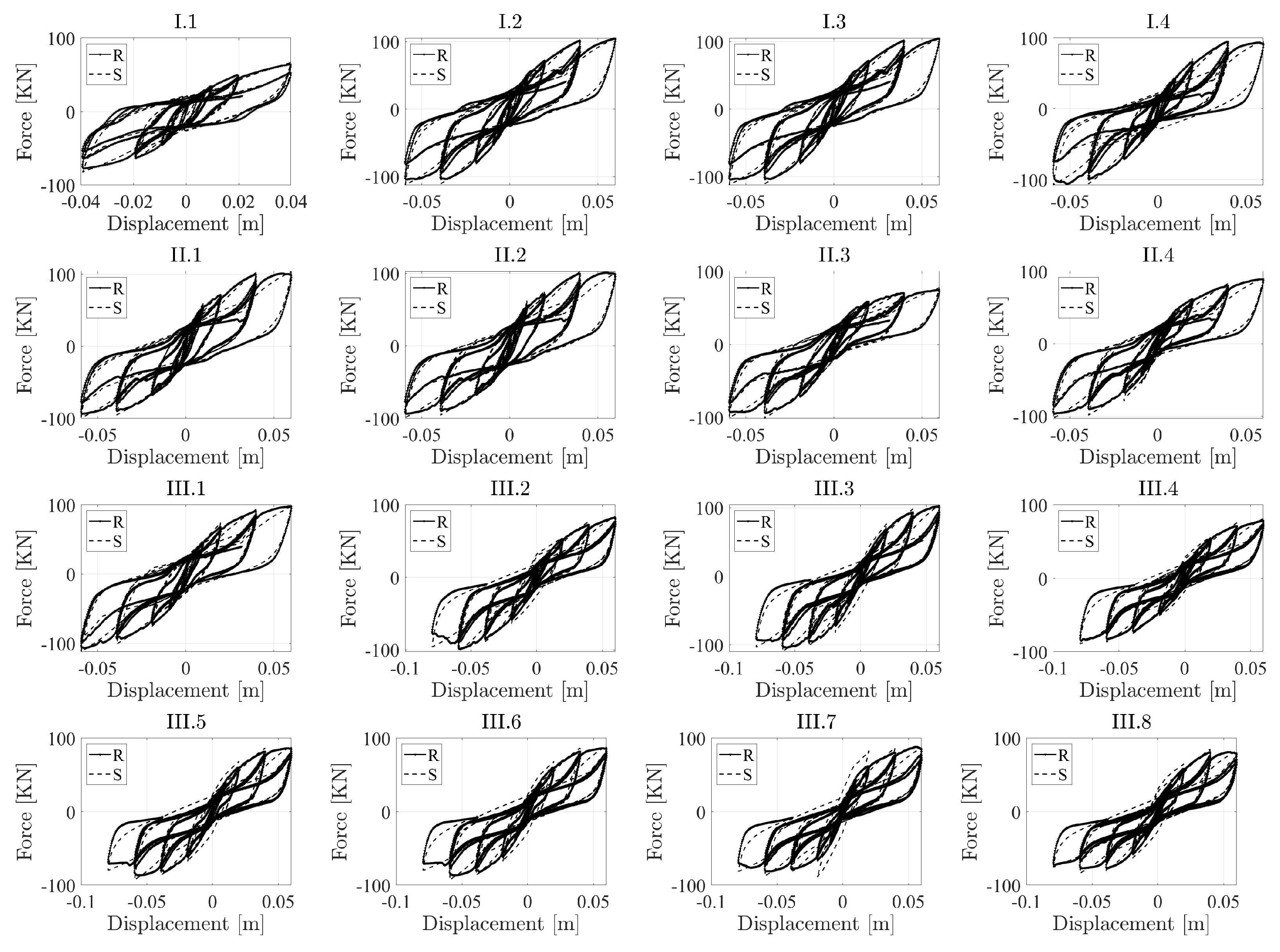
Figure 6.
Hysteresis loops of the first CLT wall configuration. From (a–g), (h–n) and (o–u), the responses of the I.1, I.2 and I.3 CLT wall configurations, respectively, are reported. Each set corresponds to the particular system’s response to the 7 selected accelerograms.
Figure 6.
Hysteresis loops of the first CLT wall configuration. From (a–g), (h–n) and (o–u), the responses of the I.1, I.2 and I.3 CLT wall configurations, respectively, are reported. Each set corresponds to the particular system’s response to the 7 selected accelerograms.

Figure 7.
Dissipated hysteretic energy in KJ for the 16 different wall configurations, subjected to a series of selected accelerograms.
Figure 7.
Dissipated hysteretic energy in KJ for the 16 different wall configurations, subjected to a series of selected accelerograms.


Table 1.
Wall configurations tested [41].
Table 1.
Wall configurations tested [41].
| Test Number | Number of Hold–Downs | Number of Angle Brackets | Number of Screws in Vertical Joints | Vertical Load (kN/m) |
|---|---|---|---|---|
| I.1 | 2 | 2 | - | 18.5 |
| I.2 | 2 | 4 | - | 18.5 |
| I.3 | 2 | 4 | - | 9.25 |
| I.4 | 2 | 4 | - | 18.5 |
| II.1 | 2 | 4 | 20 | 18.5 |
| II.2 | 2 | 4 | 20 | 18.5 |
| II.3 | 2 | 4 | 10 | 18.5 |
| II.4 | 4 | 4 | 5 | 18.5 |
| III.1 | 2 | 4 | 2 × 20 | 18.5 |
| III.2 | 2 | 4 | 2 × 10 | 18.5 |
| III.3 | 4 | 4 | 2 × 5 | 18.5 |
| III.4 | 2 | 4 | 2 × 10 | 18.5 |
| III.5 | 2 | 4 | 2 × 10 | 18.5 |
| III.6 | 2 | 4 | 2 × 10 | 0 |
| III.7 | 2 | 4 | 2 × 10 | 18.5 |
| III.8 | 2 | 4 | 2 × 10 | 18.5 |
Table 2.
Parameter sensitivity ranking of the EEGBW model.
| Global Analysis | ||||
|---|---|---|---|---|
| Parameter | Sobol Index | Total Effect Index | ||
| w | Rank | Rank | ||
| 0.00083 | 12 | 0.75494 | 8 | |
| 0.00098 | 6 | 0.66063 | 12 | |
| 0.00055 | 15 | 0.84244 | 4 | |
| 0.00019 | 16 | 0.86705 | 2 | |
| 0.00145 | 4 | 0.67748 | 10 | |
| 0.00246 | 2 | 0.77378 | 6 | |
| 0.00093 | 8 | 0.65725 | 15 | |
| 0.00092 | 4 | 0.65402 | 17 | |
| 0.00083 | 13 | 0.75492 | 9 | |
| 0.00091 | 11 | 0.66061 | 13 | |
| 0.00057 | 14 | 0.84244 | 5 | |
| 0.00011 | 17 | 0.86706 | 3 | |
| 0.00141 | 5 | 0.67744 | 11 | |
| 0.00242 | 3 | 0.77376 | 7 | |
| 0.00092 | 9 | 0.65726 | 14 | |
| 0.00094 | 10 | 0.65401 | 16 | |
| n | 0.06762 | 1 | 0.99443 | 1 |
| 0.0843 | 6.2277 | |||
Table 3.
List of the earthquakes adopted in the analysis.
| Name | Areas Affected | Year | Mw | PGA [m/s] | |
|---|---|---|---|---|---|
| 1 | El Centro | United States, Mexico | 1940 | 6.9 | 3.50 |
| 2 | Erzican | Erzincan Province, Turkey | 1939 | 7.8 | 5.03 |
| 3 | Kobe | Japan | 1995 | 6.9 | 6.76 |
| 4 | L’Aquila | Italy | 2009 | 6.3 | 6.63 |
| 5 | Northridge | Southern California, United States | 1994 | 6.7 | 5.51 |
| 6 | Loma Prieta | San Francisco, United States | 1989 | 6.9 | 6.55 |
| 7 | Parkfield | California, United States | 2004 | 6.0 | 4.96 |
Publisher’s Note: MDPI stays neutral with regard to jurisdictional claims in published maps and institutional affiliations. |
© 2021 by the authors. Licensee MDPI, Basel, Switzerland. This article is an open access article distributed under the terms and conditions of the Creative Commons Attribution (CC BY) license (https://creativecommons.org/licenses/by/4.0/).
Share and Cite
MDPI and ACS Style
Aloisio, A.; Fragiacomo, M. Assessment of the Seismic Response of CLT Shear Walls Using the EEGBW, a Bouc–Wen Class Predictive Model. Infrastructures 2021, 6, 55. https://0-doi-org.brum.beds.ac.uk/10.3390/infrastructures6040055
AMA Style
Aloisio A, Fragiacomo M. Assessment of the Seismic Response of CLT Shear Walls Using the EEGBW, a Bouc–Wen Class Predictive Model. Infrastructures. 2021; 6(4):55. https://0-doi-org.brum.beds.ac.uk/10.3390/infrastructures6040055
Chicago/Turabian StyleAloisio, Angelo, and Massimo Fragiacomo. 2021. "Assessment of the Seismic Response of CLT Shear Walls Using the EEGBW, a Bouc–Wen Class Predictive Model" Infrastructures 6, no. 4: 55. https://0-doi-org.brum.beds.ac.uk/10.3390/infrastructures6040055