A Validated Train-Track-Bridge Model with Nonlinear Support Conditions at Bridge Approaches

Abstract

A bridge approach, an essential component connecting a relatively rigid bridge and a more flexible track on subgrade soil, is one of the most common types of track transition zones. The tracks on a bridge deck often undergo significantly lower deformations under loading compared to the approach tracks. Even though there have been numerous efforts to understand and remediate performance deficiencies emerging from the differences in stiffness between the bridge deck and the approach, issues such as differential settlement and unsupported hanging crossties often exist. It is often difficult and expensive to try different combinations of mitigation methods in the field. Therefore, computational modeling becomes of vital importance to study dynamic responses of railroad bridge approaches. In this study, field instrumentation data were collected from the track substructure of US Amtrak’s Northeast Corridor railroad track bridge approaches. After analyses and model implementation of such comprehensive field data, an advanced train-track-bridge model is introduced and validated in this paper. Nonlinear relative displacements under varying contact forces observed between crosstie and ballast are adequately considered in the dynamic track model. The validated model is then used to simulate an Amtrak passenger train entering an open deck bridge to generate typical track transient responses and better understand dynamic behavior trends in bridge approaches. The simulated results show that near bridge location experiences much larger transient deformations, impact forces, vibration velocities and vibration accelerations. The validated track model is an analysis tool to evaluate transient responses at bridge approaches with nonlinear support; it is intended to eventually aid in developing improved track design and maintenance practices.

1. Introduction

Railroad is one of the most economical and energy efficient modes to transport people and freight. There are two major types of railroad track structures: Ballasted and non-ballasted. Ballasted track is a more traditional type of track structure consisting of rail, crosstie, and ballast layer, while non-ballasted or ballastless tracks normally substitute the ballast layer with concrete slabs. Ballasted track is widely used in freight lines and regular (low) speed passenger lines, while the latter is more common for dedicated high-speed passenger lines.

While most railroad track structures will not experience sudden changes over a short distance, there still are cases where the adjacent track structures can exhibit different characteristics. Track transition zone is referred to as a certain section of track which results in different characteristics noted as discontinuities along the track structure. A bridge approach is the most common type of track transition zone that experiences abrupt changes in track stiffness. Track structures of the embankment side and bridge side exhibit different layers and layer properties. Additionally, differential settlement of the foundation and unsupported ties have been found in the vicinity of bridge abutments [1]. The working conditions of bridge approaches under dynamic loading have a great impact on the rider comfort and operational safety. Track geometry can also suffer from accelerated deterioration at bridge approaches due to the magnified dynamic loading effects that accelerate settlement accumulation and track component and substructure layer deteriorations. Track geometry issues resulting from differential movement at railway transitions have been well recognized, and they present a major challenge to railroaders as far as track profile maintenance is concerned [2,3].

There have been various mathematical models developed to interpret and predict the dynamic response of railroad track. Basu and Kameswara Rao studied the steady state responses of an infinite beam resting on a viscoelastic foundation where shear resistance of soil was also included in the analysis [4]. There are also numerous analytical models including the three-dimensional dynamic wave field generated in the ground due to the passage of a train. Bian et al. conducted simulation of high-speed train induced ground vibrations using a 2.5D finite element method [5]. The train induced track and ground vibrations have been studied using combined analytical-numerical methods. Cheli and Corradi focused on the excitation mechanisms of train vibration modes and presented analyses of vibration induced on train by track unevenness [6]. A fully-coupled 3D train track soil model was also introduced by Huang et al. with a three-dimensional continuum representation of subgrade also included [7]. Li et al. applied a 3D finite element model with a cyclic domain constitutive model for track settlement simulation [8]. This study adopted a cyclic densification model (CDM), which is formulated as a viscoplastic model for the 3D continuum modeling of ballast settlement. The CDM could calculate effective crosstie loads, while the contact pressure between crosstie and ballast was also calculated for every vehicle passage. Ling et al. developed a 3D dynamic model of a nonlinear high-speed railroad (HSR) coupled with a flexible ballasted track; this model considered the mutual influence of the adjacent vehicles and tracks and the fast dynamics calculation on a long train running on an infinitely long flexible track and proved that it was possible to carry out such a simulation [9]. Sharma et al. provided analysis of a 27 degree of freedom (DoF)-coupled vertical lateral rail vehicle model to investigate the ride and stability of trains [10]. To better stimulate vehicle dynamic behavior, vehicle dynamic software programs are commonly applied. For example, Koziak et al. recently developed such a simulation software program created in Matlab Simulink [11].

There have been only few analytical solutions addressing the track transition problem in which the track rests on inhomogeneous foundation. The work of Coelho et al. showed the importance of hanging crossties in a transition zone causing large settlement of embankment and the higher dynamic impact forces induced by passing trains in these areas [12]. Zhai et al. established a model for the analysis of train-track-bridge dynamic interactions which also accounted for the continuity problem [13]. Varandas et al. confirmed that the main cause for the higher displacements registered on the transition zone was the existence of a group of consecutive hanging crossties [14,15]. Yang et al. studied the dynamic responses of bridge approach embankment transition section of HSR by establishing a spatial dynamic numerical model of vehicle-track-subgrade coupling system based on the vehicle-track coupling dynamic theory [16]. Indraratna et al. pointed out that a mathematical model based on beams on elastic foundations was applied extensively in practice [17]. Using this approach, the rail is modeled as Euler-Bernoulli beam or Timoshenko beam laying on a Winkler foundation. Czyczula et al. showed that both Euler–Bernoulli beam and Timoshenko beam gave almost the same results [18]. To study the time-dependent behavior of track under dynamic loading, often the finite element method (FEM) has been adopted and used by researchers as the numerical modeling method of choice. For example, Wang and Markine applied the FEM method for short-term analysis to determine how differential settlement influenced dynamic responses in transition zones [19]. Wang and Markine improved the numerical model by incorporating rails and crossties as beam elements, fasteners as spring elements, ballast as 3D solid elements, and vehicles as mass-spring systems [20]. At track transitions where hanging ties are common, tracks often experience impact loading conditions and nonlinear behavior of track components. However, only few numerical models included these features [21,22,23]. Yin and Wei developed an FEM model of railway bridge transition zone using ABAQUS commercial software [24]. The model included vehicle modeling, bridge modeling, as well as open track modeling. Track irregularity was also included in the model. More recently, a dynamic FEM model using explicit integration of the track transition zone was developed to model transition zones with differential settlement or hanging ties [23]. According to Wu and Yang, a vehicle-rail-bridge interaction system was developed to investigate the 2D steady-state response of a train moving over bridge system [25]. Track irregularity and train-rail-bridge resonance were taken into consideration in this study. Rakoczy et al. provided simulation and tests results of a vehicle-track-bridge interaction model with freight train passage [26].

For modeling track behavior under train loading, research efforts have mainly focused on homogenous track structures, which consider often the regular track-on-grade substructure in the analysis. Yet, to better understand the dynamic response behavior of a track system at a bridge approach, it is essential to consider the coupled effect of open track and bridge deck together. In addition, available models for track bridge approaches tend to simulate track with continuous support of rail. However, the nature of track substructure is well-known to be discretely supported by crossties at a certain crosstie spacing. Besides, even though there have been numerous efforts on addressing the problems at track transition zones, due to differences in stiffness between the bridge deck and the approach, problems such as differential settlement and unsupported hanging crossties often exist. There is an increasing need to address the problems with the use of field data, gain deeper understanding of the track structural dynamics through computational model, and utilize the model to evaluate possible mitigation methods.

To gain a better understanding of the complex dynamic responses of track structures at bridge approaches, a dynamic track model aimed at simulating track behavior at bridge approaches under moving load, recently developed at the University of Illinois, is introduced in this paper. Comprehensive field instrumentation data were collected and analyzed from Amtrak’s Northeast Corridor passenger lines near Chester, Pennsylvania in the US. The field data indicated larger transient responses collected at near bridge when compared to those from open track. Such field observations collected as the ground truth data were needed to fully develop a validated numerical model at track bridge approaches and simulate the dynamic response behavior in time domain. In accordance, the train-track-bridge model utilized open track, near bridge and bridge deck data in the simulations to study bridge approach dynamic loading conditions.

This paper presents first the extensive field work for the track substructure instrumentation that took place on Amtrak’s passenger lines on the Northeast Corridor near Chester, Pennsylvania. The components of the train-track-bridge model and the mathematical derivations of equilibrium equations are described next. Nonlinear springs are introduced in the model to better represent the force-displacement relationship at track bridge approaches with hanging crossties. The numerical solution algorithm adopted in the original formulation is modified to solve for the nonlinear train-track-bridge system. The developed model is then calibrated and validated with field instrumentation data collected from both open track and near bridge locations. The model simulation results including reaction forces, vibration velocities, and vibration accelerations are also investigated. The findings presented in this paper aims to contribute to the development of a dynamic track model at transition zones, specifically track bridge approaches, that will eventually help engineers to better simulate dynamic responses and behavior of track structures under moving loads. This computational model can help gain deeper understanding of the track structural dynamics, and eventually evaluate possible mitigation methods.

2. Quantification of Railroad Bridge Approach Performance

2.1. Field Instrumentation

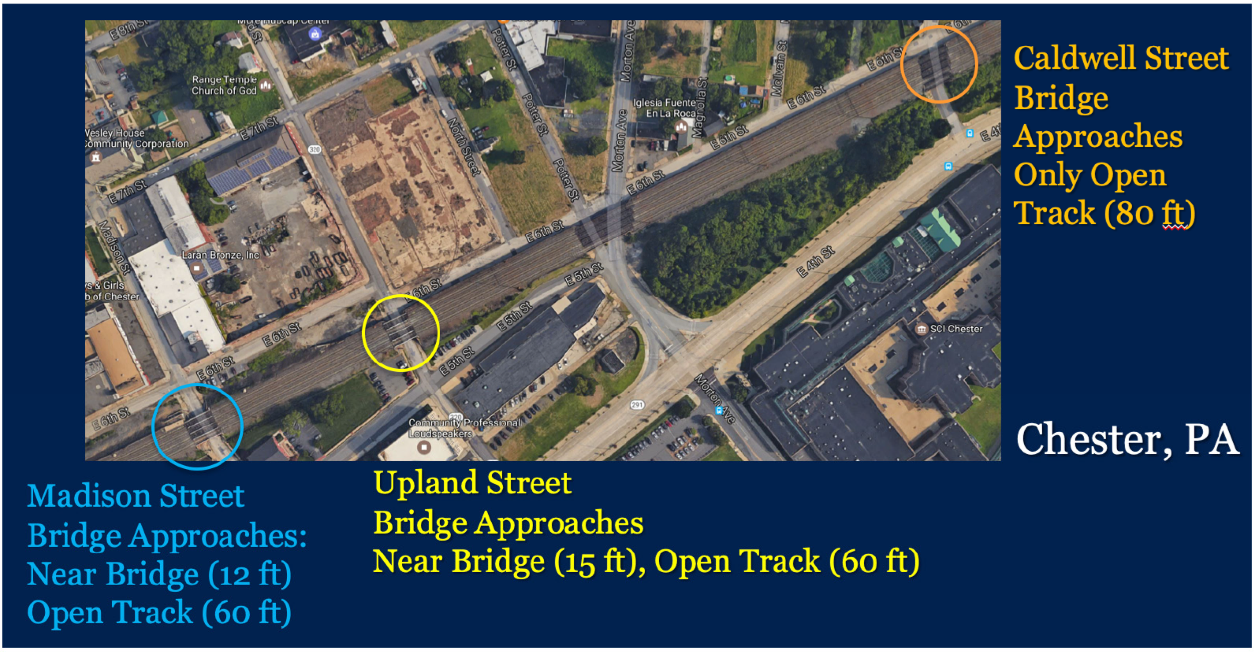
A problematic portion of Amtrak’s Northeast Corridor (NEC) was instrumented approximately 29 km (18 miles) south of Philadelphia near Chester, Pennsylvania. The instrumented sites comprise 8 to 10 closely spaced bridges with recurring differential movement issues at the bridge-embankment transitions. The NEC is primarily a high-speed passenger railroad with occasional freight traffic. On the NEC, the high-speed ACELA Express passenger train operates up to a maximum speed of 241 km/h (150 mph). This segment of NEC near Chester compromised a total of four tracks. Two of the tracks are maintained for high-speed passenger trains, typically operating at 177 km/h (110 mph). The current research focused on monitoring the track response and performance data due to ACELA passenger trains operating on the 2nd and 3rd main lines.

Historical track geometry data were obtained from Amtrak spanning a 60-month period from January 2005 to January 2010. In June of 2012, ground penetrating radar (GPR) scanning along the track was conducted to identify substructure features. The analyses of track geometry data and GPR data led to identifying the three worst bridge approach locations in terms of recurring differential movements. These are the open-deck bridges over Upland, Madison, and Caldwell Streets. These three locations with frequent maintenance needs were then selected in a US DOT Federal Railroad Administration supported project for field instrumentation, as shown in Figure 1 [27,28,29,30,31].

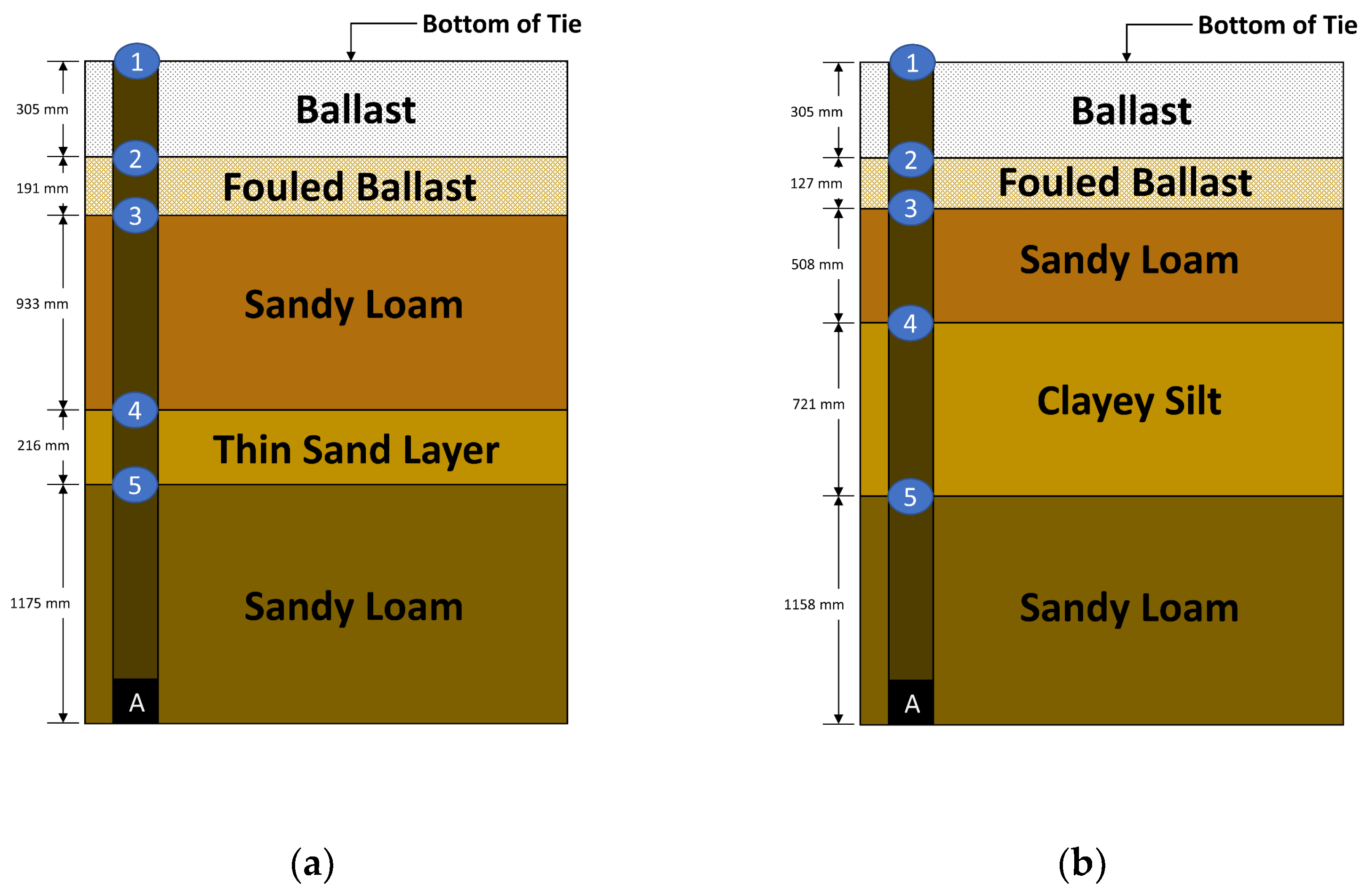
The instrumentation of Amtrak NEC bridge approaches took place in July-August of 2012. Multi-depth Deflectometers (MDDs) were selected to install and monitor the movement of individual track substructure layers. MDDs typically consist of several linear variable differential transformers (LVDTs) installed vertically at preselected depths to measure the displacements of individual substructure layers with respect to a fixed anchor buried deep in the ground [22,23,24,25,26]. Figure 2 shows the track substructure layer types and thicknesses encountered at the Upland Street instrumentation location.

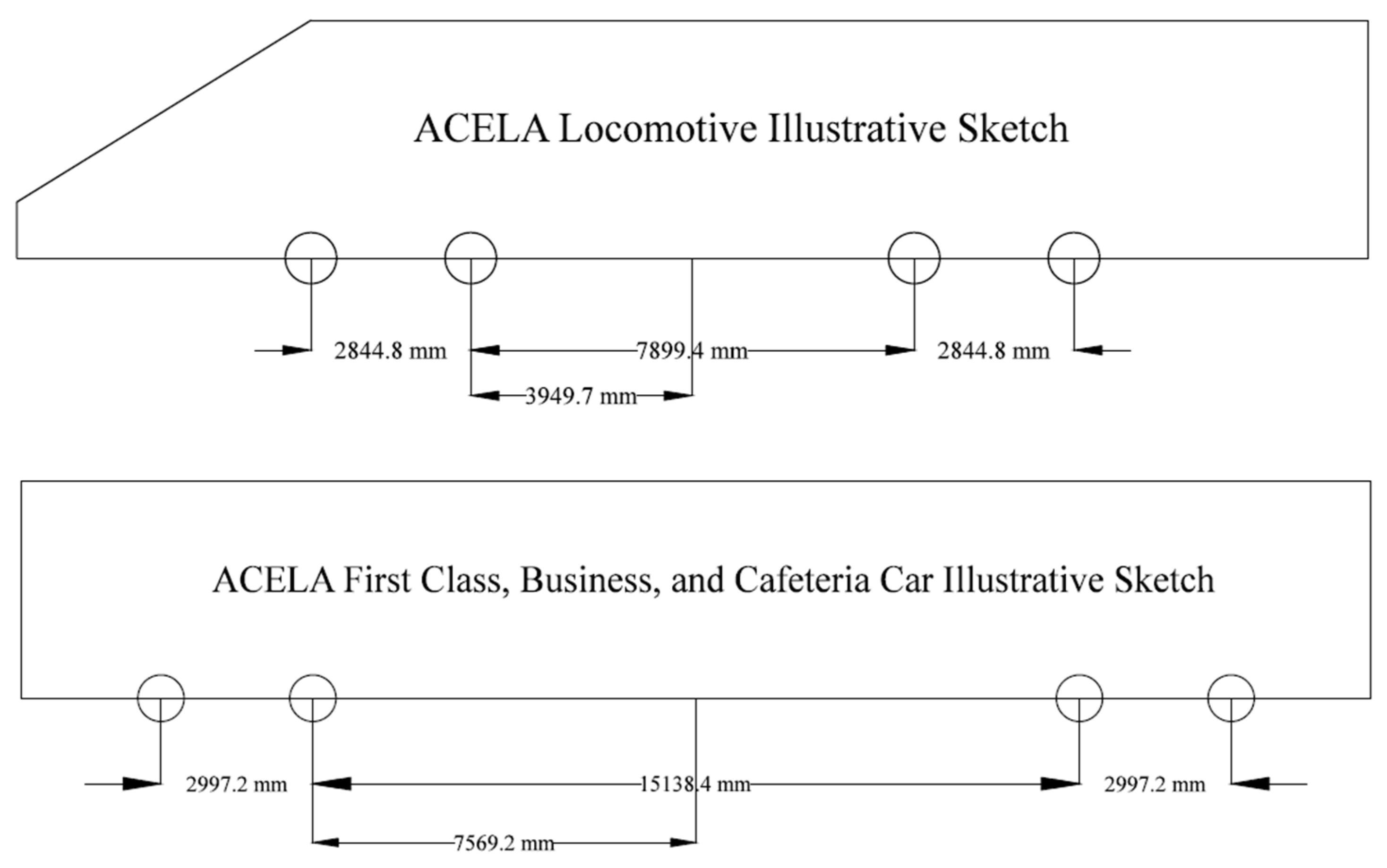
At the instrumented Amtrak NEC bridge approaches, the predominant train traffic is Acela Express passenger trains, operating at speed of 177 km/h (110 mph). An ACELA Express train consists of two locomotives, one at each end of the train, and six passenger cars in the middle. Figure 3 shows the bogie, axle, and wheel spacings for the Acela Express trains. As shown in the figure, the wheel spacing for Acela locomotive is approximately 2.8 m (110.2 in.); and the wheel spacing for Acela passenger car is approximately 3.0 m (118.1 in.).

2.2. Analyses of Field Data at Bridge Approaches

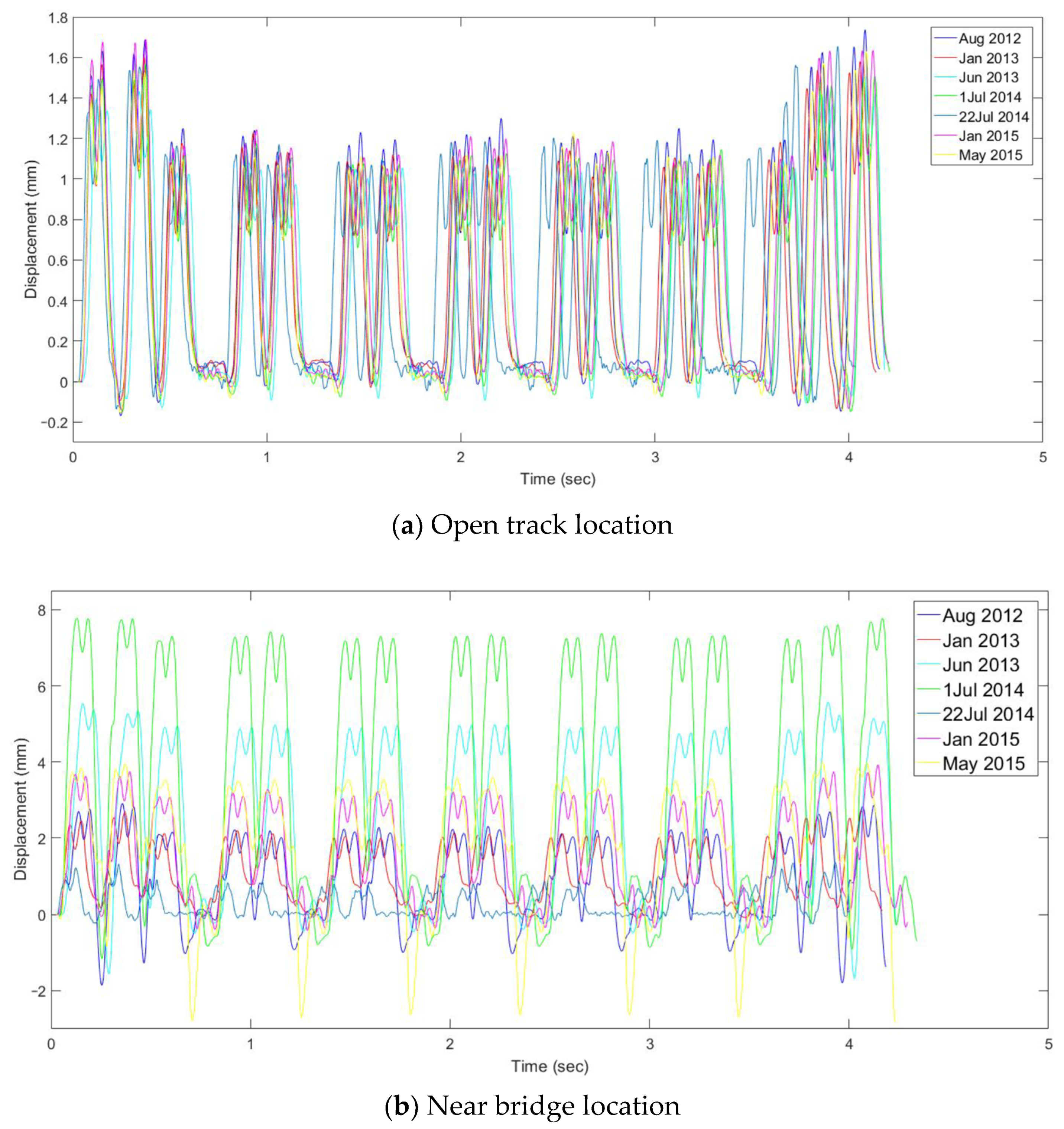
Figure 4 shows the transient vertical deformation time history recorded by LVDT modules under a passing train at open track location, which is 18.3 m (60 ft.) from abutment, and near bridge location, which is 4.6 m (15 ft.) from abutment. The recorded deformations corresponded to the eight-car ACELA Express passenger train, including one locomotive at each end of the train and six regular passenger cars. A total of 32 peaks were observed from the time history. These peaks corresponding to the passage of each wheel over the instrumented tie are quite distinguishable. Note that the locomotives created higher deformations compared to passenger cars since locomotives are heavier in weight. Moreover, it is important to note that at the open track location, the transient responses collected at different times are similar in magnitude. The maximum vertical transient deformation registered under ACELA Express train was approximately 1.7 mm.

It is important to note that unlike the open track data, the near bridge data showed great variability in magnitudes of transient deformations collected over time. The maximum vertical deformation continued to increase from August 2012 (2.5 mm) to 1 July 2014 (8 mm). Next, the maximum vertical deformation suddenly decreased to 1.6 mm on 22 July 2014, then up to 4 mm in May 2015. This sudden decrease in deformation was due to tamping maintenance activity conducted at the Upland Street location. In addition, a clear trend of increasing dynamic response was observed with time at the near bridge location. From visual inspection, it is noticeable that open track and near bridge locations have significantly different response trends under train passage.

From Figure 5, the peak transient deformation under locomotive passage at the open track location is nearly constant from 2012 until 2015. On the contrary, the peak deformation under locomotive passage at the near bridge location is changing drastically over time, and thus the deviation is larger, leading to a larger range for confidence interval. The statistics of the field data, including mean, standard deviation and 95% CI, of the peak transient deformation at both locations are summarized in

Table 1. Statistics of upland peak vertical transient deformations (2012–2015).

	Open Track (mm)	Near Bridge (mm)
Mean	1.63	4.03
Standard Deviation	0.07	2.10
95% CI High End	1.71	5.98
95% CI Low End	1.55	2.09

. Based on the statistical analysis, it is concluded that the vertical deformation behavior at the near bridge and open track locations are statistically different because the mean of one location does not fall within the 95% confidence interval of the other location. This implies the difference in dynamic responses at these two locations was not due to random error.

Large movements at the bridge approach will lead to accelerated track geometry degradation. Therefore, it is necessary to investigate the mechanism of the critical problem encountered at railroad track bridge approaches. This study is going to develop a train-track-bridge model at the bridge approach that can realistically predict responses under dynamic train loadings. Note that the January 2015 data were taken as an example in the following validation section to illustrate the large displacements at near bridge and contrast the trends between open track and near bridge locations.

3. Development of a Train-Track-Bridge Model

3.1. Physical Model and Parameters

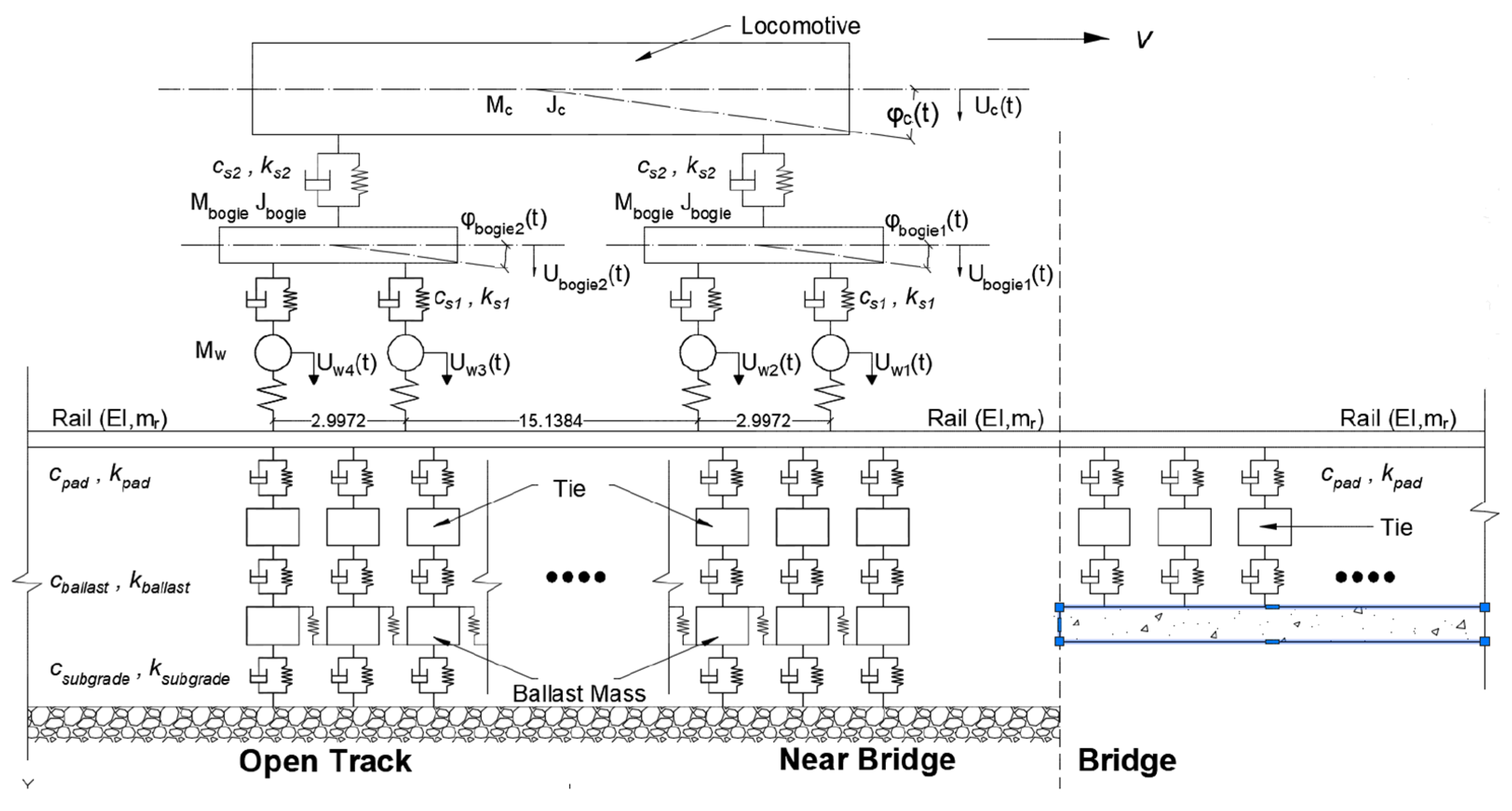
The train presented in the study consists of two locomotives at each end (front/rear) and six passenger cars in the middle, similar to the Amtrak’s ACELA Express passenger train operating over the instrumented bridge approaches, where the field instrumented bridge is an open deck bridge (no ballast) and there are tie gaps observed at such bridge approaches. Figure 6 illustrates the key components of a newly proposed train-track-bridge model. The train is assumed to travel in the arrow direction at a constant speed of v.

Each vehicle consists of one car body, two bogies, and four wheelsets. Each component is assumed to be a nondeformable rigid body that only has vertical movement or pitch movement. Each vehicle is modeled as a 10-degree-of-freedom system, consisting of vehicle car body vertical displacement $U_c$, vehicle car body pitch motion ${\phi }_c$, vertical displacement of the $U_{bog}$ of the two bogie masses, pitch motion ${\phi }_{bog}$ of the two bogie masses, and vertical displacement $U_w$ of the four wheel masses. The vehicle body is connected to the bogies through secondary suspension springs ($k_{s2}$) and dampers ($c_{s2}$). The bogies are connected to the wheels through primary suspension springs ($k_{s1}$) and dampers ($c_{s1}$). The primary and secondary suspension systems of the train vehicle are assumed to be linear.

The track structure on the open-track side is modeled by representing the rail as an infinite Euler beam discretely supported by three layers of viscous-elastic springs and dampers, representing rail pads, ballast, and soil, and two layers of masses, representing crossties and ballast. Crossties and ballast masses are assumed to be rigid bodies. Note that this newly developed model accounts for shear interaction between ballast particles. On the other hand, the track structure on the bridge side is modeled with the rail as an infinite Euler beam discretely supported by two layers of viscous-elastic foundations representing crossties resting directly on top of bridge deck (open deck bridge). At each time step, the vertical displacement of rail, $U_r$, vertical displacement of crosstie, $U_t$, and vertical displacement of ballast masses, $U_b$, are the remaining unknowns in time domain in the track system. Note that ‘open track location’ refers to a location far from bridge abutment and is assumed to be unaffected by the discontinuity in transition zone; while “near bridge location” refers to a location that is close to bridge abutment and may develop transition problems.

To obtain realistic dynamic responses in the track system from the introduced train-track- bridge model, the model parameters as input properties need to be chosen with physical relevance and careful attention.

Table 2. Model parameters and Inputs for the Train-Track-Bridge Model.

Track Properties
$\mathit{E}$	Young’s modulus of rail	2.07 × 105/3.0023 × 107	MPa/psi
$\mathit{I}$	Second moment of area	3.9 × 107/452 × 10−3	mm4/ft4
${\mathit{m}}_{\mathit{r}}$	Rail mass per unit length	67.46/4.533 × 10−2	kg/m/kip/ft
${\mathit{c}}_{\mathit{p}}$	Rail pad damping ratio	124/8.5	kN.s/m/kip.s/ft
${\mathit{k}}_{\mathit{p}}$	Rail pad stiffness	7.80 × 104/5.3447 × 103	kN/m/kip/ft
${\mathit{m}}_{\mathit{t}}$	Crosstie mass	386/0.85	kg/kips
${\mathit{m}}_{\mathit{b}}$	Ballast mass	683/1.5	kg/kips
${\mathit{c}}_{\mathit{b}}$	Ballast damping ratio	82/5.62	kN.s/m/kip.s/ft
${\mathit{k}}_{\mathit{b}}$	Ballast stiffness	1.20 × 105/8.223 × 103	kN/m/kip/ft
${\mathit{t}}_{\mathit{s}}$	Ballast shear stiffness	7.80 × 103/534.47	kN/m/kip/ft
${\mathit{c}}_{\mathit{s}}$	Subgrade damping ratio	300/20.56	kN.s/m/kip.s/ft
${\mathit{k}}_{\mathit{s}}$	Subgrade stiffness	5.00 × 104/3.426 × 103	kN/m/kip/ft
${\mathit{U}}_{\mathit{r}}$	Rail displacement	-
${\mathit{U}}_{\mathit{t}}$	Crosstie displacement	-
${\mathit{U}}_{\mathit{b}}$	Ballast displacement	-
${\mathit{k}}_{\mathit{v}\mathit{r}}$	Vehicle-rail stiffness	1.53 × 106/1.048 × 105	kN/m/kip/ft
Vehicle Properties
${\mathit{M}}_{\mathit{c}}$	Car body mass	6.31 × 104/139.11	kg/kip
${\mathit{J}}_{\mathit{c}}$	Car body mass inertia	1.20 × 106/2.848 × 104	kg.m2/kip.ft2
${\mathit{\phi }}_{\mathit{c}}$	Car body pitch rotation	-
${\mathit{U}}_{\mathit{c}}$	Car body displacement	-
${\mathit{c}}_{\mathit{s}2}$	Secondary suspension damping	70/4.8	kN.s/m/kip.s/ft
${\mathit{k}}_{\mathit{s}2}$	Secondary suspension stiffness	5.30 × 103/363.2	kN/m/kip/ft
${\mathit{M}}_{\mathit{b}\mathit{o}\mathit{g}\mathit{i}\mathit{e}}$	Bogie mass	1.20 × 103/2.646	kg/kip
${\mathit{J}}_{\mathit{b}\mathit{o}\mathit{g}\mathit{i}\mathit{e}}$	Bogie mass inertia	760/18.04	kg.m2/kip.ft2
${\mathit{\phi }}_{\mathit{b}\mathit{o}\mathit{g}\mathit{i}\mathit{e}}$	Bogie pitch rotation	-
${\mathit{U}}_{\mathit{b}\mathit{o}\mathit{g}\mathit{i}\mathit{e}}$	Bogie displacement	-
${\mathit{c}}_{\mathit{s}1}$	Primary suspension damping	49/3.358	kN.s/m/kip.s/ft
${\mathit{k}}_{\mathit{s}1}$	Primary suspension stiffness	2.10 × 103/143.9	kN/m/kip/ft
${\mathit{m}}_{\mathit{w}}$	Wheel mass	1.20 × 103/2.646	kg/kip
${\mathit{U}}_{\mathit{w}}$	Wheel displacement	-
$\mathit{P}$	Wheel-rail interaction force	-
$\mathit{a}$	Bogie distance	5.37/17.62	m/ft
$\mathit{b}$	Wheel distance	1.42/4.66	m/ft

lists the model parameters and presents one set of representative property values which are common in other published studies. Some of the track properties, such as crosstie spacing and rail properties, are selected based on realistic values at instrumented bridge approach locations at Amtrak’s Northeast Corridor (NEC). The other track properties, such as spring stiffness and damping ratio are selected from a list of previously published studies which also established a three-layer track model [32]. Vehicle parameters such as train mass, bogie and wheel spacings are selected from Amtrak ACELA Express passenger train’s vehicle data documented in a research report published by Judge and coworkers [33].

3.2. Equations of Motion of the Track System

The model introduced in Figure 6 consists of three major components—train, track, and bridge. To solve for the component dynamic responses, equilibrium equations are derived for each component. Note that each individual vehicle is considered independent. Hence, one vehicle rather than the whole train (eight vehicles) will be taken as an example to derive equilibrium equations.

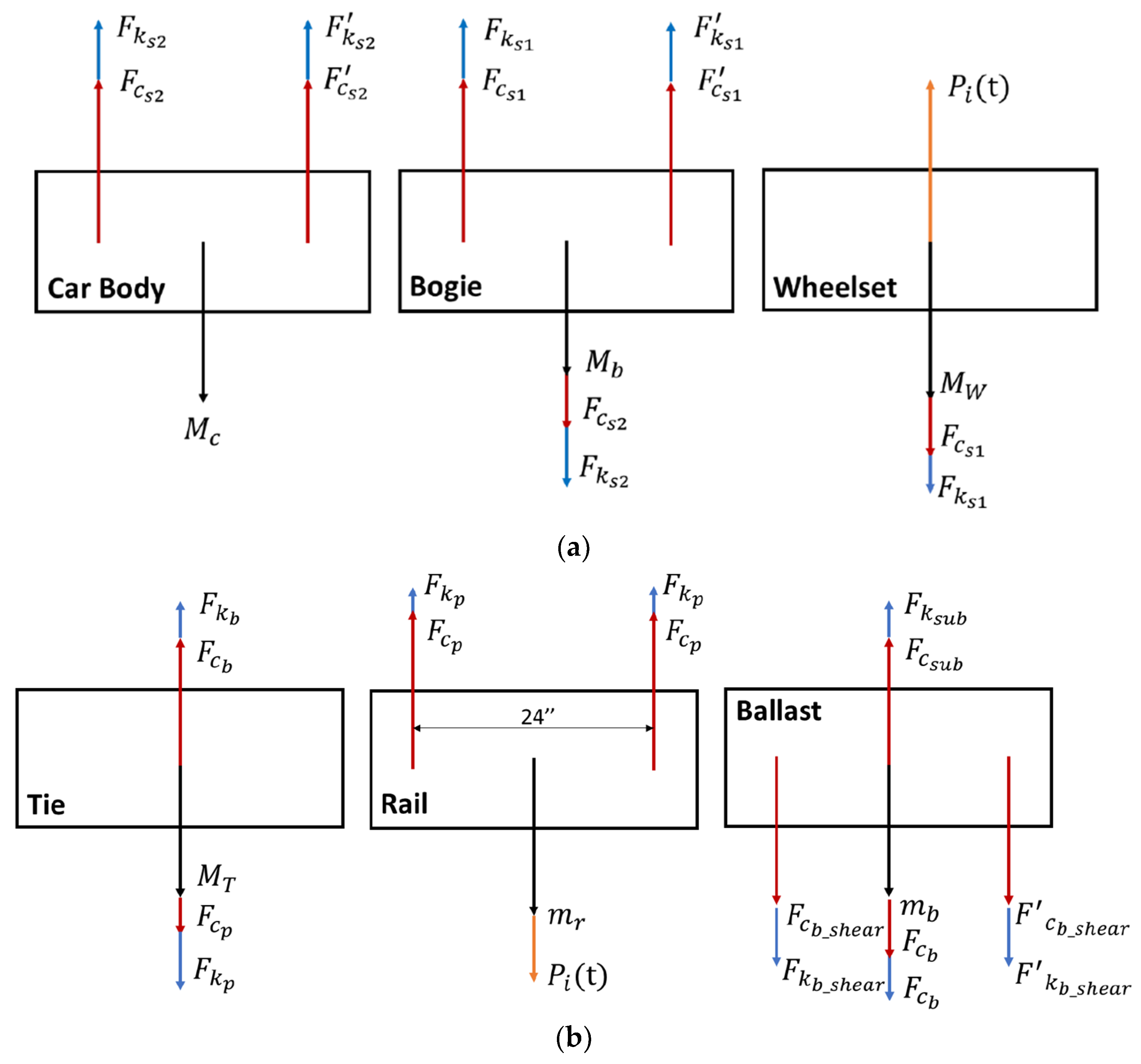
Only vertical transient displacement and pitch motion are considered for the vehicle. The body diagrams of dynamic force equilibrium for vehicle components are illustrated in Figure 7a. For example, the car body supported by two bogies reaches dynamic equilibrium with the external forces from bogies and self-weight. Similarly, each bogie is connected to the car body and two-wheel sets. The force equilibrium for the bogie is an equilibrium between self-weight of bogie, and contact forces between bogies and wheelsets, and contact forces between car body and bogie. Each wheel set has self-weight and two external forces, including contact force between wheelset and rail and contact force between wheelset and bogie. All the forces exerted on wheelset should reach equilibrium at any given time. Additionally, the equilibrium force, the equilibrium of moments for the bogie should also be achieved at the same time.

The unknown dynamic responses in the model, i.e., vertical displacement and pitch rotation angles, are in time domain. The system reaches both force and moment equilibrium at any given time, t, in the analysis period. The car body is connected to the bogies through secondary suspension springs with stiffness of $k_{s2}$ and dampers with damping ratio of $c_{s2}$, Equations (1) and (2) present the motion of car body. The bogies are connected to the wheels through primary suspension springs with stiffness of $k_{s1}$ and dampers with damping ratio of $c_{s1}$. Equations (3) and (4) give the motions of bogies, and Equation (5) presents the motion of wheels. The primary and secondary suspension systems of the train vehicle are assumed to be linear. Note that the notations used in following equations are defined in Table 1.

$$\begin{array}{c}{M}_c{\ddot{U}}_c+2c_{s2}{\dot{U}}_c+2k_{s2}{U}_c\\ -c_{s2}\left({\dot{U}}_{bogie1}+{\dot{U}}_{bogie2}\right)-k_{s2}\left(U_{bogie1}+U_{bogie2}\right)=M_{c}g\end{array}$$

(1)

$$\begin{array}{c}{J}_c{\ddot{\psi }}_c+2c_{s2}{a}^2{\dot{\psi }}_c+2k_{s2}{a}^2{\psi }_c\\ -c_{s2}a\left({\dot{U}}_{bogie1}+{\dot{U}}_{bogie2}\right)-K_{s2}a\left(U_{bogie1}-U_{bogie2}\right)=0\end{array}$$

(2)

$$\begin{array}{c}{M}_{bogie}{\ddot{U}}_{bogie1}+\left(c_{s2}+2c_{s1}\right){\dot{U}}_{bogie1}+\left(k_{s2}+2k_{s1}\right)U_{bogie1}\\ \mp c_{s2}\left({\dot{U}}_c+a{\dot{\psi }}_c\right)\mp k_{s2}\left(U_c+a{\psi }_c\right)\\ -c_{s1}\left({\dot{U}}_{w1}+{\dot{U}}_{w2}\right)-k_{s1}\left(U_{w1}+U_{w2}\right)=M_{bogie}g\end{array}$$

(3)

$$\begin{array}{c}{J}_c{\ddot{\psi }}_{bogie1}+2c_{s1}{b}^2{\dot{\psi }}_{bogie1}+2k_{s1}{b}^2{\psi }_{bogie1}\\ -c_{s1}b\left({\dot{U}}_{w1}-{\dot{U}}_{w2}\right)-k_{s1}b\left(U_{w1}-U_{w2}\right)=0\end{array}$$

(4)

$$\begin{array}{c}{M}_w{\ddot{U}}_{w1}+C_{s1}\left({\dot{U}}_{w1}-{\dot{U}}_{bogie1}\right)+k_{s1}\left(U_{w1}-U_{bogie1}\right)\\ -c_{s1}b{\dot{\psi }}_{bogie1}-k_{s1}b{\psi }_{bogie1}+P_i=M_{w}g\end{array}$$

(5)

where $M_c$, $M_{bogie}$, and $M_w$ are the masses of the car body, a bogie and a wheel, respectively. Contact force $P_i$ between wheel $i$ and the track is simulated by a linear spring connecting the two components, as indicated in Equation (6), where the magnitude of constant contact stiffness, $k_{vr}$, is selected from the Yu and Mao’s stochastic dynamic model [34]. Their model established a 3D train-track-bridge coupled system with refined wheel-rail interaction:

$$\begin{array}{c}{P}_i=k_{vr}\left(U_r-U_{wi}\right)\end{array}$$

(6)

Figure 7b shows the free body diagrams of track structure components. Crosstie comes to equilibrium under contact forces between rail and tie, contact forces between tie and ballast, and self-weight. A portion of the rail is taken as an example to illustrate the forces exerted on it, including vertical supports from underneath crosstie and vertical wheel loads from one wheelset running on top of that portion of the rail. Ballast particles experience a combination of shear forces between adjacent ballast particles, contact forces between ballast and subgrade, contact forces between ballast and crosstie, and self-weight.

In the train-track-bridge model formulation, the rail is supported by discrete crossties on top of the ballast layer from the track embankment side. The rail is modeled as an infinite Euler beam. The crossties are modeled as rigid masses at a spacing of 0.61 m (2 ft.) The ballast layer is modeled as rigid masses at the same crosstie spacing of 0.61 m (2 ft.). At the track embankment side (open track location), it is assumed that all the stiffnesses are linear. Therefore, the rail, crossties, and ballast masses in the model are connected with linear springs and dampers. Similar to the train component, the track structure components including rail, crossties, and ballast masses also exhibit force equilibrium at any given time t. The motions of rail beam, tie and ballast are given by Equations (7)–(9). The rail-tie reaction force, tie-ballast reaction force, and the shear force between ballast masses are calculated by Equations (10)–(12), respectively:

$$\begin{array}{c}EI\frac{{\partial }^4{U}_r\left(x,t\right)}{\partial x^4}+{\rho }_r\frac{{\partial }^2{U}_r\left(x,t\right)}{\partial t^2}+{\displaystyle \sum _1^M}{a}_m\left(t\right)\delta \left(x-x_m\right)\\ ={\displaystyle \sum _{i=1}^4}{P}_i\delta \left(x-vt-x_i\right)\end{array}$$

(7)

$$m_t\frac{{\partial }^2{U}_t\left(x_m,t\right)}{\partial t^2}=a_m\left(t\right)-b_m\left(t\right)$$

(8)

$$\begin{array}{c}{m}_b\frac{{\partial }^2{U}_b\left(x_m,t\right)}{\partial t^2}=b_m\left(t\right)\\ -c_s\frac{\partial U_b\left(x_m,t\right)}{\partial t}-k_s{U}_b\left(x_m,t\right)+T_m-T_{m+1}\end{array}$$

(9)

$$\begin{array}{c}{a}_m\left(t\right)=c_p\left(\frac{\partial U_r\left(x_m,t\right)}{\partial t}-\frac{\partial U_t\left(x_m,t\right)}{\partial t}\right)\\ +k_p\left(U_r\left(x_m,t\right)-U_t\left(x_m,t\right)\right)\end{array}$$

(10)

$$\begin{array}{c}{b}_m\left(t\right)=c_b\left(\frac{\partial U_t\left(x_m,t\right)}{\partial t}-\frac{\partial U_b\left(x_m,t\right)}{\partial t}\right)\\ +k_b\left(U_t\left(x_m,t\right)-U_b\left(x_m,t\right)\right)\end{array}$$

(11)

$$T_m=t_s\left(U_b\left(x_{m-1},t\right)-U_b\left(x_m,t\right)\right)$$

(12)

Similar to the open track embankment side, the rail is also modeled as an infinite Euler beam for the bridge side (the Euler beam is extending from open track side to the bridge side). In addition, since the field instrumented bridge is an open deck bridge without ballast, ballast layer is not considered on bridge deck in the train-track-bridge model. Therefore, on the bridge side in the model, the rail is supported by discrete crossties directly sitting on top of a rigid bridge deck. The crossties are modeled as rigid masses at a spacing of 0.61 m (2 ft.) between each crosstie. At first, since no hanging ties are considered, the rail, crossties, and nondeformable bridge deck are assumed to be connected by linear springs and dampers. The bridge deck is assumed non-deformable, which is an approximation for bridge abutment in the field. Realistically, if the bridge deck has a long span, it would undergo large deformation under dynamic loading. However, the proposed model focuses on the dynamic responses at open track location and near bridge location. Therefore, the bridge deck behavior is simplified. The track structure components including rail and crossties reach the state of force equilibrium at any given time, t. The motion of its rail beam and tie can be calculated in a similar manner using Equations (13) and (14). Its rail-tie reaction forces can be calculated using Equation (15):

$$\begin{array}{c}EI\frac{{\partial }^4{U}_r\left(x,t\right)}{\partial x^4}+{\rho }_r\frac{{\partial }^2{U}_r\left(x,t\right)}{\partial t^2}+{\displaystyle \sum _{M+1}^M}{a}_m\left(t\right)\delta \left(x-x_m\right)\\ ={\displaystyle \sum _{i=1}^4}{P}_i\delta \left(x-vt-x_i\right)\end{array}$$

(13)

$$m_t\frac{{\partial }^2{U}_t}{\partial t^2}=a_m\left(t\right)-k{U}_t\left(x_m,t\right)-c\frac{\partial U_t\left(x_m,t\right)}{\partial t}$$

(14)

$$\begin{array}{c}{a}_m\left(t\right)=c_p\left(\frac{\partial U_r\left(x_m,t\right)}{\partial t}-\frac{\partial U_t\left(x_m,t\right)}{\partial t}\right)\\ +k_p\left(U_r\left(x_m,t\right)-U_t\left(x_m,t\right)\right)\end{array}$$

(15)

3.3. Coupling of Track Structure and Train

The equations of motion for vehicle components, crossties and ballast masses listed in Equations (16)–(18), respectively, are all used to assemble the final matrix. To be concise, one car of the train, consisting of one car body, two bogies, and four wheelsets, were considered here to illustrate the basic form of the final matrix.

$$\left[M_v\right]\left\{{\ddot{U}}_v\right\}+\left[C_v\right]\left\{{\dot{U}}_v\right\}+\left[K_v\right]\left\{U_v\right\}=\left\{F_v\right\}$$

(16)

$$\begin{array}{c}\left[M_2\right]\left\{{\ddot{U}}_t\right\}+\left[C_3\right]\left\{\dot{q}\right\}+\left[K_3\right]\left\{q\right\}+\left[C_4\right]\dot{\left\{U_t\right\}}+\left[K_4\right]\left\{U_t\right\}\\ +\left[C_5\right]\dot{\left\{U_b\right\}}+\left[K_5\right]\left\{U_b\right\}=\left\{0\right\}\end{array}$$

(17)

$$\left\{{\ddot{U}}_b\right\}+\left[C_6\right]\left\{{\dot{U}}_b\right\}+\left[K_b\right]\left\{U_b\right\}+\left[C_7\right]\dot{\left\{U_t\right\}}+\left[K_7\right]\left\{U_t\right\}=\left\{0\right\}$$

(18)

In solving all the above equations, the general equations of motion in standard matrix form is presented in Equation (19), consisting of generalized mass, damping, stiffness matrices, and force vector. Note that $\left\{X\right\}$ denotes the generalized displacement vector containing displacement of car body, bogies, wheelsets, rail, crossties, and ballast masses, as well as the pitch angle of car body and bogies at any given time t; $\left[M\right]$ denotes the generalized mass matrix; $\left[C\right]$ denotes the generalized damping matrix; $\left[K\right]$ denotes the generalized stiffness matrix; and $\left\{F\right\}$ denotes the generalized force vector.

$$\left[M\right]\left\{\ddot{X}\right\}+\left[C\right]\left\{\dot{X}\right\}+\left[K\right]\left\{X\right\}=\left\{F\right\}$$

(19)

3.4. Numerical Integration Using Newmark’s Method

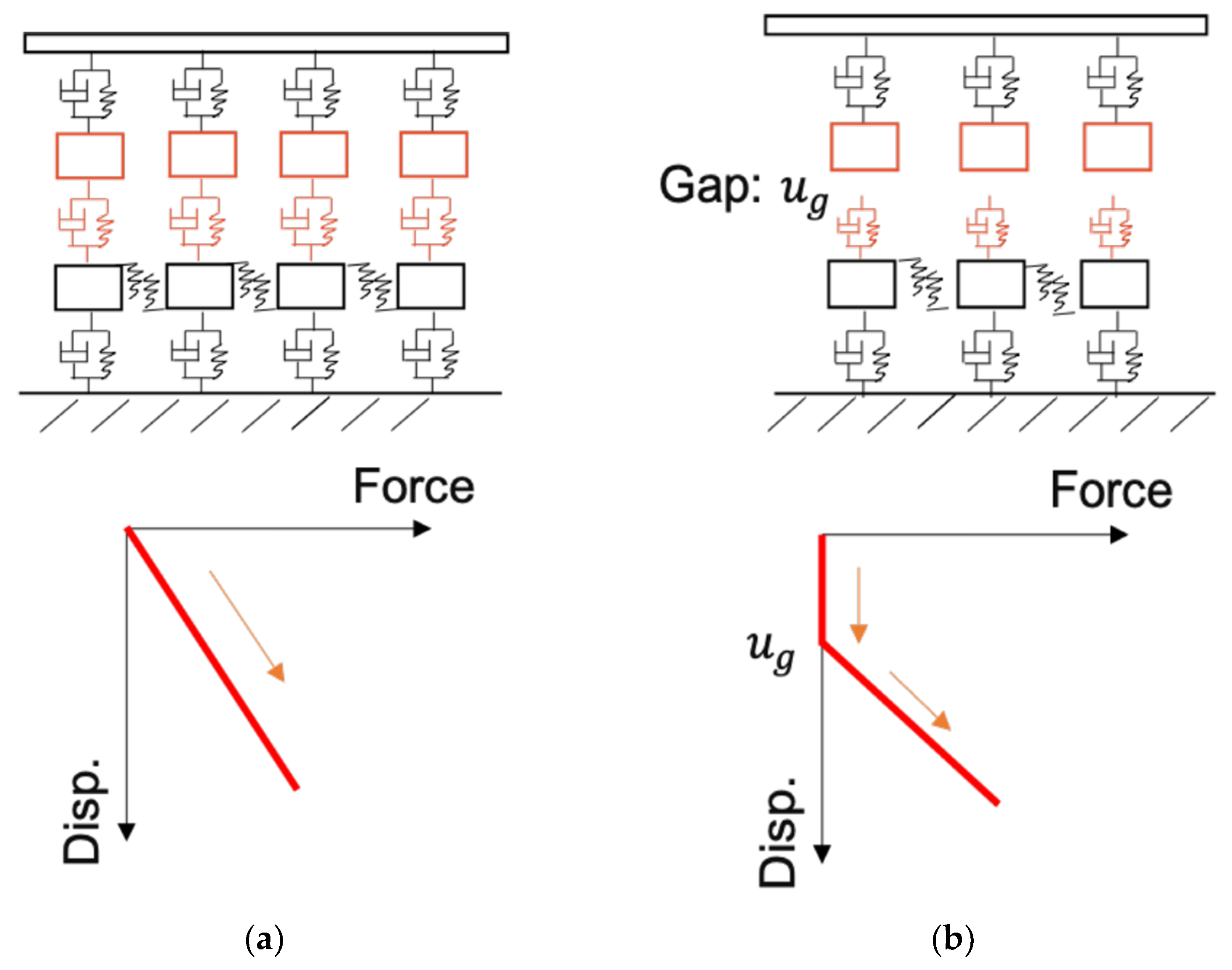
Hanging crossties exist very often at track near bridge locations. These hanging crossties commonly lack adequate support from the ballast layer underneath it. Figure 8 presents schematics showing the model structure with and without gaps, as well as the corresponding force-displacement relations. For these inadequately supported crossties, the force-displacement relationship cannot be assumed to be linear elastic anymore. Instead, it becomes nonlinear due to the gap between the tie and ballast. For simplicity, the proposed nonlinear train-track-bridge model assumes bi-linear force-displacement relationship. More specifically, it is assumed that at the beginning of loading, there is no force between the crosstie and ballast until the gap ($u_g$) is closed. Once the distance between the crosstie and ballast reaches the magnitude of gap, the stiffness of springs between the crosstie and ballast becomes linear ($k{\prime }_{ballast}$). Note that the tangent of stiffness from open track and near bridge locations might be different, i.e., $k_{ballast}\ne k{\prime }_{ballast}$. It is assumed that damping coefficient, $c{\prime }_{ballast}$, at near bridge is constant in the analysis. Figure 8 illustrates the force-displacement relationship at (a) open track location with linear stiffness and (b) near bridge location with nonlinear stiffness. The gap between crosstie and ballast is represented by $u_g$. Note that in the model, the locations of the gap will not affect the results since it is discretely supported. The amount of gap underneath each crosstie can also be assigned arbitrarily based on realistic situations.

Numerical integration method can be utilized to solve the generalized matrix, but the generalized stiffness matrix needs to be updated in each iteration to simulate the effect of moving vehicle because the location of vehicle-rail contact force, $P_i$, is changing. There are several widely used numerical integration methods for solving the generalized matrix. For instance, Fourier transformation is one method to solve linear equations of motion. However, one disadvantage of the Fourier transformation method is that it is restricted to linear systems. A system is considered nonlinear when damping or stiffness properties vary in time. In this situation, the calculation of the response of a nonlinear system can be done only by a step-by-step direct integration. In the track-bed system, the suspension system between crossties and ballast particles can be nonlinear if the crossties are not properly supported. Direct time integration method is applicable to both linear and nonlinear systems. Hence, it is a general method to calculate response of dynamic system under arbitrary loading. Many methods exist for the direct integration of the equations of motion. Herein, Newmark’s method has been chosen to solve the equations of motion in the track bed system. Newmark’s method, also called Newmark-β method, was developed by Nathan Newmark for use in structural dynamics, based on finite difference method [35].

Table 3. Algorithm for numerical integration using Newmark’s method for nonlinear (or bilinear) systems.

Initialization of The Variables
Initial condition	${\mathit{u}}_{\mathit{0}}\mathit{=}\mathit{0}\mathit{,}\dot{{\mathit{u}}_{\mathit{0}}}\mathit{=}\mathit{0}\mathit{,}{\mathit{p}}_{\mathit{0}}\mathit{=}\mathit{0},{\mathit{t}}_{\mathit{0}}\mathit{=}\mathit{0}$
Calculation initial condition	${\ddot{u}}_0=\left(p_0-c\dot{u_0}-k{u}_0\right)\mathbf{/}\mathit{m}$
Average acceleration method	$\mathit{\gamma }\mathbf{=}\mathbf{0.5}\mathbf{,}\mathit{\beta }\mathbf{=}\mathbf{0.25}$
Integration time step	$\Delta \mathit{t}\mathbf{=}\mathbf{0.001}$
Preliminary Calculations
Calculate the integration constants	${\mathit{a}}_{\mathbf{0}}\mathbf{=}\frac{1}{\mathit{\beta }\mathbf{\Delta }{\mathit{t}}^{\mathbf{2}}}\mathbf{;}{\mathit{a}}_{\mathbf{1}}\mathbf{=}\frac{\mathit{\gamma }}{\mathit{\beta }\mathbf{\Delta }\mathit{t}}\mathbf{;}{\mathit{a}}_{\mathbf{2}}\mathbf{=}\frac{\mathbf{1}}{\mathit{\beta }\mathbf{\Delta }\mathit{t}}\mathbf{;}{\mathit{a}}_{\mathbf{3}}\mathbf{=}\frac{\mathbf{1}}{\mathbf{2}\mathit{\beta }}\mathbf{;}{\mathit{a}}_{\mathbf{4}}\mathbf{=}\frac{\mathit{\gamma }}{\mathit{\beta }}\mathbf{;}{\mathit{a}}_{\mathbf{5}}\mathbf{=}\mathbf{\left(}\frac{\mathit{\gamma }}{\mathbf{2}\mathit{\beta }}\mathbf{-}\mathbf{1}\mathbf{\right)}\mathbf{\Delta }\mathit{t}$
Integrate Step by Step for$\mathit{n}\mathbf{=}\mathbf{0}\mathbf{,}\mathbf{1}\mathbf{,}\mathbf{2}\mathbf{,}\mathbf{\dots }\mathbf{,}\frac{{\mathit{t}}_{\mathit{d}}}{\mathbf{\Delta }\mathit{t}}$:
Increment time	${\mathit{t}}_{\mathit{n}\mathbf{+}\mathbf{1}}\mathbf{=}{\mathit{t}}_{\mathit{n}}\mathbf{+}\mathbf{\Delta }\mathit{t}\mathbf{=}\mathbf{\left(}\mathit{n}\mathbf{+}\mathbf{1}\mathbf{\right)}\mathbf{\Delta }\mathit{t}$
Calculate effective tangent stiffness	${\widehat{\mathit{K}}}_{\mathit{n}}\mathbf{=}{\mathit{K}}_{\mathit{n}}\mathbf{+}{\mathit{a}}_{\mathbf{0}}\mathit{M}\mathbf{+}{\mathit{a}}_{\mathbf{1}}\mathit{C}$, if tie gap closes
Calculate increment of the effective force $\mathbf{\Delta }\widehat{\mathit{p}}$ at time ${\mathit{t}}_{\mathit{n}}$	$\mathbf{\Delta }\widehat{\mathit{p}}\mathbf{=}\mathit{p}\mathbf{+}\mathbf{\left(}{\mathit{a}}_{\mathbf{2}}{\dot{\mathit{u}}}_{\mathit{n}}\mathbf{+}{\mathit{a}}_{\mathbf{3}}{\ddot{\mathit{u}}}_{\mathit{n}}\mathbf{\right)}\mathit{M}\mathbf{+}\mathbf{\left(}{\mathit{a}}_{\mathbf{4}}{\dot{\mathit{u}}}_{\mathit{n}}\mathbf{+}{\mathit{a}}_{\mathbf{5}}{\ddot{\mathit{u}}}_{\mathit{n}}\mathbf{\right)}\mathit{C}$
Calculate increment of displacement $\mathbf{\Delta }\mathit{u}$	$\mathbf{\Delta }\mathit{u}\mathbf{=}\frac{\mathbf{\Delta }\widehat{\mathit{p}}}{{\widehat{\mathit{K}}}_{\mathit{n}}}$
Calculate increment of velocity $\mathbf{\Delta }\dot{\mathit{u}}$	$\mathbf{\Delta }\dot{\mathit{u}}\mathbf{=}{\mathit{a}}_{\mathbf{1}}\mathbf{\Delta }\mathit{u}\mathbf{-}{\mathit{a}}_{\mathbf{4}}\dot{{\mathit{u}}_{\mathit{n}}}\mathbf{-}{\mathit{a}}_{\mathbf{5}}{\ddot{\mathit{u}}}_{\mathit{n}}$
Calculate displacement and velocity at time ${\mathit{t}}_{\mathit{n}\mathbf{+}\mathbf{1}}$	${\mathit{u}}_{\mathit{n}\mathbf{+}\mathbf{1}}\mathbf{=}{\mathit{u}}_{\mathit{n}}\mathbf{+}\mathbf{\Delta }\mathit{u}\mathbf{,}{\dot{\mathit{u}}}_{\mathit{n}\mathbf{+}\mathbf{1}}\mathbf{=}{\dot{\mathit{u}}}_{\mathit{n}}\mathbf{+}\mathbf{\Delta }\dot{\mathit{u}}$
Calculate acceleration at time ${\mathit{t}}_{\mathit{n}\mathbf{+}\mathbf{1}}$	${\ddot{\mathit{u}}}_{\mathit{n}\mathbf{+}\mathbf{1}}\mathbf{=}({\mathit{p}}_{\mathit{n}\mathbf{+}\mathbf{1}}\mathbf{-}\mathit{c}{\dot{\mathit{u}}}_{\mathit{n}\mathbf{+}\mathbf{1}}\mathbf{-}{\mathit{f}}_{\mathit{n}\mathbf{+}\mathbf{1}})\mathbf{/}\mathit{m}$

illustrates the initialization and integration steps in the algorithm. Average acceleration method is utilized with parameters γ = 0.5, and β = 0.25. This method is unconditionally stable and is always converging in the end. Therefore, no time step restriction applies. The time step of Δt = 0.001 can be selected in this case to account for a compromised accurate loading function and computational time. The initial conditions are assumed at stationary.

4. Model Validation with Field Collected Data

4.1. Model Validation for Open Track Location

The ACELA Express passenger train operates at a speed of 177 km/h (110 mph) at the Upland Street location in Chester, PA, USA. The passenger car weight is approximately 618.3 kN (139 kips). Transient deformation data with train passage were collected in the field at two locations: (1) The open track location which is 18.3 m (60 ft.) from the bridge abutment and (2) the near bridge location, which is 4.6 m (15 ft.) from the bridge abutment. The January 2015 data were taken as an example to illustrate the large displacements at near bridge and contrast the trends between the open track and near bridge locations. Such large movements at the bridge approach will lead to accelerated degradation of the track geometry.

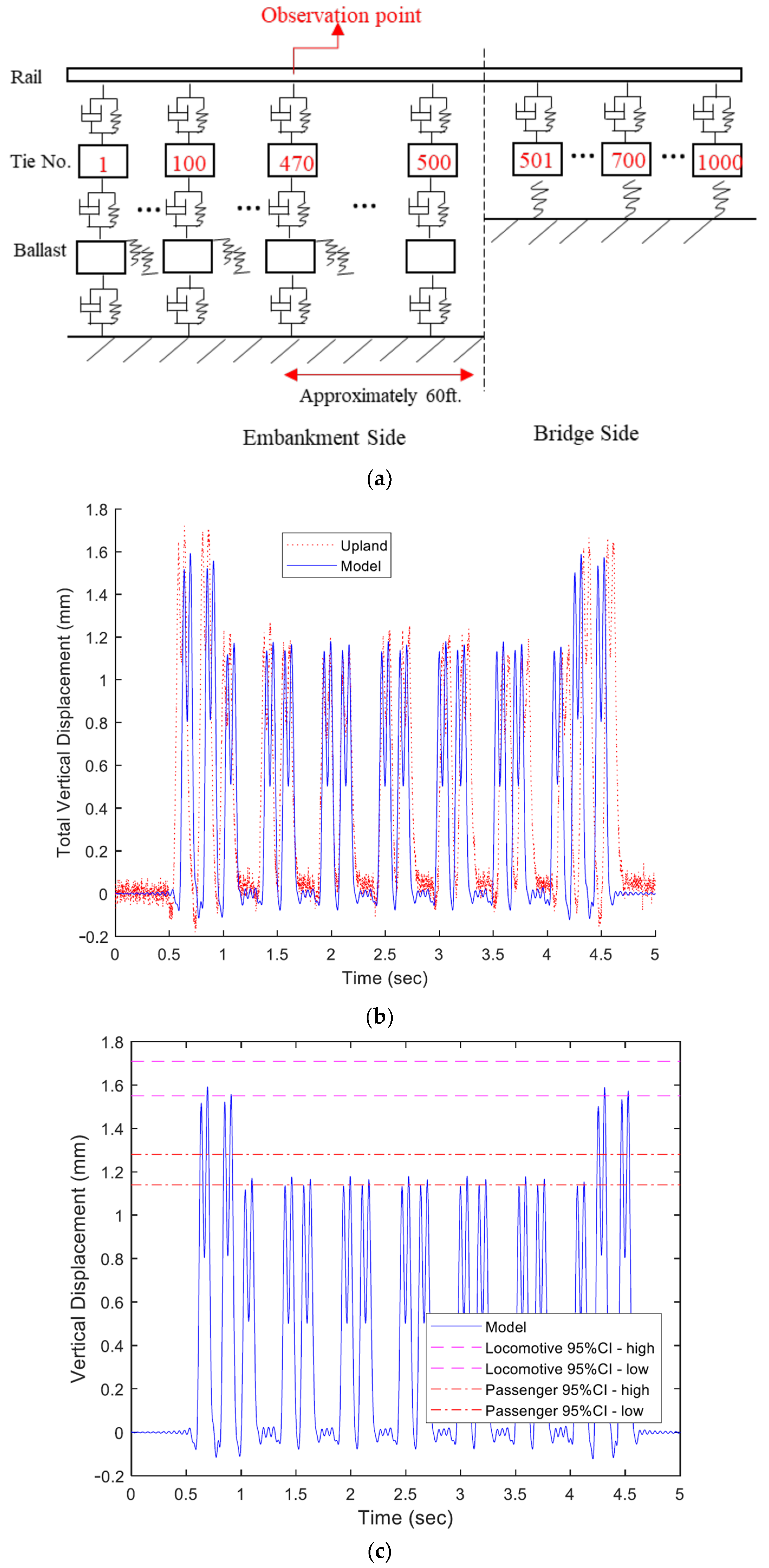
To eliminate the boundary effect of vehicles entering and leaving the track structure, the number of crossties on the embankment side is assumed to be 500 and the number of crossties on the bridge side is also assumed to be 500. Crossties are located at a spacing of 0.61 m (2 ft.). In the field open track location, the data were collected at 18.3 m (60 ft.) from the bridge abutment, approximately 30 crossties away from the bridge deck. Figure 9a illustrates the corresponding observation point in the model.

According to the vehicle properties in Table 2, the locomotive in this case consisted of one car body, two bogies and four wheels, representing the weight of car as 880.8 kN (198 kips). The passenger car consists of one car body, two bogies, and four wheels, representing the weight of car as 618.3 kN (139 kips). The vehicle is moving at a speed of 177 km/h (110 mph). The flexural rigidity of rail beam is 8.073 $\mathrm{MN}·{\mathrm{m}}^2$ (19,535.21 $\mathrm{kips}·{\mathrm{ft}}^2$).

With the ACELA Express passenger train moving from embankment side to bridge side in the model, the structural responses including transient deformation, reaction force, velocity, and acceleration can be obtained from the model. Field collected data are then used to validate the transient deformations obtained from the numerical model. Figure 9b,c show the comparisons between model predictions and field data. Figure 9b clearly shows that the results from the proposed model match well with the field data collected in January 2015. The model simulation results demonstrate 32 peaks, which correspond to 8 cars with one passage of ACELA passenger train. The front and rear of the train register higher displacements due to heavier weights of the locomotives. Figure 9c compares the confidence intervals of field data and model predictions. The maximum peak displacement predicted by the model falls into the 95% confidence interval calculated from the maximum peak displacement value from the field data collected between August 2012 and May 2015.

4.2. Model Validation for Near Bridge Location

To validate the model predictions with the near bridge location field data, the model input parameters were kept the same as those for the open track location except for the observation point in the model, and realistically considering that the hanging crosstie gap induced nonlinear stiffness assignment. Accordingly, at the field instrumented near bridge location, data were collected at 4.6 m (15 ft.) from the bridge abutment, approximately 7 to 8 crossties away from the bridge deck. Therefore, crosstie no. 493 was chosen as the observation point in the model as shown in Figure 10a. The time history of structural responses at the observation point were then calculated to simulate dynamic response behavior of the track structure at the near bridge location.

In addition to the changing of observation point, nonlinear ballast stiffness representing hanging crossties should also be properly simulated. Hanging crossties were observed in the field at the near bridge location, where there were gaps between these hanging crossties and the underlying ballast particles. At the instrumented Upland Street location, the gap was found to increase over time when the track lacked proper maintenance. For calibration and validation purposes, a typical gap of 1.5 mm (0.005 ft.) (developed in January 2013) was selected in the model simulation. Such gaps were created underneath crossties no. 485 to no. 500 in the model. Before the gap closes, it is assumed that no force exists between crosstie and ballast mass. As soon as the gap fully closes during the loading process, the ballast stiffness abruptly increases to a similar value as that for open track locations −120 $\mathrm{MN}/{\mathrm{m}}^2$ (2506.3 $\mathrm{kips}/{\mathrm{ft}}^2$). For simplicity, it is assumed that the ballast damping ratio remains constant at the near bridge location.

To validate the track model, transient deformations predicted by the model simulations are compared to the field measured transient deformations. Figure 10b,c show the comparisons between the model predictions and the field data. The model simulation results clearly demonstrate 32 peaks, which correspond to 8 cars with one passage of ACELA passenger train. The front and rear of the train register slightly higher displacements due to heavier weights of the locomotives. Due to the existence of a tie gap, the peak displacement of a moving locomotive can be as high as 2.6 mm (0.0085 ft.). If the gap continues to increase, it is anticipated that the transient deformation can reach a significantly high value at the near bridge location.

Figure 10b shows that the general trends of transient deformations in terms of peak location and peak magnitude under loading are comparable with the field data. However, the deformations predicted between wheel axles do not match very well with the field measured data. The physical meaning of this “delayed bouncing” is that in the simplified physical relationship between displacement and force for hanging crossties, there is little reaction force when the differential movement between crosstie and ballast mass is small (k~0). Hence, there is not sufficient upward direction force exerted on crosstie for the bounce back movement. In contrast, the fastening system will lead the crosstie to move back to its original position in the field, even though there is no upward force from the underlying ballast.

Figure 10c compares the confidence intervals of field data collected in January 2013 and model results. The upper and lower boundaries of 95% confidence intervals are graphed for locomotive passage and passenger car passage, respectively. Due to the increase in the gap amount with time, the peak displacement may vary significantly. Therefore, the higher and lower boundaries of the confidence intervals are relatively far away from each other compared with the open track scenario. It is noticed that the maximum peak displacement value from the model still falls into the 95% confidence interval calculated from the maximum peak displacement value from the field data collected between August 2012 and May 2015.

The proposed model is thus capable of predicting the general trends and peak responses, but not the bouncing movement. Considering that the main purpose of the model is to detect the critical responses, it is believed that the proposed model has been successfully validated with field measurements at the near bridge location.

5. Train Induced Track Structure Response Predictions

The comparisons between the field data and model results imply that responses at the open track and the near bridge locations could be accurately predicted and simulated by the developed train-track-bridge model. Therefore, the validated train-track-bridge model can be utilized to analyze other critical responses under the train passage.

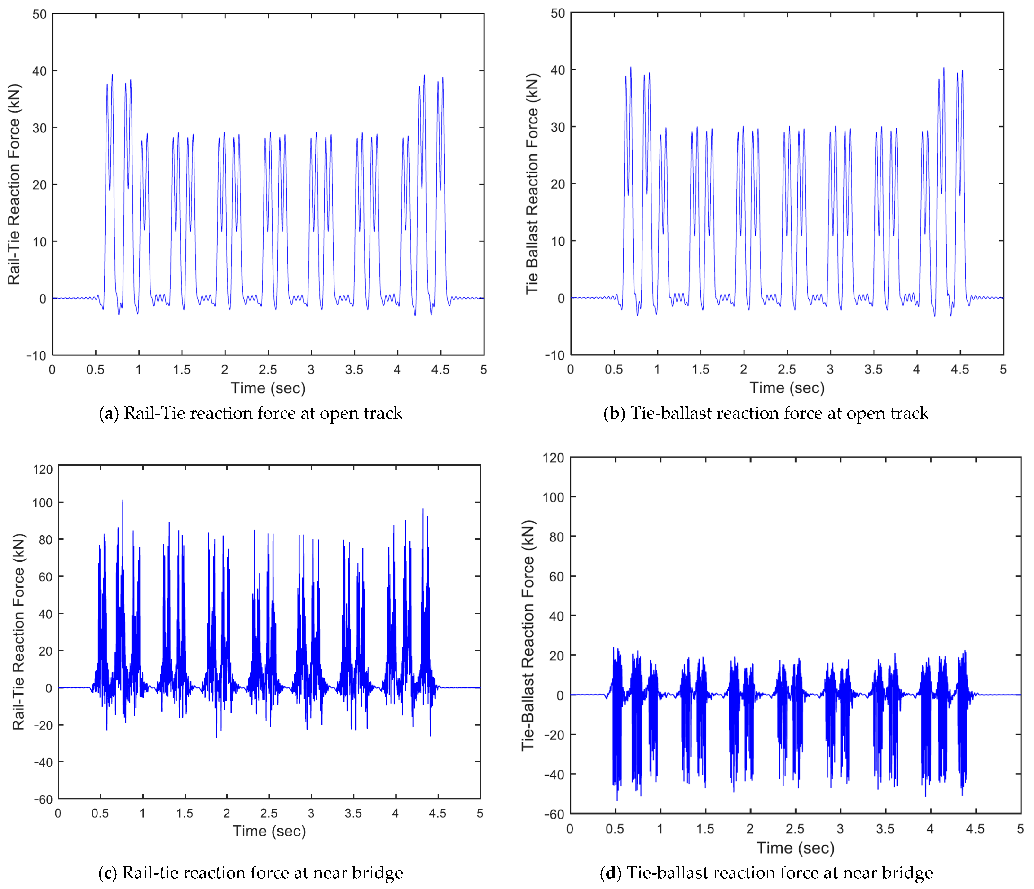
5.1. Reaction Forces

The graphs shown in Figure 11 present the rail-crosstie reaction force and crosstie-ballast reaction force with train passage at the open track and near bridge locations. Note that the rail-crosstie reaction force and crosstie-ballast reaction force at the open track location are similar in both trends and magnitudes (see Figure 11a,b). This confirms that the force is correctly simulated in the model since at the open track location the crossties are in good contact with the underlying ballast particles and, thus, the external force exerted on crossties can be adequately passed on to the ballast mass. According to the field data, the average measured wheel load on rail crib in the field at the open track location is around 132 kN (29.7 kips) for a locomotive and 91 kN (20.5 kips) for a passenger car. In the track model simulation, the crosstie reaction force is approximately 40 kN (9 kips) for a locomotive and 29 kN (6.52 kips) for a passenger car. Hence, it is found that each crosstie takes up to 30–32% of the train wheel load. However, the nonlinear model at the near bridge location registers more “noise” when compared to the open track location. From the field measured data, the average peak wheel load on rail crib due to locomotive pass is approximately 148 kN and the average peak wheel load on rail crib due to passenger car pass is approximately 100 kN. From the model predictions, the peak rail-crosstie reaction forces corresponding to locomotive and passenger car are found to be around 100 kN and 80 kN, respectively. Even though the impact wheel load on crib is only slightly higher than that at the open track location, the reaction force on crossties takes up to 67–80% of the total impact force at the near bridge location compared with 30% of the total force at the open track location. Such high impact force would lead to accelerated degradation of both rail and crossties in the field.

In addition to the rail-tie reaction force, tie-ballast reaction force also exhibits quite different behavior as compared to the open track location. At the open track location, the rail-tie reaction and tie-ballast reaction forces are comparable in both trends and magnitude. However, at the near bridge location, it is noticed that the tie-ballast reaction force is considerably smaller than rail-tie reaction force (see Figure 11c,d). Such difference in rail-tie reaction force value and tie-ballast reaction force is the total external force on crosstie, causing possibly larger vibration accelerations.

5.2. Vibration Velocities and Accelerations

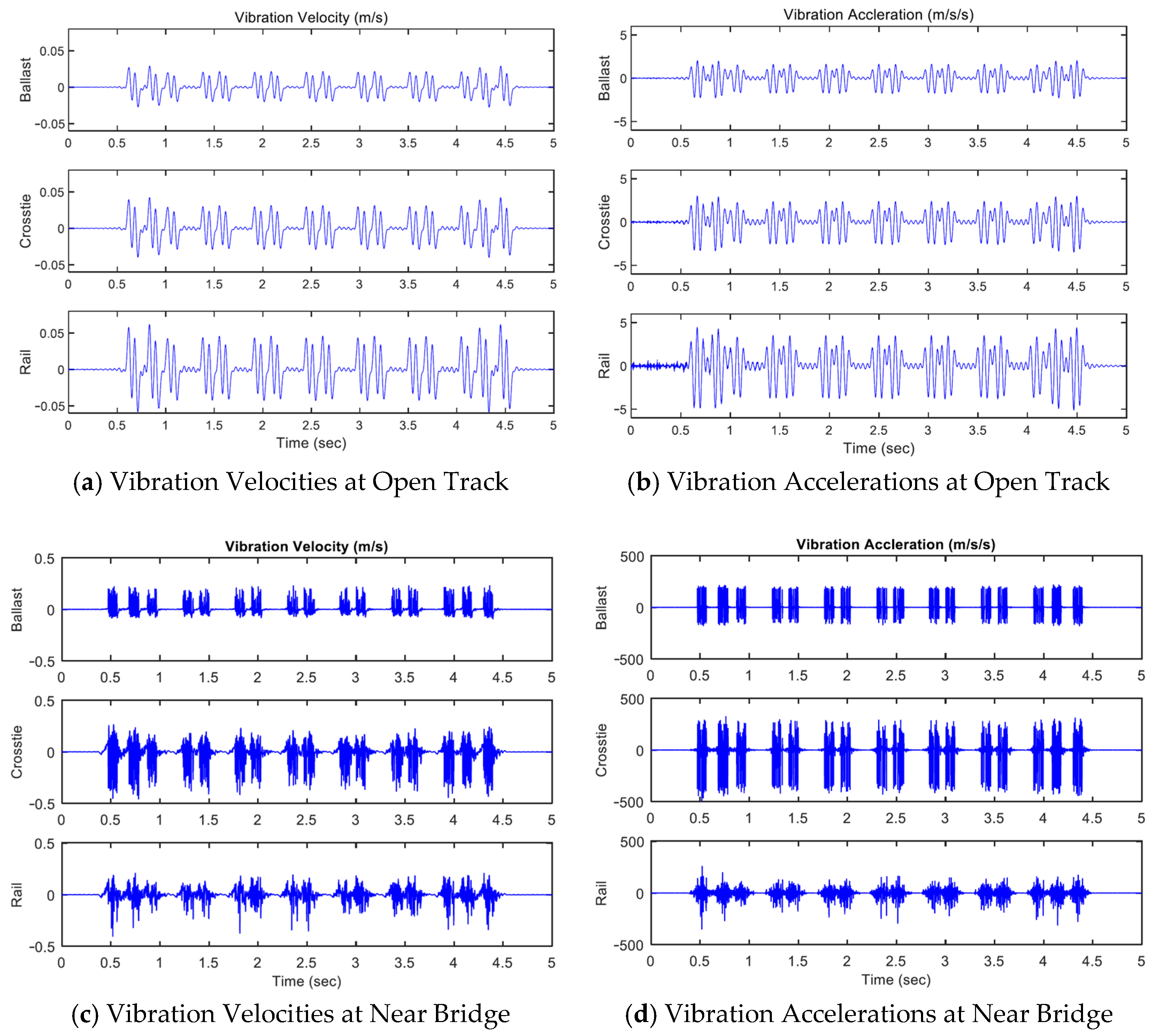
The structural vibration velocities and accelerations can also be predicted from the model simulations. Figure 12a shows the time history of vibration velocities of ballast mass, crosstie and rail, respectively. The peaks represent each wheelset of the ACELA Express passenger train. It is noticed that the vibration velocities of different components in the system have similar magnitude of 10⁻² m/s. Furthermore, ballast mass registers the lowest vibration velocity in the system of 0.027 m/s; crosstie mass shows slightly higher velocity of 0.039 m/s; and rail mass implies the highest velocity of 0.058 m/s. Similarly, the time history of vibration accelerations of the track system is graphed in Figure 12b. The vibration accelerations of different components are all below one standard gravitational acceleration, g = 9.8 $\mathrm{m}/{\mathrm{s}}^2$. The peak accelerations at the open track location are approximately 2 $\mathrm{m}/{\mathrm{s}}^2$ for ballast mass; 3 $\mathrm{m}/{\mathrm{s}}^2$ for crosstie, and 4.5 $\mathrm{m}/{\mathrm{s}}^2$ for rail mass.

From Figure 12c, the vibration velocities at the near bridge location are within the range of (−0.5 ~ +0.5) m/s;. The magnitude is almost ten times of that at the open track location. Larger vibration velocity majorly comes from inadequate support of the hanging crossties. Rail registers the smallest positive peak vibration velocity of 0.15 m/s. Ballast mass vibrates with a slightly higher velocity of 0.2 m/s. The peak vibration velocity of crosstie is approximately 0.26 m/s. Figure 12d clearly demonstrates that the track system accelerations at the near bridge location are significantly higher than those obtained at the open track location. The standard g = 9.8 m/s² is used as the measurement unit. Recall that the accelerations at the open track location are all below 1 g. While the accelerations at the near bridge location are all above 10 g. Peak vibration acceleration of rail is about 15 g under ACELA Express passenger train. Ballast masses experience larger accelerations under loading with a peak vibration acceleration of 20 g. And the crosstie exhibits the highest vibration acceleration of up to 40 g. Higher accelerations in the track system can lead to component degradation including ballast shakedown more easily. In conclusion, the track model prediction results imply greater risk of material degradation at the near bridge location.

6. Conclusions and Future Work

This paper aimed to develop a novel train-track-bridge model at the track transition zone of a bridge approach to effectively simulate the dynamic response and performance of track structure under moving train loads. The objective was to better understand governing mechanisms of bridge approach problems such as differential settlement and unsupported hanging ties that occur near bridge abutments by the use an analytical model. To develop the train-track-bridge model, Newmark’s numerical integration method was chosen to solve the set of ordinary differential equations for the track system because it can be applied to both linear system (open track location) and nonlinear system (near bridge location) with a ballast-tie gap. The force-displacement relationship between crossties and ballast masses at both open track and near bridge locations are also presented. The spring stiffness is assumed to be nonlinear at near bridge location. Accordingly, Newmark’s method was modified to evaluate the tangent stiffness at every step to solve for the nonlinear system within tolerable error.

The model predictions for transient displacements successfully matched with field measured data collected for both the open track and near bridge locations from a comprehensive instrumentation and field monitoring project that took place on Amtrak’s main passenger lines on the Northeast Corridor near Chester, Pennsylvania. This validated the developed train-track-bridge model. Hanging tie scenario at near bridge location could be simulated as a nonlinear spring between crosstie and ballast masses in the track model.

According to the analyses of field data, it is observed that the vertical wheel loads at near bridge locations were relatively constant and stable over the three years monitored, however, the transient deformations at near bridge locations showed clear increasing trends for the same monitoring period. This phenomenon indicates noticeable change in substructure support conditions over a relatively shorter time at the near bridge locations. Additionally, it is found that the transient deformation performance as well as loading on rail from the two locations were statistically different. Such major differences are not due to random error in data collection. There is a need to determine the physical mechanisms that govern at railroad track bridge approaches and contribute to the behavioral differences.

The model predictions clearly showed that near bridge location experienced larger vertical deformations, especially for crosstie; larger impact forces on rail, crosstie, and ballast layer; larger vibration velocities; and larger vibration accelerations. From the perspective of critical dynamic responses, it can be concluded that the difference between the largest displacements between open track and near bridge locations could be significant. Based on this study, the transient deformation at the near bridge location showed an increasing trend over the years, while the vertical wheel loads at near bridge location were relatively stable, indicating noticeable change in substructure support condition overtime. The model predictions indicated that at open track location, each crosstie takes approximate 30–32% of the train wheel load. In contrast, a crosstie may take up to 67% of the train wheel load at near bridge location.

It is important to note that rail irregularity was not considered in the developed train-track-bridge model, which could lead to an underestimation of the track system responses. The validated model is an analysis tool that may help to evaluate common remedial measures, including stone blowing, installation of under tie pads (UTPs) and polyurethane injection. Future studies are recommended to include rail irregularity and its effects on the predicted dynamic responses. Another important question concerns the development of a three-dimensional train-track-bridge model to include lateral forces and derailment potential analyses, and to consider tamping and other track maintenance schedules for maintaining proper track geometry. The purpose of this model is to stimulate how train travels through bridge approaches with unsupported hanging ties on straight tangent track; future studies can also take curved track into consideration. Moreover, it would be useful to collect field geometry data over a longer period of time and combine it with the numerical model for transient force and displacement field data collection. The combined permanent and transient deformation data can be analyzed using machine learning techniques to predict important indices of track structure, such as permanent deformation, derailment potential, and differential movements.

References

- Sañudo, R.; Dell’Olio, L.; Casado, J.A.; Carrascal, I.A.; Diego, S. Track transitions in railways: A review. Constr. Build. Mater. 2016, 112, 140–157. [Google Scholar] [CrossRef]
- Li, D.; Davis, D. Transition of railroad bridge approaches. J. Geotech. Eng. 2005, 131, 1392–1398. [Google Scholar] [CrossRef]
- Banimahd, M.; Woodward, P.K.; Kennedy, J.; Medero, G.M. Behavior of train–track interaction in stiffness transitions. In Proceedings of the Institution of Civil Engineers-Transport; Thomas Telford Ltd.: London, UK, 2012; Volume 165, pp. 205–214. [Google Scholar]
- Basu, D.; Rao, N.S.V.K. Analytical solutions for Euler–Bernoulli beam on viscoelastic foundation subjected to moving load. Int. J. Numer. Anal. Methods Geomech. 2013, 37, 945–960. [Google Scholar] [CrossRef]
- Bian, X.; Chen, Y.; Hu, T. Numerical simulation of high-speed train induced ground vibrations using 2.5 D finite element approach. Sci. China Ser. G Phys. Mech. Astron. 2018, 51, 632–650. [Google Scholar] [CrossRef]
- Cheli, F.; Corradi, R. On rail vehicle vibrations induced by track unevenness: Analysis of the excitation mechanism. J. Sound Vib. 2011, 330, 3744–3765. [Google Scholar] [CrossRef]
- Huang, H.; Gao, Y.; Stoffels, S. Fully coupled three-dimensional train-track-soil model for high-speed rail. Transp. Res. Rec. J. Transp. Res. Board 2014, 2448, 87–93. [Google Scholar] [CrossRef]
- Li, X.; Ekh, M.; Nielsen, J. Three-dimensional modelling of differential railway track settlement using a cycle domain constitutive model. Int. J. Numer. Anal. Methods Geomech. 2016, 40, 1758–1770. [Google Scholar] [CrossRef]
- Ling, L.; Xiao, X.; Xiong, J.; Zhou, L.; Wen, Z.; Jin, X. A 3D model for coupling dynamics analysis of high-speed train/track system. J. Zhejiang Univ. Sci. A 2014, 15, 964–983. [Google Scholar] [CrossRef] [Green Version]
- Sharma, R.C.; Sharma, N.; Sharma, S.; Sharma, S.K. Analysis of generalized force and its influence on ride and stability of railway vehicle. Noise Vib. Worldw. 2020, 51, 95–109. [Google Scholar] [CrossRef]
- Koziak, S.; Chudzikiewicz, A.; Opala, M.; Melnik, R. Virtual software testing and certification of railway vehicle from the point of view of their dynamics. Transp. Res. Procedia 2019, 40, 729–736. [Google Scholar] [CrossRef]
- Coelho, B.; Priest, J.; Holscher, P.; Powrie, W. Monitoring of Transition Zones in Railways; Engineering Technics Press: Oxford, UK, 2009. [Google Scholar]
- Zhai, W.; Xia, H.; Cai, C.; Gao, M.; Li, X.; Guo, X.; Wang, K. High-speed train– track–bridge dynamic interactions–Part I: Theoretical model and numerical simulation. Int. J. Rail Transp. 2013, 1, 3–24. [Google Scholar] [CrossRef]
- Varandas, J.N.; Hölscher, P.; Silva, M.A. Dynamic behavior of railway tracks on transitions zones. Comput. Struct. 2011, 89, 1468–1479. [Google Scholar] [CrossRef]
- Varandas, J. Long-Term Behavior of Railway Transitions under Dynamic Loading. Ph.D. Thesis, Faculdade de Cieˆncias e Tecnologia da Universidade Nova de Lisboa, Almada, Portugal, 2013. [Google Scholar]
- Yang, C.; Sun, H.; Zhang, J. Dynamic responses of bridge-approach embankment transition section of HSR. J. Cent. South Univ. 2013, 20, 2830–2839. [Google Scholar] [CrossRef]
- Indraratna, B.; Sajjad, M.; Ngo, T.; Gomes Correia, A.; Kelly, R. Improved performance of ballasted tracks at transition zones: A review of experimental and modelling approaches. Transp. Geotech. 2019, 21, 100260. [Google Scholar] [CrossRef]
- Czyczula, W.; Koziol, P.; Blaszkiewicz, D. On the Equivalence between Static and Dynamic Railway Track Response and on the Euler-Bernoulli and Timoshenko Beams Analogy. Shock Vib. 2017, 2017, 1–13. [Google Scholar] [CrossRef] [Green Version]
- Wang, H.; Markine, V. Methodology for the comprehensive analysis of railway transition zones. Comput. Geotech. 2018, 99, 64–79. [Google Scholar] [CrossRef]
- Wang, H.; Markine, V. Dynamic behavior of the track in transitions zones considering the differential settlement. J. Sound Vib. 2019, 459, 114863. [Google Scholar] [CrossRef]
- Kaewunruen, S.; Remennikov, A.; Aikawa, A. A numerical study to evaluate dynamic responses of voided concrete railway sleepers to impact loading. In Proceedings of the Australian Acoustical Society Conference 2011, Acoustics 2011: Breaking New Ground, Gold Coast, Australia, 2–4 November 2011; pp. 464–471. [Google Scholar]
- Giner, I.; López Pita, A.; Vieira Chaves, E.; Rivas Álvarez, A. Design of embankment–structure transitions for railway infrastructure. In Proceedings of the Institution of Civil Engineers-Transport; Thomas Telford Ltd.: London, UK, 2012; Volume 165, pp. 27–37. [Google Scholar]
- Wang, H.; Markine, V.L.; Shevtsov, I.Y.; Dollevoet, R. Analysis of the dynamic behavior of a railway track in transition zones with differential settlement. In 2015 Joint Rail Conference; American Society of Mechanical Engineers: New York, NY, USA, 2015. [Google Scholar]
- Yin, C.; Wei, B. Numerical simulation of a bridge-subgrade transition zone due to moving vehicle in Shuohuang heavy haul railway. J. Vibroeng. 2013, 15, 1041–1047. [Google Scholar]
- Wu, Y.; Yang, Y. Steady-state response and riding comfort of trains moving over a series of simply supported bridges. Eng. Struct. 2003, 25, 251–265. [Google Scholar] [CrossRef]
- Rakoczy, A.M.; Shu, X.; Duane, O. Vehicle–track–bridge interaction modeling and validation for short span railway bridges. Transp. Res. Rec. 2017, 2642, 127–138. [Google Scholar] [CrossRef]
- Mishra, D.; Tutumluer, E.; Boler, H.; Hyslip, J.; Sussmann, T. Railroad track transitions with multidepth deflectometers and strain gauges. Transp. Res. Rec. J. Transp. Res. Board 2014, 2448, 105–114. [Google Scholar] [CrossRef]
- Mishra, D.; Boler, H.; Tutumluer, E.; Hyslip, J.P. Effectiveness of Chemical Grouting and Stone Blowing as Remedial Measures to Mitigate Differential Movement at Railroad Track Transitions. In 2016 Joint Rail Conference; American Society of Mechanical Engineers: New York, NY, USA, 2016. [Google Scholar]
- Tutumluer, E.; Stark, T.D.; Mishra, D.; Hyslip, J.P. Investigation and mitigation of differential movement at railway transitions for US high speed passenger rail and joint passenger/freight corridors. In 2012 Joint Rail Conference; American Society of Mechanical Engineers: New York, NY, USA, 2012; pp. 75–84. [Google Scholar]
- Mishra, D.; Tutumluer, E.; Stark, T.D.; Hyslip, J.P.; Chrismer, S.M.; Tomas, M. Investigation of differential movement at railroad bridge approaches through geotechnical instrumentation. J. Zhejiang Univ. Sci. A 2012, 13, 814–824. [Google Scholar] [CrossRef]
- Tutumluer, E.; Mishra, D.; Boler, H.; Hyslip, J.P.; Thomas, M. Dynamic Responses of Bridge Approach Concrete Ties after the Applications of Polyurethane Injection, Stone Blowing and Under-Tie Pad Remedial Measures. In International Crosstie and Fastening System Symposium. June 2016. Available online: https://railtec.illinois.edu/wp/wp-content/uploads/pdf-archive/9.2_Tutumluer.pdf (accessed on June 2019).
- Cantero, D.; Arvidsson, T.; OBrien, E.; Karoumi, R. Train–track–bridge modelling and review of parameters. Struct. Infrastruct. Eng. 2016, 12, 1051–1064. [Google Scholar] [CrossRef]
- Judge, A.; Ho, C.; Huang, H.; Hyslip, J.; Gao, Y. Field Investigation and Modeling of Track Substructure Performance Under Trains Moving at Critical Speed. 2018. Available online: https://railroads.dot.gov/elibrary/field-investigation-and-modeling-track-substructure-performance-under-trains-moving (accessed on June 2019).
- Yu, Z.W.; Mao, J.F. A stochastic dynamic model of train-track-bridge coupled system based on probability density evolution method. Appl. Math. Model. 2018, 59, 205–232. [Google Scholar] [CrossRef]
- Newmark, N.M. A Method of Computation for Structural Dynamics; Department of Civil Engineering, University of Illinois: Champaign, IL, USA, 1959. [Google Scholar]
Figure 1.
Locations of the Three Bridges Selected for Instrumentation in Amtrak’s NEC (1 ft = 30.5 cm).
Figure 2.
Substructure Layer Profile for (a) Upland Street 4.6 m (15 ft.) from the North Abutment; and (b) Upland Street 18.3 m (60 ft.) from the North Abutment.
Figure 3.
ACELA locomotive and passenger car axle spacings.
Figure 4.
Transient vertical deformations with train passage at Upland.
Figure 5.
Upland peak vertical transient deformations over time (2012–2015).
Figure 6.
Train-Track-Bridge Model developed at the University of Illinois.
Figure 7.
Free Body Diagrams for (a) vehicle components and (b) track components.
Figure 8.
Linear and nonlinear dynamic systems: (a) Linear stiffness at open track location, and (b) nonlinear stiffness at near bridge location.
Figure 9.
Open track location—(a) Sketch of response observation point in the model; and (b) comparisons of model predictions and field data.
Figure 10.
Near Bridge Location: (a) Sketch of the response observation point in the model; and (b) comparisons of model predictions and field data.
Figure 11.
Model predicted reaction forces with ACELA Express passenger train passage.
Figure 12.
Model predicted structural vibration velocities and accelerations with ACELA Express passenger train passage.