
Railway Track Loss-of-Stiffness Detection Using Bogie Filtered Displacement Data Measured on a Passing Train

 ,
,  , and
, and
Abstract
:1. Introduction
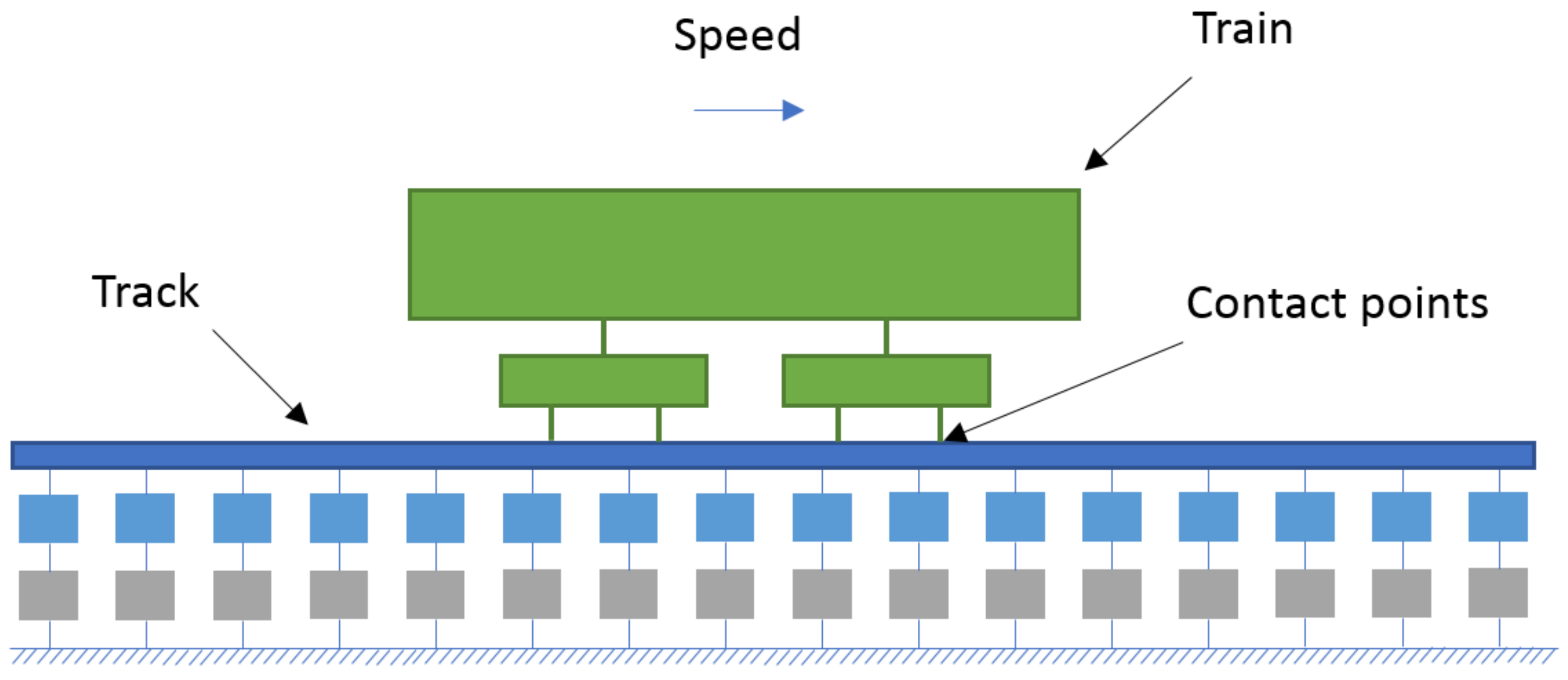
2. Numerical Modeling of Track Train Interaction
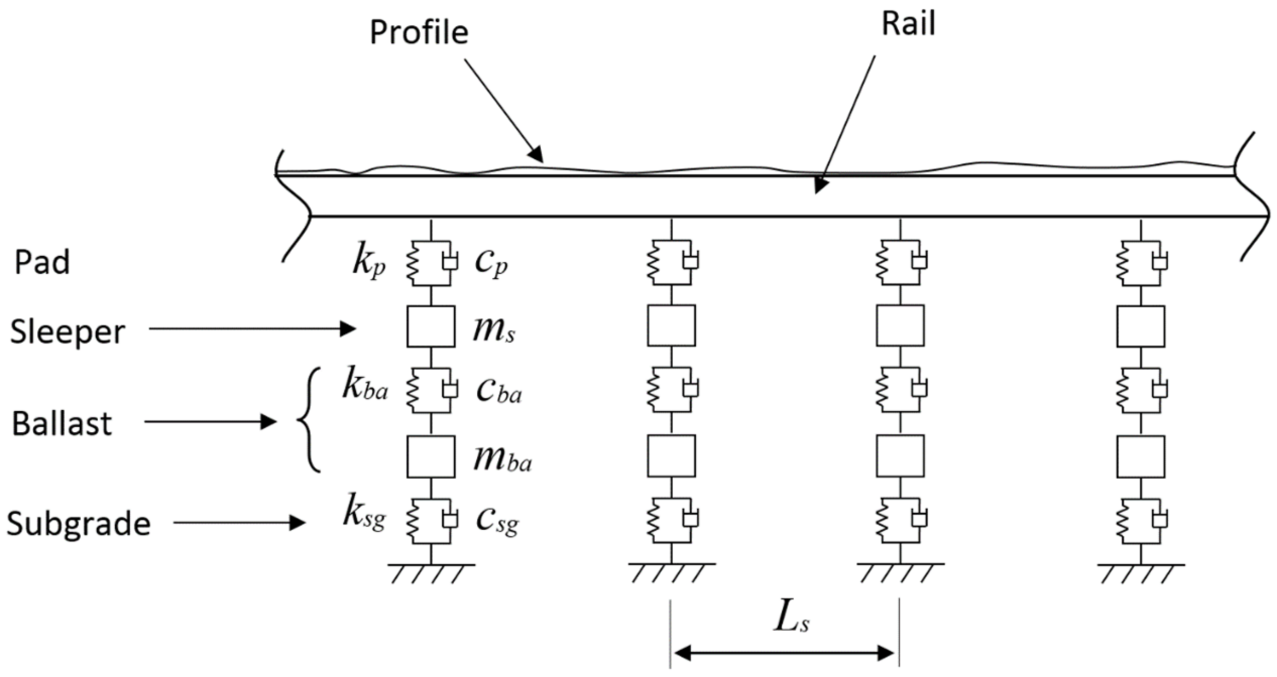
2.1. Track Model
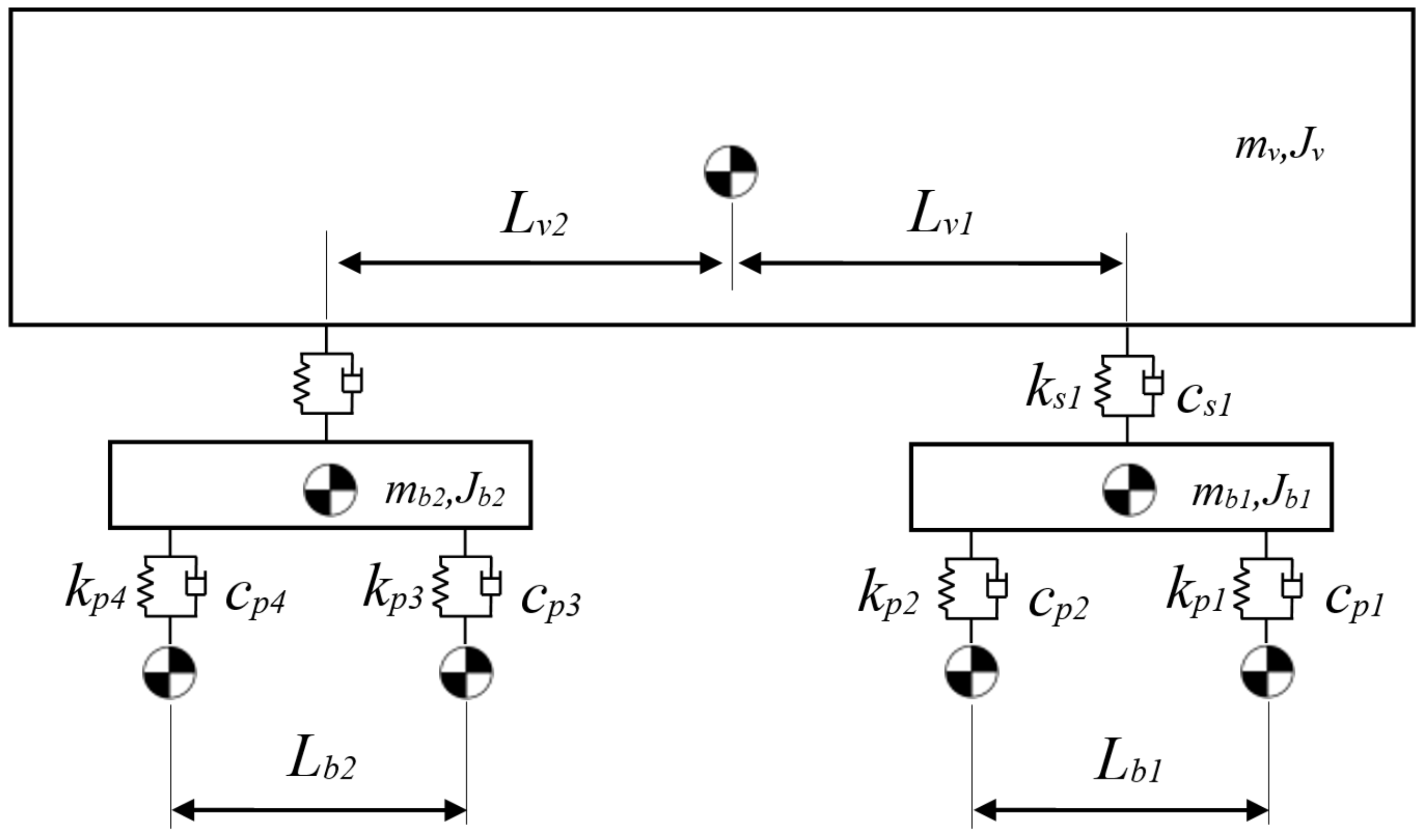
2.2. Train Model
2.3. Interaction
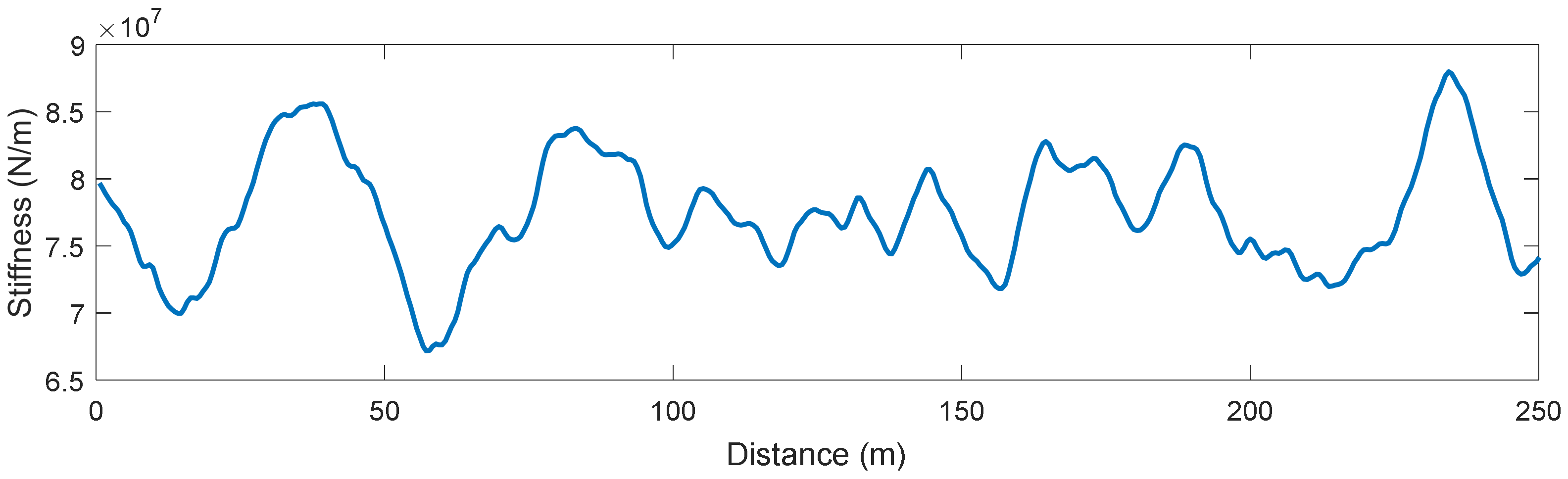
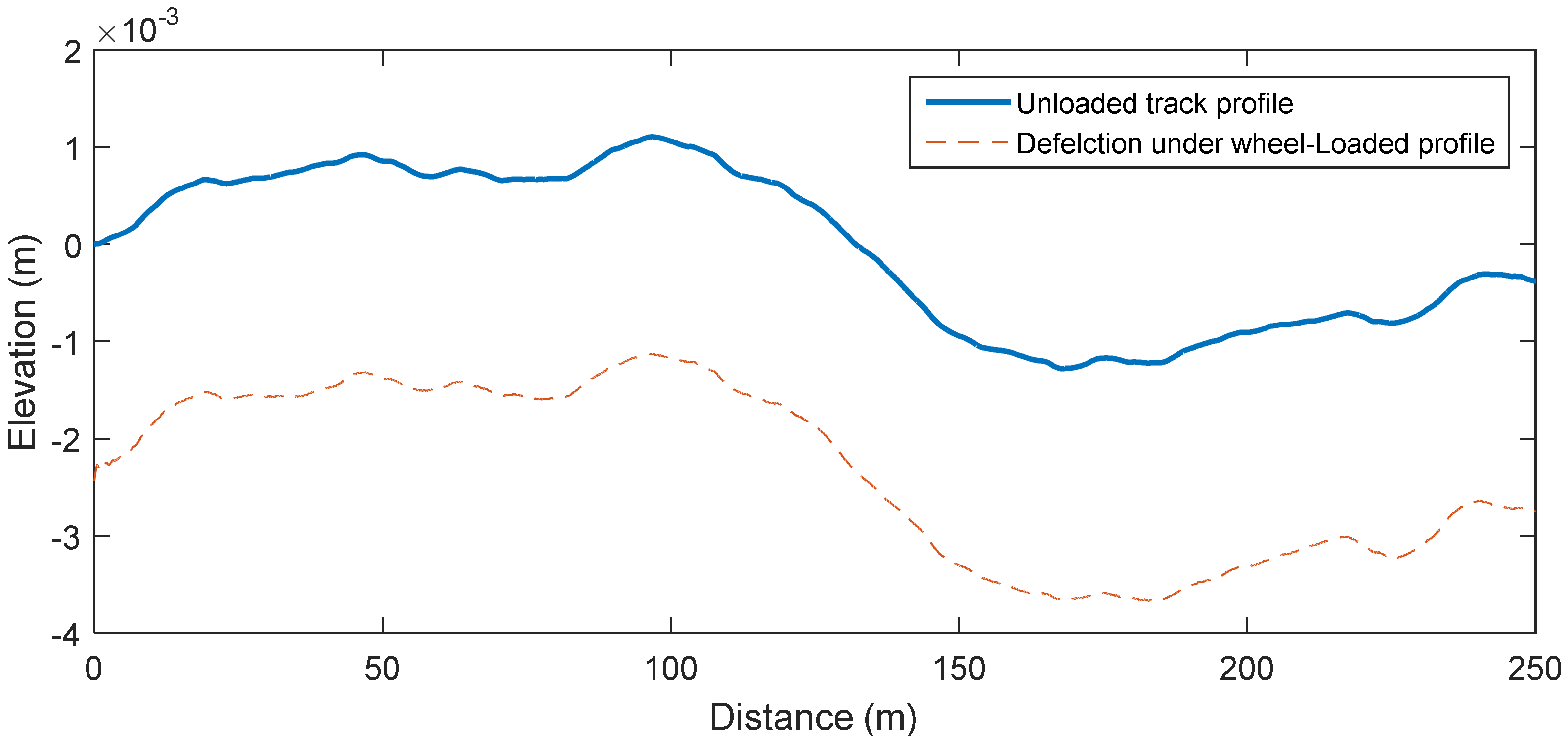
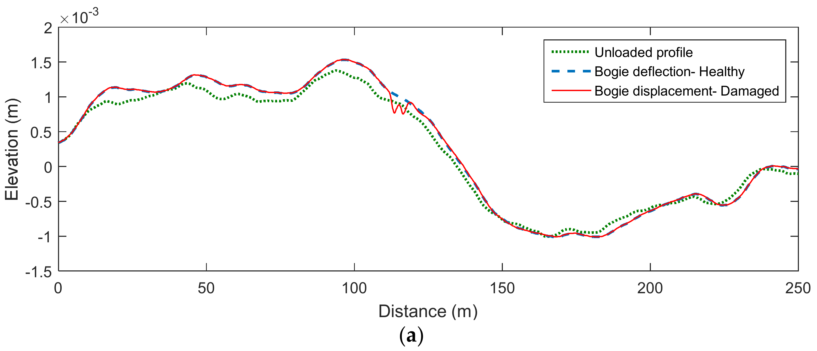
3. Track Longitudinal Profile and BFD
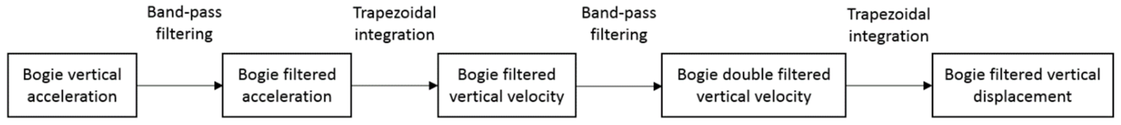
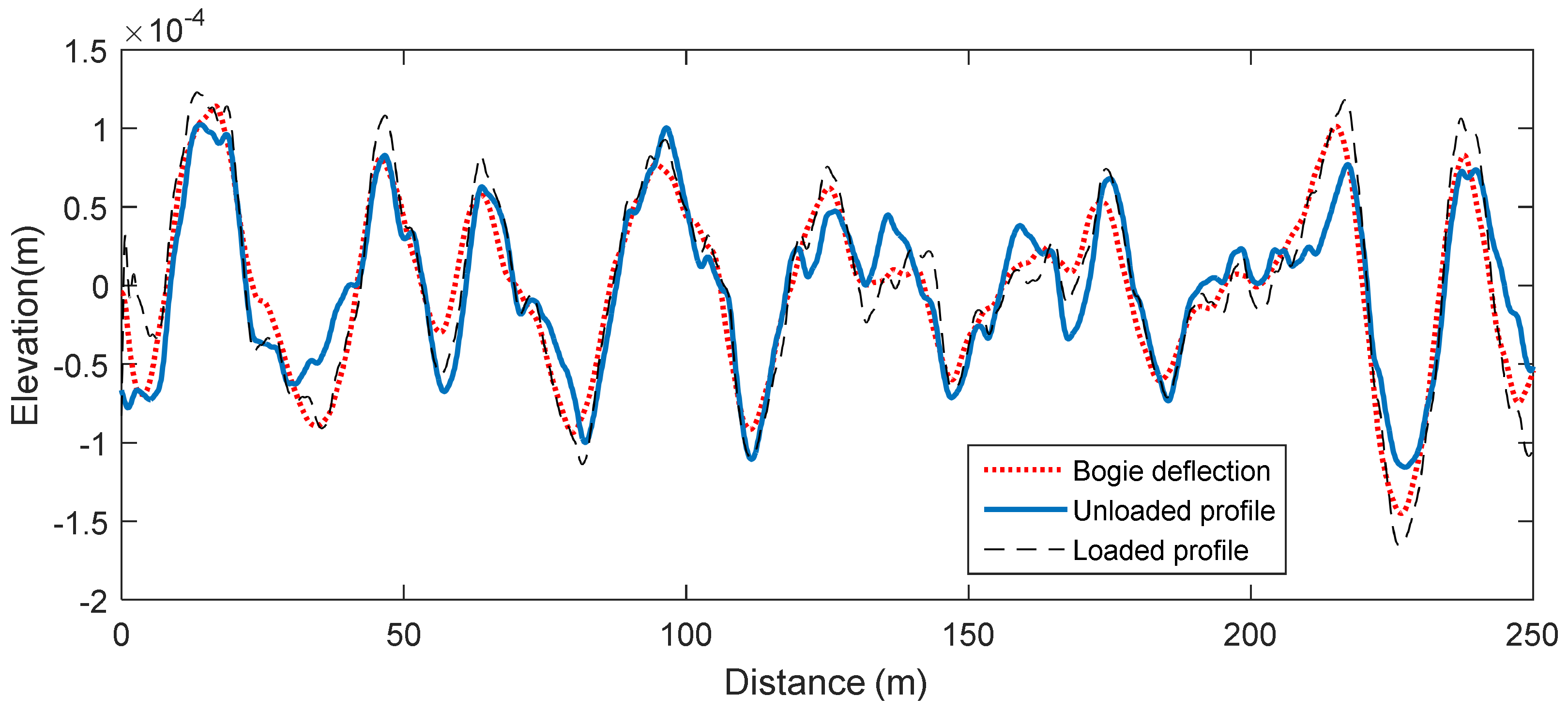
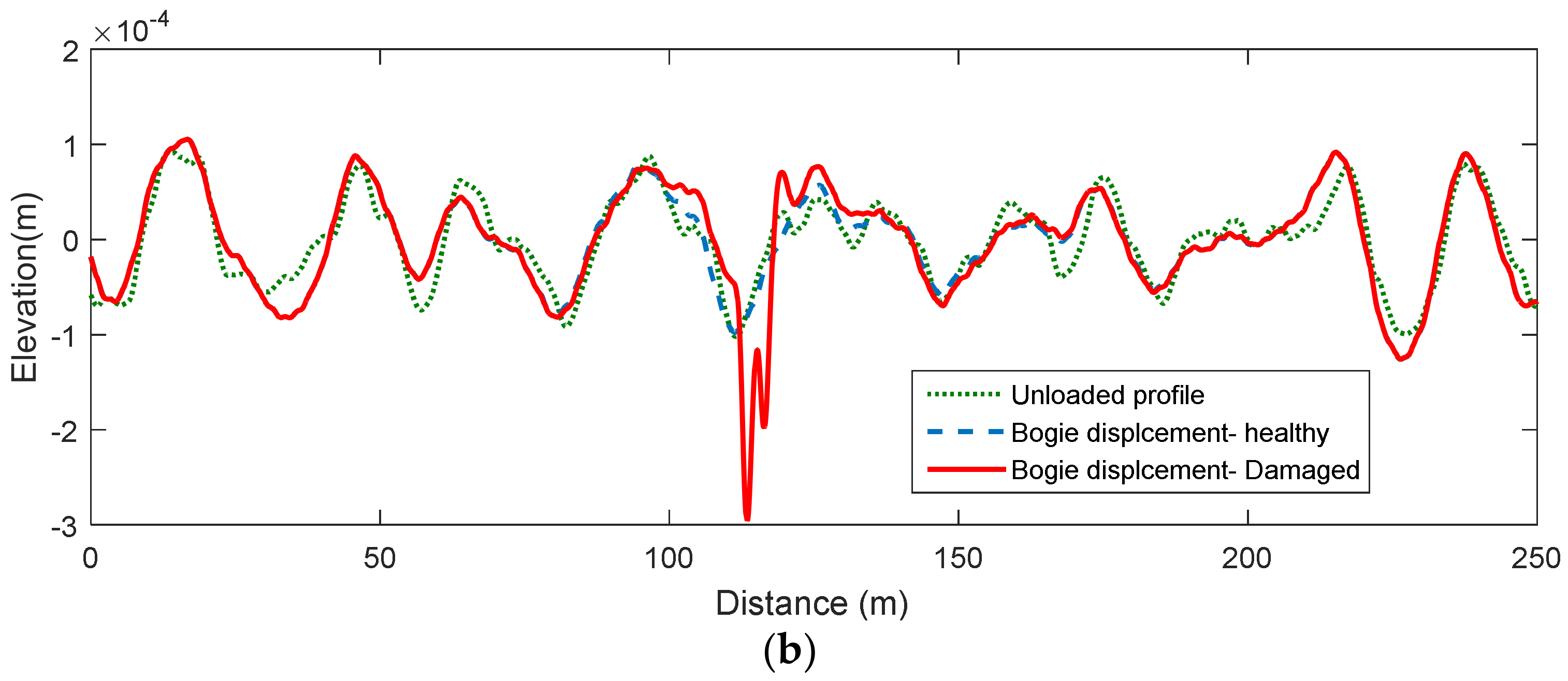
3.1. Bogie Filtered Displacement
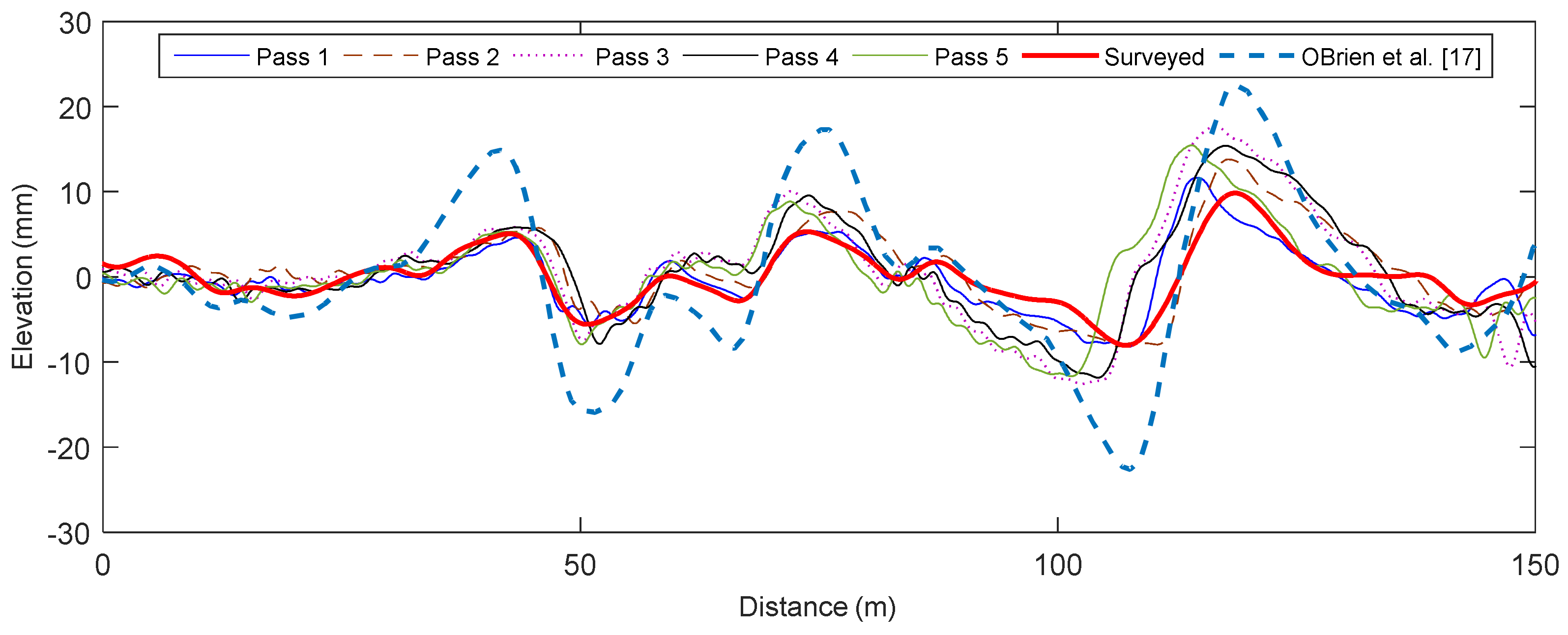
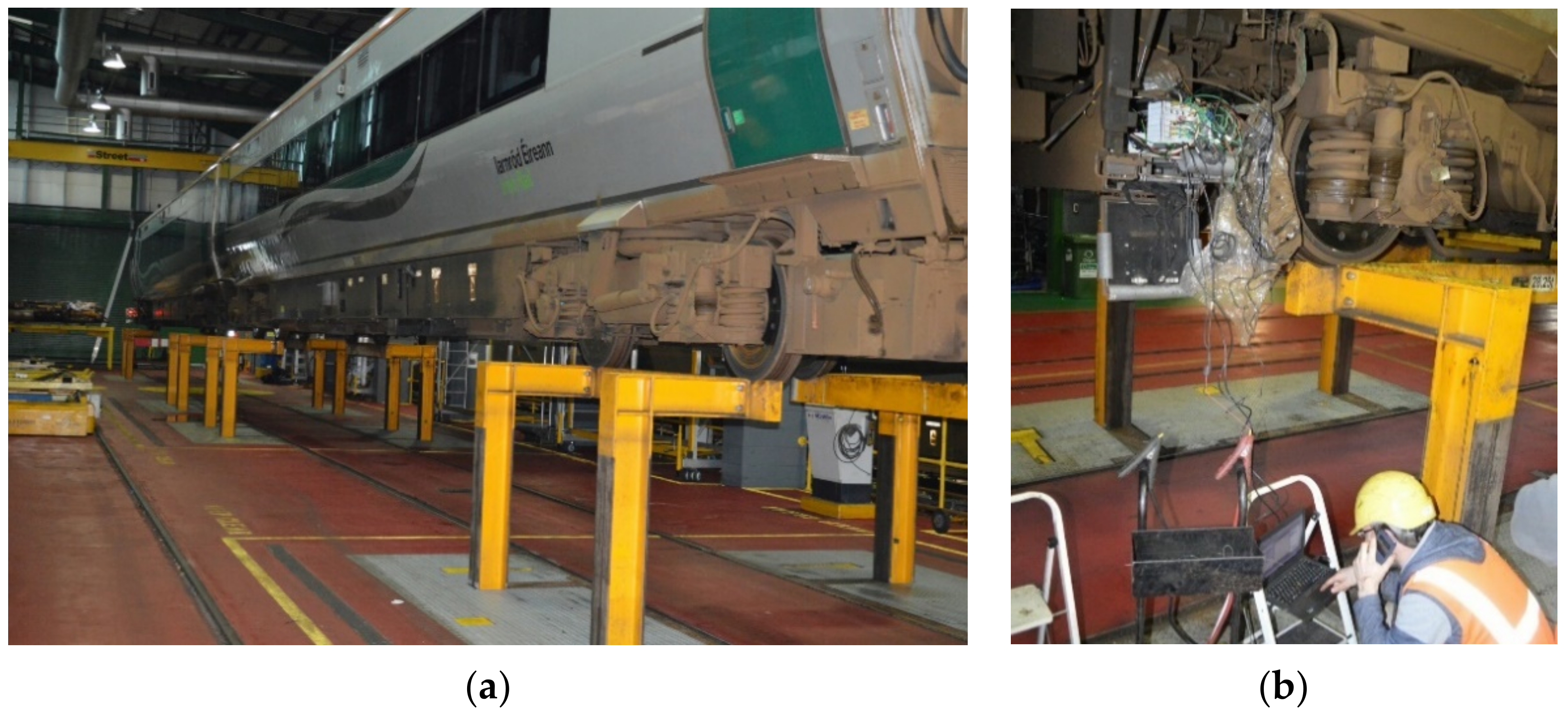
3.2. Experimental Verification
4. Track Condition Monitoring Using the BFD
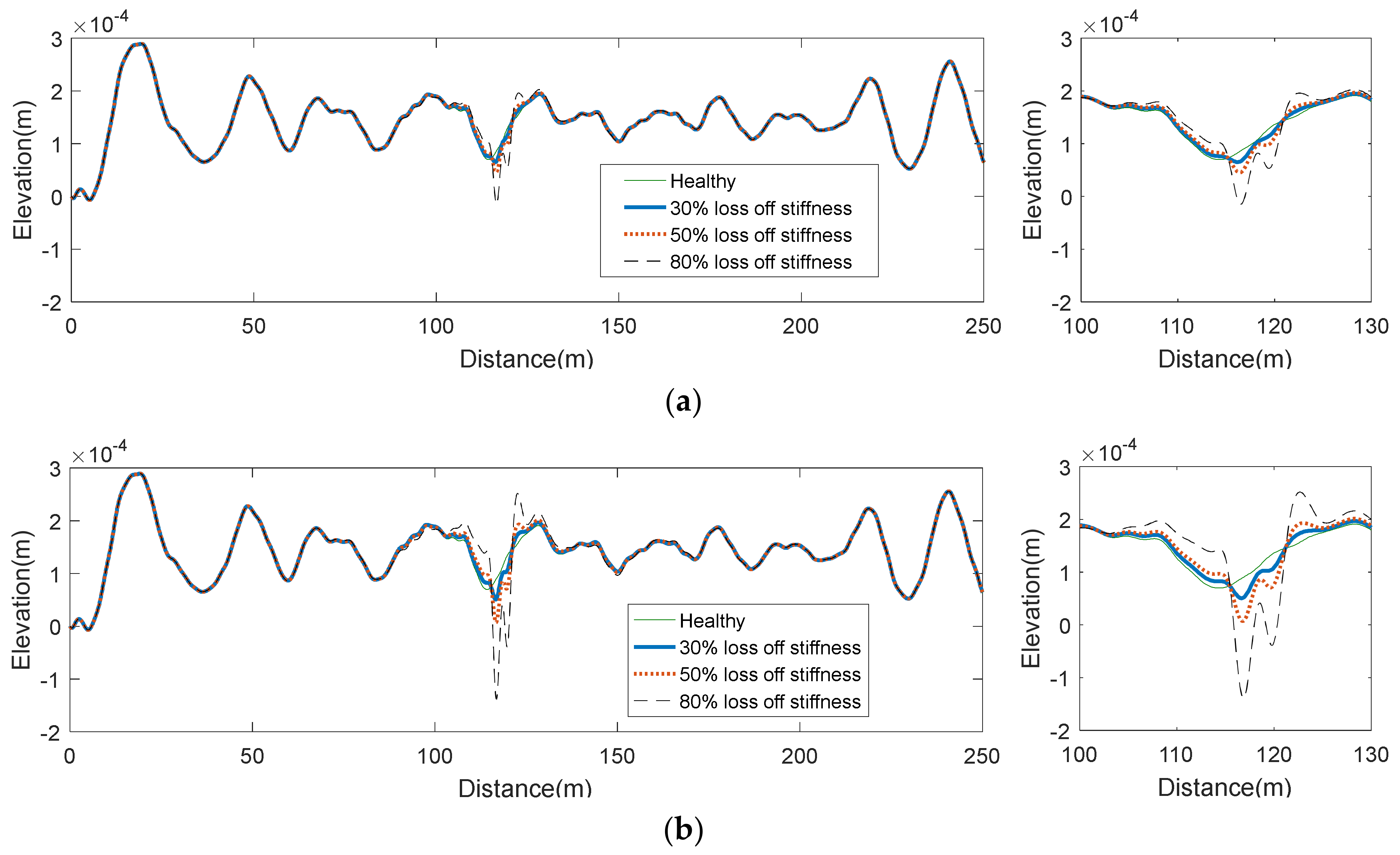
4.1. Loss of Stiffness at Subgrade Layer
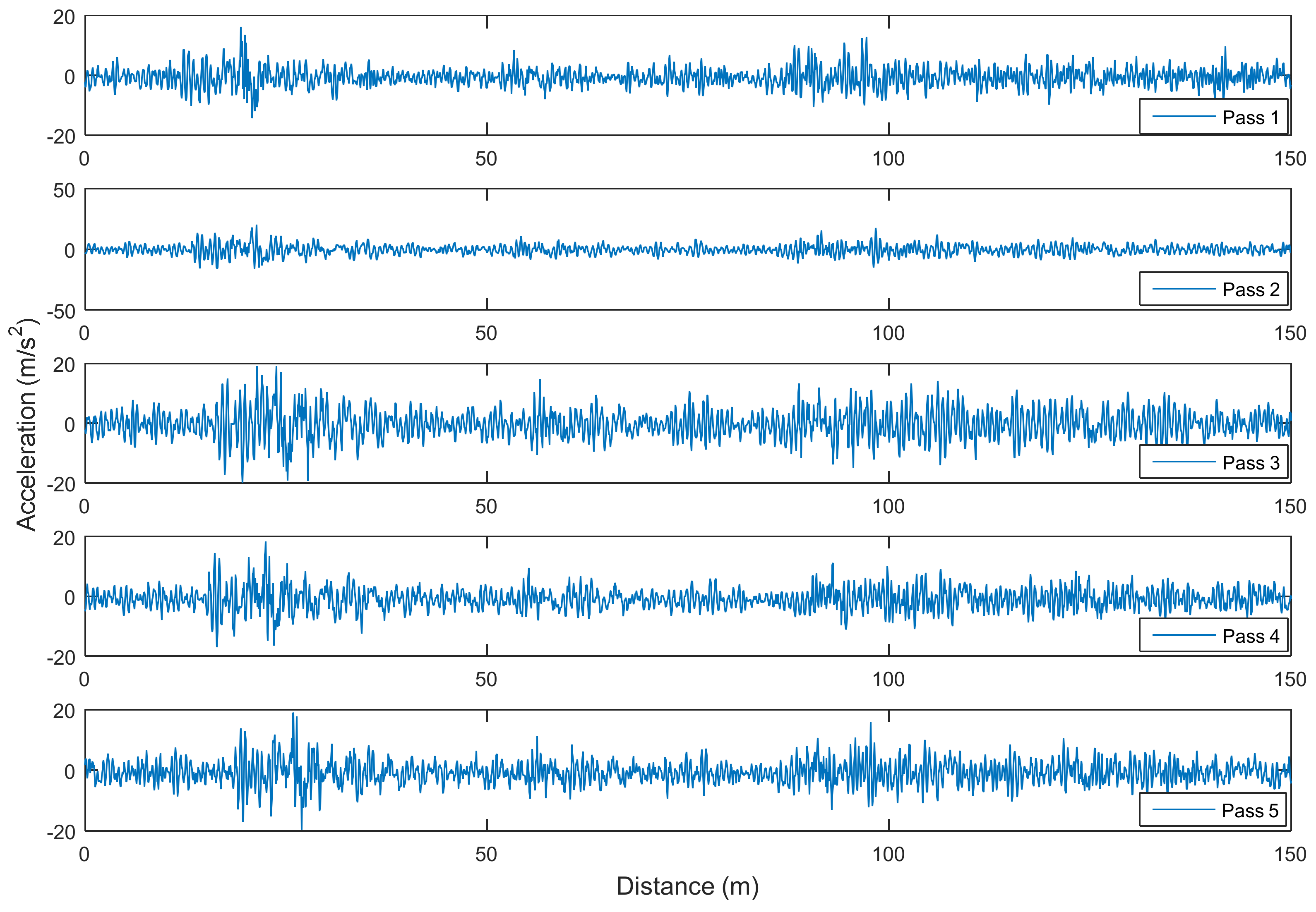
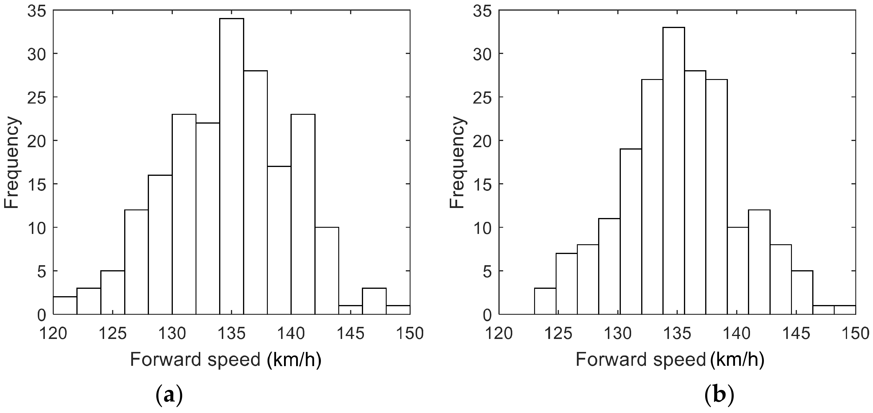
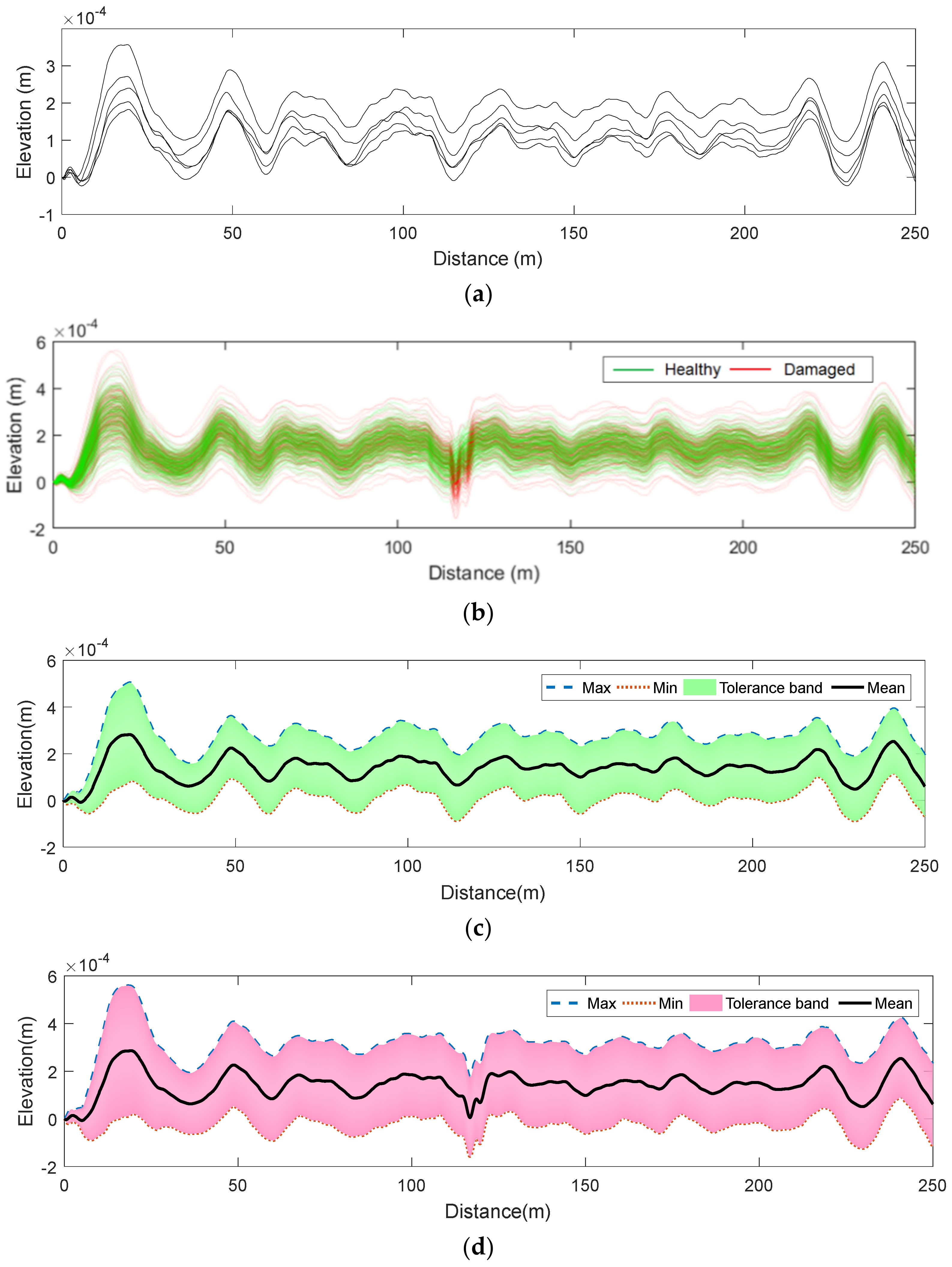
4.2. Multiple Runs in the Presence of Noise
5. Discussion
6. Conclusions
Author Contributions
Funding
Institutional Review Board Statement
Informed Consent Statement
Data Availability Statement
Conflicts of Interest
References
- Available online: https://erail.in/blog/countries-with-largest-railway-networks-in-world/50 (accessed on 21 June 2021).
- Gunn, D.A.; Chambers, J.E.; Dashwood, B.E.; Lacinska, A.; Dijkstra, T.; Uhlemann, S.; Swift, R.; Kirkham, M.; Milodowski, A.; Wragg, J.; et al. Deterioration model and condition monitoring of aged railway embankment using non-invasive geophysics. Constr. Build. Mater. 2018, 170, 668–678. [Google Scholar] [CrossRef] [Green Version]
- Kaewunruen, S.; Remennikov, A.M. Field trials for dynamic characteristics of railway track and its components using impact excitation technique. NDT E Int. 2007, 40, 510–519. [Google Scholar] [CrossRef]
- Malekjafarian, A.; OBrien, E.J.; Golpayegani, F. Indirect monitoring of critical transport infrastructure: Data analysis and signal processing. In Data Anlytics Applications for Smart Cities; Alavi, A.H., Buttlar, W.G., Eds.; Auerbach/CRC Press: Boca Raton, FL, USA, 2018. [Google Scholar]
- Berggren, E.G.; Nissen, A.; Paulsson, B.S. Track deflection and stiffness measurements from a track recording car. Proc. Inst. Mech. Eng. Part F J. Rail Rapid Transit 2014, 228, 570–580. [Google Scholar] [CrossRef]
- Wei, Z.L.; Nunez, A.; Li, Z.L.; Dollevoet, R. Evaluating Degradation at Railway Crossings Using Axle Box Acceleration Measurements. Sensors 2017, 17, 2236. [Google Scholar] [CrossRef] [Green Version]
- Barke, D.; Chiu, W.K. Structural health monitoring in the railway industry: A review. Struct. Health Monit. 2005, 4, 81–93. [Google Scholar] [CrossRef]
- Liu, C.; Wei, J.H.; Zhang, Z.X.; Liang, J.S.; Ren, T.Q.; Xu, H.Q. Design and evaluation of a remote measurement system for the online monitoring of rail vibration signals. Proc. Inst. Mech. Eng. Part F J. Rail Rapid Transit 2016, 230, 724–733. [Google Scholar] [CrossRef]
- Mennella, F.; Laudati, A.; Esposito, M.; Cusano, A.; Cutolo, A.; Giordano, M.; Campopiano, S.; Breglio, G. Railway monitoring and train tracking by fiber Bragg grating sensors. Proc. SPIE 2007, 6619. [Google Scholar] [CrossRef]
- Kerrouche, A.; Boyle, W.J.O.; Gebremichael, Y.; Sun, T.; Grattan, K.T.V.; Taljsten, B.; Bennitz, A. Field tests of fibre Bragg grating sensors incorporated into CFRP for railway bridge strengthening condition monitoring. Sens. Actuator A Phys. 2008, 148, 68–74. [Google Scholar] [CrossRef]
- Jönsson, J.; Arasteh Khouy, I.; Lundberg, J.; Rantatalo, M.; Nissen, A. Measurement of vertical geometry variations in railway turnouts exposed to different operating conditions. Proc. Inst. Mech. Eng. Part F J. Rail Rapid Transit 2016, 230, 486–501. [Google Scholar] [CrossRef]
- Sae Siew, J.; Mirza, O.; Kaewunruen, S. Torsional effect on track-support structures of railway turnouts crossing impact. J. Transp. Eng. Part A Syst. 2017, 143, 06016001. [Google Scholar] [CrossRef] [Green Version]
- Kampczyk, A. Measurement of the geometric center of a turnout for the safety of railway infrastructure using MMS and total station. Sensors 2020, 20, 4467. [Google Scholar] [CrossRef]
- Kaewunruen, S.; Dindar, S. The Effect of Climate Change on Service Life and Cost Investigation of Rail Turnouts with Various Mitigation Methods. In Inter-Noise and Noise-Con Congress and Conference Proceedings; Institute of Noise Control Engineering: Reston, VA, USA, 2018; pp. 6091–6101. [Google Scholar]
- Kampczyk, A. Railway Special Grid in Near Field Communication Technology for Rail Transport Infrastructure. In Transport Development Challenges in the 21st Century: Proceedings of the 2019 TranSopot Conference; Springer Nature: Berlin/Heidelberg, Germany, 2021; p. 87. [Google Scholar]
- Klug, F.; Lackner, S.; Lienhart, W. Monitoring of railway deformations using distributed fiber optic sensors. In Proceedings of the Joint International Symposium on Deformation Monitoring (JISDM), Vienna, Austria, 30 March–1 April 2016. [Google Scholar]
- Kampczyk, A. Magnetic-Measuring Square in the Measurement of the Circular Curve of Rail Transport Tracks. Sensors 2020, 20, 560. [Google Scholar] [CrossRef] [Green Version]
- Bocciolone, M.; Caprioli, A.; Cigada, A.; Collina, A. A measurement system for quick rail inspection and effective track maintenance strategy. Mech. Syst. Signal Process. 2007, 21, 1242–1254. [Google Scholar] [CrossRef]
- Molodova, M.; Li, Z.L.; Dollevoet, R. Axle box acceleration: Measurement and simulation for detection of short track defects. Wear 2011, 271, 349–356. [Google Scholar] [CrossRef]
- Lederman, G.; Chen, S.H.; Garrett, J.; Kovacevic, J.; Noh, H.Y.; Bielak, J. Track-monitoring from the dynamic response of an operational train. Mech. Syst. Signal Process. 2017, 87, 1–16. [Google Scholar] [CrossRef] [Green Version]
- Malekjafarian, A.; OBrien, E.J.; Cantero, D. Railway track monitoring using drive-by measurements. In Proceedings of the Fifteenth East Asia-Pacific Conference on Structural Engineering and Construction (EASEC-15), Xi’an, China, 11–13 October 2017. [Google Scholar]
- Fitzgerald, P.C.; Malekjafarian, A.; Cantero, D.; OBrien, E.J.; Prendergast, L.J. Drive-by scour monitoring of railway bridges using a wavelet-based approach. Eng. Struct. 2019, 191, 1–11. [Google Scholar] [CrossRef]
- Bowe, C.; Quirke, P.; Cantero, D.; O’Brien, E.J. Drive-by structural health monitoring of railway bridges using train mounted accelerometers. In Proceedings of the 5th ECCOMAS Thematic Conference on Computational Methods in Structural Dynamics and Earthquake Engineering, Crete Island, Greece, 25–27 May 2015. [Google Scholar]
- Nafari, S.F.; Gul, M.; Roghani, A.; Hendry, M.T.; Cheng, J.J.R. Evaluating the potential of a rolling deflection measurement system to estimate track modulus. Proc. Inst. Mech. Eng. Part F J. Rail Rapid Transit 2018, 232, 14–24. [Google Scholar] [CrossRef]
- Bar-Am, M. On-Train Rail Track Monitoring System. U.S. Patents US8942426B2, 27 January 2015. [Google Scholar]
- Fosburgh, B.A.; Nichols, M.E.; Holmgren, P.M.; Larsson, N.T. Railway Track Monitoring. US Patents US20120274772A1, 7 November 2017. [Google Scholar]
- OBrien, E.J.; Quirke, P.; Bowe, C.; Cantero, D. Determination of railway track longitudinal profile using measured inertial response of an in-service railway vehicle. Struct. Health Monit. 2017, 17, 1425–1440. [Google Scholar] [CrossRef]
- Zemp, A.; Muller, R.; Hafner, M. Characterization of Train-Track Interactions based on Axle Box Acceleration Measurements for Normal Track and Turnout Passages. In Proceedings of the 9th International Conference on Structural Dynamics (Eurodyn 2014), Porto, Portugal, 30 June–2 July 2014; pp. 827–833. [Google Scholar]
- Oregui, M.; Li, S.; Nunez, A.; Li, Z.; Carroll, R.; Dollevoet, R. Monitoring bolt tightness of rail joints using axle box acceleration measurements. Struct. Control Health Monit. 2017, 24, e1848. [Google Scholar] [CrossRef] [Green Version]
- Molodova, M.; Oregui, M.; Nunez, A.; Li, Z.L.; Dollevoet, R. Health condition monitoring of insulated joints based on axle box acceleration measurements. Eng. Struct. 2016, 123, 225–235. [Google Scholar] [CrossRef] [Green Version]
- Salvador, P.; Naranjo, V.; Insa, R.; Teixeira, P. Axlebox accelerations: Their acquisition and time-frequency characterisation for railway track monitoring purposes. Measurement 2016, 82, 301–312. [Google Scholar] [CrossRef] [Green Version]
- Cantero, D.; Basu, B. Railway infrastructure damage detection using wavelet transformed acceleration response of traversing vehicle. Struct. Control Health Monit. 2015, 22, 62–70. [Google Scholar] [CrossRef]
- Quirke, P.; Cantero, D.; OBrien, E.J.; Bowe, C. Drive-by detection of railway track stiffness variation using in-service vehicles. Proc. Inst. Mech. Eng. Part F J. Rail Rapid Transit 2017, 231, 498–514. [Google Scholar] [CrossRef] [Green Version]
- Brien, E.J.O.; Bowe, C.; Quirke, P.; Cantero, D. Determination of longitudinal profile of railway track using vehicle-based inertial readings. Proc. Inst. Mech. Eng. Part F J. Rail Rapid Transit 2017, 231, 518–534. [Google Scholar] [CrossRef] [Green Version]
- Odashima, M.; Azami, S.; Naganuma, Y.; Mori, H.; Tsunashima, H. Track geometry estimation of a conventional railway from car-body acceleration measurement. Mech. Eng. J. 2017, 4. [Google Scholar] [CrossRef] [Green Version]
- Malekjafarian, A.; OBrien, E.; Quirke, P.; Bowe, C. Railway Track Monitoring Using Train Measurements: An Experimental Case Study. Appl. Sci. 2019, 9, 4859. [Google Scholar] [CrossRef] [Green Version]
- Cantero, D.; Arvidsson, T.; OBrien, E.; Karoumi, R. Train-track-bridge modelling and review of parameters. Struct. Infrastruct. Eng. 2016, 12, 1051–1064. [Google Scholar] [CrossRef]
- Zhai, W.M.; Wang, K.Y.; Cai, C.B. Fundamentals of vehicle-track coupled dynamics. Veh. Syst. Dyn. 2009, 47, 1349–1376. [Google Scholar] [CrossRef]
- Lu, F.; Kenned, D.; William, F.W.; Lin, J.H. Symplectic analysis of vertical random vibration for coupled vehicle-track systems. J. Sound Vib. 2008, 317, 236–249. [Google Scholar] [CrossRef]
- Nguyen, K.; Goicolea, J.M.; Galbadon, F. Comparison of dynamic effects of high-speed traffic load on ballasted track using a simplified two-dimensional and full three-dimensional model. Proc. Inst. Mech. Eng. Part F J. Rail Rapid Transit 2014, 228, 128–142. [Google Scholar] [CrossRef]
- Zhai, W.M.; Wang, K.Y.; Lin, J.H. Modelling and experiment of railway ballast vibrations. J. Sound Vib. 2004, 270, 673–683. [Google Scholar] [CrossRef]
- Lei, X.; Noda, N.A. Analyses of dynamic response of vehicle and track coupling system with random irregularity of track vertical profile. J. Sound Vib. 2002, 258, 147–165. [Google Scholar] [CrossRef]
- Sun, Y.Q.; Dhanasekar, M. A dynamic model for the vertical interaction of the rail track and wagon system. Int. J. Solids Struct. 2002, 39, 1337–1359. [Google Scholar] [CrossRef]
- Lou, P. Finite element analysis for train-track-bridge interaction system. Arch. Appl. Mech. 2007, 77, 707–728. [Google Scholar] [CrossRef]
- Goicolea Ruigómez, J.M. Unofficial Description of Loads and Masses of High Speed Train in Spanish Network AVE S-103 (Siemens ICE3 Velaro); E.T.S.I. Caminos, Canales y Puertos (UPM): Madrid, Spain, 2014. [Google Scholar]
- Kaynia, A.M.; Park, J.; Noren-Cosgriff, K. Effect of track defects on vibration from high speed train. In Proceedings of the International Conference on Structural Dynamics (Eurodyn 2017), Rome, Italy, 10–13 September 2017; pp. 2681–2686. [Google Scholar]


| Property | Unit | Value |
|---|---|---|
| Elastic modulus of rail | N/m2 | 2.059 × 10¹¹ |
| Rail cross-sectional area | m2 | 7.69 × 10⁻³ |
| Rail second moment of area | m4 | 3.217 × 10⁻⁵ |
| Rail mass per unit length | kg/m | 60.64 |
| Rail pad stiffness | N/m | 6.5 × 10⁷ |
| Rail pad damping | Ns/m | 7.5 × 10⁴ |
| Sleeper mass (half) | kg | 125.5 |
| Sleeper spacing | m | 0.545 |
| Ballast stiffness | N/m | 137.75 × 10⁶ |
| Ballast damping | Ns/m | 5.88 × 10⁴ |
| Ballast mass | kg | 531.4 |
| Subgrade stiffness mean | N/m | 77.5 × 10⁶ |
| Subgrade damping | Ns/m | 3.115 × 10⁴ |
| Property | Symbol | Unit | Value |
|---|---|---|---|
| Wheelset mass | mw | kg | 1800 |
| Bogie mass | mb | kg | 3500 |
| Car body mass | mv | kg | 47,800 |
| Moment of inertia of bogie | Jb | kg.m2 | 1715 |
| Moment of inertia of main body | Jv | kg.m2 | 1.96 × 10⁶ |
| Primary suspension stiffness | kp | N/m | 2.4 × 10⁶ |
| Secondary suspension stiffness | ks | N/m | 0.7 × 10⁶ |
| Primary suspension damping | cp | Ns/m | 20 × 103 |
| Secondary suspension damping | cs | Ns/m | 40 × 103 |
| Distance between car body center of mass and bogie pivot | Lv1, Lv2 | m | 8.6875 |
| Distance between axles | Lb1, Lb2 | m | 2.5 |
| Sensor Location | Type | Name | Range |
|---|---|---|---|
| Bogie–Bounce | Triaxial Accelerometer | Disynet-DA3802-015g | ±15 g |
| Bogie–Pitch | Triaxial Gyrometer | Crossbow VG400CC-200 | ±200°/s |
Publisher’s Note: MDPI stays neutral with regard to jurisdictional claims in published maps and institutional affiliations. |
© 2021 by the authors. Licensee MDPI, Basel, Switzerland. This article is an open access article distributed under the terms and conditions of the Creative Commons Attribution (CC BY) license (https://creativecommons.org/licenses/by/4.0/).
Share and Cite
Malekjafarian, A.; OBrien, E.J.; Quirke, P.; Cantero, D.; Golpayegani, F. Railway Track Loss-of-Stiffness Detection Using Bogie Filtered Displacement Data Measured on a Passing Train. Infrastructures 2021, 6, 93. https://0-doi-org.brum.beds.ac.uk/10.3390/infrastructures6060093
Malekjafarian A, OBrien EJ, Quirke P, Cantero D, Golpayegani F. Railway Track Loss-of-Stiffness Detection Using Bogie Filtered Displacement Data Measured on a Passing Train. Infrastructures. 2021; 6(6):93. https://0-doi-org.brum.beds.ac.uk/10.3390/infrastructures6060093
Chicago/Turabian StyleMalekjafarian, Abdollah, Eugene J. OBrien, Paraic Quirke, Daniel Cantero, and Fatemeh Golpayegani. 2021. "Railway Track Loss-of-Stiffness Detection Using Bogie Filtered Displacement Data Measured on a Passing Train" Infrastructures 6, no. 6: 93. https://0-doi-org.brum.beds.ac.uk/10.3390/infrastructures6060093