Article

Are the Purchase Prices of Solar Energy Projects under Development Consistent with Cost of Capital Forecasts?

by
Miguel Vázquez-Vázquez
,
Ana B. Alonso-Conde
* and
Javier Rojo-Suárez
Department of Business Administration, Rey Juan Carlos University, Paseo de los Artilleros s/n, 28032 Madrid, Spain
*
Author to whom correspondence should be addressed.
Submission received: 28 May 2021 / Revised: 18 June 2021 / Accepted: 20 June 2021 / Published: 22 June 2021
(This article belongs to the Section Sustainable Infrastructures)

Abstract

:
The reduction in construction and maintenance costs per MW of renewable energy facilities, together with low interest rates, have led to a significant growth in the purchase prices paid for these facilities in the Spanish market. This trend is shared by other European countries, especially for projects that hedge energy price risk incorporating power purchase agreements with third parties. In this framework, questions arise about the economic rationale of the purchase prices paid for these projects. Consequently, we develop a project evaluation model that forecasts expected cash flow and time-varying required rates of return for a standard photovoltaic plant, in order to study the extent to which foreseeable market conditions—interest rates and equity risk premia, among others—translate into economically viable buyouts. Our results suggest that purchase prices paid for these initiatives often lead to buyer returns below those that would be reasonable according to market conditions. Indeed, we find that only facilities that reach a production 23% higher than the number of hours considered in the base case provide returns that compensate long-term financing costs. However, specialised investors can exploit their relatively low cost of financing to pay prices up to 73% higher than those affordable by classic investors.

Graphical Abstract

1. Introduction

Renewable energy has become a key priority in many geographical areas as it provides clean and sustainable energy, among other benefits, to companies and households [1,2,3,4]. Furthermore, investment in renewable energy is crucial to achieving the ambitious climate targets outlined in the Paris Agreement, where large investments in infrastructure are required to ensure growth and meet the basic needs of the population in developed countries [5]. Hence, according to OECD estimates [6], economic growth requires an investment in infrastructure (energy, transport, water or telecommunications) of around 95 trillion dollars from 2016 to 2030, that is, 6.3 trillion dollars per year, ignoring purely climate considerations. Moreover, for the infrastructure supply to be consistent with the 2 °C global temperature target, investments of 6.9 trillion dollars per year are required, although climate variability would persist [7]. All these elements make it essential to properly organise and structure the financing circuit for the energy transition [8].
In this framework, recent trends in renewables depict a scenario that involves a race for licenses and locations, where investors are willing to pay relatively high prices for projects that are not under construction and, in some cases, not even ready-to-build (RTB) [9]. Low interest rates and cost reduction largely determine this fact. In the specific case of the Spanish market, photovoltaic projects have experienced strong reductions in capital expenditures (CapEx) and operational expenses (OpEx), with CapEx falling on average from 6.000 € k/MW to around 500–600 € k/MW, and OpEx falling from 50 €/MWh to 20–25 €/MWh. This environment has allowed installed capacity to exceed 50,000 MW in 2019, with wind projects exceeding 25,000 MW and solar plants 11,000 MW [10].
As a result, the Spanish renewable energy industry is attracting significant attention from a wide range of investors willing to undertake new renewable energy projects. In fact, in 2019, the sole transmission agent and operator of the national electricity system in Spain—Red Eléctrica de España—received requests amounting to 125,200 MW, which is well above the expected capacity for Spain until 2030, according to the forecasts of the Spanish Government (48,550 MW of installed capacity for wind projects and 38,404 MW for photovoltaic plants, according to the National Energy and Climate Plan 2021–2030). This environment has led to an increase in purchase prices paid for RTB facilities—reaching 100–200 €/MW according to data from Mergermarket database—with large utilities, energy providers and financial investors acting generally as buyers. This framework raises the question of the economic rationale behind the prices paid for RTB projects.
Accordingly, based on the growing interest in promoting renewable energy within the framework of the climate targets of the European Union, as well as the results of previous literature that emphasises the existence of a green bubble [11,12,13], in this paper we compare the internal rate of return (IRR) of a standard photovoltaic plant located in Spain, with the cost of equity required by different types of investors who usually channel funds to these projects, in particular, domestic utility companies and foreign solar funds. Hence, using an approach similar to that followed by Martín et al. [14], we study the existence of economic reasons that explain the purchase prices of photovoltaic projects. Specifically, building on the fact that renewable energy projects should guarantee a net present value (NPV) equal to or greater than zero to ensure their economic viability, we study whether this is often the case under current market conditions or whether inflated purchase prices consistently translate into negative NPV. Importantly, Martín, Coronas, Alonso, de la Hoz and Matas [14] find that the onshore wind and photovoltaic auctions in Denmark in 2019 require very specific scenarios to be viable, raising doubts about their effective implementation. For example, in the specific case of photovoltaic energy in the Danish market, the authors show that this energy source is not profitable for any WACC, concluding that either a 60% discount on the investment cost or an annual increase of 6.8% in the market price is required for the NPV to reach the breakeven point.
From a methodological perspective, our approach combines classic methods commonly used to evaluate investments—i.e., the IRR and the NPV—with other models provided by the asset pricing theory—e.g., the Vasicek [15] model or the Campbell and Shiller [16] model—that allow us to account for the time-varying nature of discount rates. Importantly, although constant discount rates are frequently used in practice to evaluate new investment projects, abnormally high or low market returns can lead to underestimating or overestimating project performance, thereby hindering well-informed investment decisions. Furthermore, time-varying discount rates are central to correctly evaluating finite-life projects, given their lower indebtedness over time. Therefore, this paper contributes to filling de gap between the classic project evaluation techniques and the recent findings provided by the asset pricing theory. Moreover, we use our model to study the average number of operation hours that allows the project to provide an IRR that covers the implied cost of equity throughout the project life, as well as the maximum purchase price affordable for a notional utility company located in Spain and a generic infrastructure fund located in UK, under current market conditions. In this regard, it should be noted that most of the infrastructure funds operating in the renewable energy industry in Spain are located outside of this country and many of them are based in London. Consequently, for the sake of simplicity, we use a generic UK investor to represent this investor typology.
Our paper contributes to the previous literature in the following terms. First, to the best of our knowledge, this is the first study to analyse the rationale behind the purchase price of RTB solar plants in Spain, using conditional discount rates to capture the effect of the current level of interest rates and equity risk premia in the performance of the project. Second, our results provide updated projections in the performance of Spanish photovoltaic plants. These projections are fully consistent with the current regulatory framework in this country, thus expanding our knowledge of current trends in renewables. Third, our model helps reconcile some widely recognised asset pricing models in the literature with classic procedures used in practice to determine discount rates, allowing us to realistically estimate the conditional cost of equity of photovoltaic projects. In particular, our approach allows us to determine time-varying discount rates that are fully consistent with the current conditions of financing markets. Furthermore, our model helps us control the NPV of the project for the current level of both the risk-free rate and equity risk premium, which allows us to avoid that our results artificially reject the market overvaluation, especially given the low level of interest rates at the valuation date. Finally, our methodology helps us to capture the effects of the purchase power of some international investors on project prices, given their relatively low cost of capital.
The remainder of the paper is organised as follows. Section 2 describes the model. Section 3 presents and discusses the empirical results. Finally, Section 4 concludes the paper.

2. Materials and Methods

2.1. Operational and Financial Assumptions

In this subsection we describe the operational and financial assumptions established to evaluate the apparent overvaluation of the purchase prices paid for solar facilities in Spain at the beginning of 2020. For that purpose, we study a generic photovoltaic project that has not yet started construction, using information consistent with data from different operations in the Spanish renewable energy market at the valuation date. The main operational assumptions are summarised in Table 1.
At this point, it should be noted that the current regulatory framework for renewable energies in Spain highlights different sources of uncertainty, such as the volatility in the price of energy or pool price. This fact has greatly encouraged the use of power purchase agreements (PPAs) to hedge buyers against energy price volatility both in wind and solar projects [17,18], where PPA contractual terms are often protected by nondisclosure agreements, and publicly available corporate data is usually of limited utility. In this context, our base case assumes a nominal installed capacity of 40 MW, with an operating life of 30 years. Based on data from recent photovoltaic projects, we assume a production level of 2200 net hours per year, with 90% of the production sold through a PPA contract and the remaining production sold at the pool price. Figure 1 shows the price curve and PPA prices that result from our assumptions.
We use data provided by independent experts to configure the price curve projections shown in Figure 1, assuming a capture rate of 100.36%, consistent with Spanish regulation (Orden TED/17/2000). Regarding PPA prices, interestingly, Miller et al. [19] and Mendicino, Menniti, Pinnarelli and Sorrentino [17] analyse their relationship with the levelised cost of energy (LCOE) for estimation purposes. However, for the sake of simplicity, we use data from BloombergNEF [20] to set the PPA price to 35.30 €/MWh in January 2020. It should be noted that this price is consistent with the capacity, the term and the contractual structure of the project under study. Additionally, prices in Figure 1 assume an annual price increase of 1.5% to reflect inflation in the projections, according to CPI long term estimations for the Spanish Economy provided by the EIU Global Forecasting Service at the valuation date.
Regarding operational costs, heterogeneity in disclosure levels across companies and sources of data translates into significant barriers to establishing a standard base for comparison. Hence, Tegen et al. [21] report an average annual operational cost of 11 $/MWh for the US market, while Giberson [22] reports an annual operational cost for wind projects of 21 $/MWh. Consistent with the strong cost reduction experienced by renewable projects in Spain since 2016, we set operational expenses to 8.25 €/MWh or, equivalently, 13.25 € k/MW. Regarding CapEx, it should be mentioned that investment costs have experienced a sharp decrease in the last decade, with the prices of solar modules declining from 3.000–3.500 € k/MW in 2010 to less than 500 € k/MW in 2019 [23]. Using these data and including other supplementary costs (inverters, grid connection, cabling wiring, mechanical and electrical installation), we assume that CapEx in construction amounts to 580 €/MW in the base case, while it increases to 816 €/MW in the worst-case scenario, that is, a price increase of 40%, according to the volatility of the construction costs of solar projects in Spain in recent years.
Table 2 summarises the main financial assumptions established in our model. Remarkably, although bond financing, and in particular green bonds, is gaining increasing importance in funding sustainable projects [24,25,26], traditional project finance structures remain the most widely used financing instrument for individual energy projects. Accordingly, based on data from previous operations, we assume a debt-to-equity ratio of 70/30, where the principal is reimbursed according to a debt service coverage ratio (DSCR) of 1.25, and interest rate amounts to 2.50%, increasing 25 basis points every 5 years.
As noted in the following section, we determine discount rates using return data for different types of investors who typically channel funds to renewable energy projects. However, while those companies usually invest in turnkey facilities, the project under study is in the RTB stage, thus assuming construction risk. Importantly, the allocation of construction risk is key issue for infrastructure projects. Thus, Vassallo et al. [27] highlight the fact that pension funds, unlike commercial banks, are unwilling to bear construction risks given their lack expertise to properly assess them. On the other hand, quantitative procedures, such as stochastic simulation methods and computational intelligence techniques, are useful tools for analysing the uncertainty surrounding forecasts [28,29]. In this regard, for the purpose of our study, we assume that the sponsor bears all the construction risk, which translates into a higher cost of equity. To determine the expected increase in the cost of equity that results from construction risk, we use the scenarios shown in Table 1—i.e., the base case and the worst-case scenario—to run a Monte Carlo simulation that accounts for the main construction risks, namely: (i) the potential increase in construction costs, and (ii) the potential delay in the construction period. For that purpose, the worst-case scenario assumes that CapEx increases by 40% with respect to base case, while the construction delay comprises 6 months. Assuming that both CapEx and the construction period are uniformly distributed, the difference between the IRR for shareholders in the base case and the average IRR for shareholders provided by the Monte Carlo simulation results in a construction risk premium of 2.06%. Below we use this result to correct the estimated cost of equity for construction risk.

2.2. Discount Rates

Discount rates constitute a key element for most investment valuation models, as they represent the minimum expected rate of return required for the project throughout its operating life. From a practical perspective, the capital asset pricing model (CAPM) [30,31,32] is by far the most widely used model for determining discount rates, satisfying:
E ( R t + 1 i ) = k e i = R f + [ E ( R t + 1 m ) R f ] β i
where E ( R t + 1 i ) is the unconditional expected return for asset i, k e i is the unconditional cost of equity, R f is the risk-free rate, E ( R t + 1 m ) is the expected return of the wealth portfolio—usually proxied by a broad-based market portfolio—and β i is the slope coefficient that results from the regression of R t + 1 i on R t + 1 m . Accordingly, Expression (1) implicitly assumes that the wealth portfolio perfectly captures investor preferences and that expected returns are linearly related to betas.
However, despite its practical success, the CAPM has traditionally performed poorly in empirical research, providing beta coefficients weakly related to expected returns and near-zero cross-sectional R 2 statistics [33,34,35,36]. The fact that the portfolios used as a proxy for the wealth portfolio are often far from being mean-variance efficient and, especially, the forecastable nature of expected returns cause significant differences to emerge between the conditional and unconditional versions of the model [37,38,39,40]. Accordingly, the time-varying nature of the risk-free rate, the equity risk premium and beta coefficients largely explains the poor performance of the CAPM in practice.
Given the aforementioned limitations and the fact that Table 1 and Table 2 comprise early 2020 market data, we estimate the conditional cost of equity on an annual basis using the conditional version of Expression (1), which allows us to account for the time-varying nature of the CAPM components, as follows:
E ( R t + j i ) = k e , t + j i = R t + j f + [ E t ( R t + j m ) R t + j f ] β t + j i
where E t ( R t + j i ) is the expected return for asset i for the period from t + j − 1 to t + j conditional on time-t information, k e , t + j i is the conditional cost of equity, R t + j f is the risk-free rate from t + j − 1 to t + j, E t ( R t + j m ) is the expected return of the market portfolio conditional on time-t information, and β t + j i is the conditional beta coefficient.
To estimate future risk-free rates, we exploit the accuracy and tractability of the Vasicek [15] model to forecast the one-year Treasury Bill rate throughout the life of the project. Accordingly:
d R t f = a ( b R t f ) d t + σ d M t
where a is the speed of reversion of the current interest rate to its long-term mean level, b is long-term mean interest rate, σ is the instantaneous volatility, and W t is a Weiner process. Therefore, below we use the Euler approximation of Expression (3) to determine the expected pattern of the risk-free rate throughout the project file.
We determine the term structure of expected equity market returns E t ( R t + j m ) using the Campbell-Shiller present value decomposition, which allows us to consistently estimate the equity risk premium over time. Specifically, following Campbell and Shiller [16] and using lowercase letters to denote logs:
d p t j = 1 ρ j 1 r t + j j = 1 ρ j 1 Δ d t + j
where d p t is the dividend yield in logs at time t, r t + j is the log return, Δ d t + j is log dividend growth, and ρ = 1 / ( 1 + D P ) . The terms on the right-hand side of Expression (4) can be written as a function of the dividend yield, as follows:
j = 1 ρ j 1 r t + j = b r d p t + ε r
j = 1 ρ j 1 d t = b d d p t + ε d
where b r and b d are regression coefficients, and ε r and ε d are error terms. In the next section, we use Expression (5) in levels instead of logs, together with the AR(1) process of the dividend yield, to determine the expected pattern of the market return E t ( R t + j m ) , thus exploiting the persistent nature of the dividend yield over time, as well as its strong predictive power. This allows us to explicitly consider the term structure of expected returns—and consequently the predictability pattern of stock returns—in our analysis.
Regarding betas, unlike companies operating on an ongoing basis, project finance investments are characterised by indebtedness that decreases sharply over time. Since this fact can give rise to important effects on levered betas, we account for their time-varying nature using the Hamada [41] model, which satisfies:
β L , t = β U , t [ 1 + L t · ( 1 T t ) E t ]
where β L , t and β U , t are levered and unlevered betas, respectively, L t is the value of debt, E t is the equity value, and T t is the tax rate.
As shown in the following section, all the previous models allow us to reliably estimate the annual cost of equity for the investment under analysis and, consequently, the implied cost of equity throughout the life of the project.

3. Results and Discussion

In this section, we study the consistency between the expected IRR for shareholders of the photovoltaic project under analysis, according to assumptions in Table 1 and Table 2, and the cost of equity that results from the methodology described in the previous section. To analyse the extent to which the specific nature of the investor can result in significant variations in discount rates, we determine the cost of equity from two different perspectives. First, we use an equal-weighed portfolio comprising Spanish utility companies to estimate the cost of equity from the perspective of a Spanish notional investor. Second, using an analogous approach, we use an equal-weighed portfolio comprising shares issued by UK solar funds to estimate the cost of equity from the perspective of a UK notional investor.
On this basis, we use the assumptions in Table 1 and Table 2 to perform the calculations shown in Table 3, Table 4 and Table 5. Specifically, Table 3 and Table 4 show the pro forma balance sheet and profit and loss account, while Table 5 shows the cash flow waterfall of the project. 
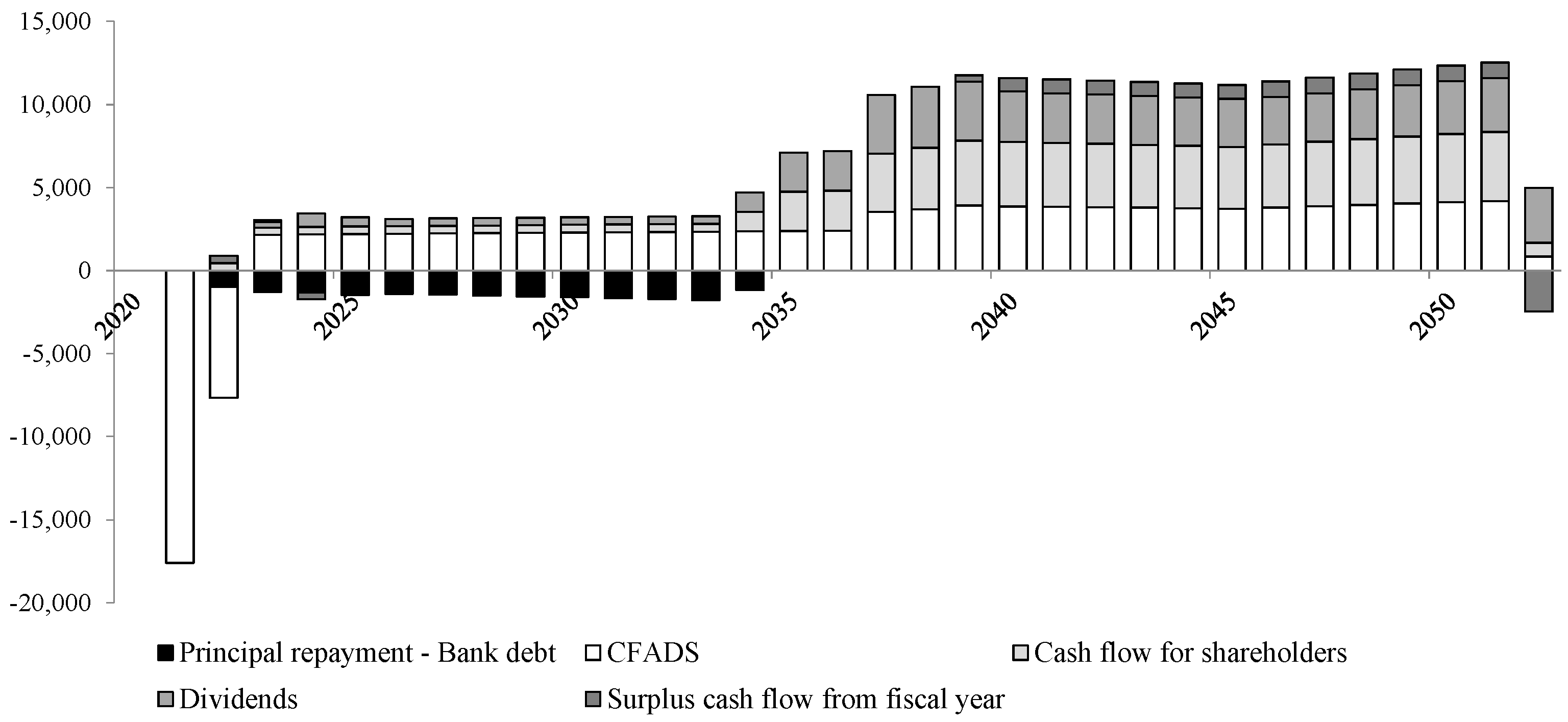
Figure 2 depicts the main items of the cash flow waterfall in Table 5. All projections correspond to the base case, as defined in Table 1 and Table 2. As shown in Table 3, once project construction is completed in 2022, fixed assets amount to 25,371 thousand euros, while bank debt amounts to 18,872 thousand euros (17,777 thousand euros at the end of the year, after debt repayments). As usual in this type of project, the profit and loss accounts in Table 4 show that revenue grows at a steady rate from 2023 onwards, and financial expenses decrease as indebtedness is reduced. Table 3 and Table 4 show that bank charges at the beginning of the project life give rise to deferred taxes amounting to 79 thousand euros in 2021, which reduce the tax burden of the firm in 2022.
Based on the projections shown in Table 5 for equity contributions and the dividends paid to shareholders, Table 6 shows the detail of the calculations used to determine the implied cost of equity of the project considering a time-varying discount rate.
As noted in the previous section, we estimate the risk-free rate in Panels A and B in Table 6 using the Euler approximation of the Vasicek [15] model and one-year Treasury Bill rate data for Spain and UK, respectively, as provided by the OECD Statistics section, for the period from January 1989 to December 2018. We assimilate the long term mean interest rate—b in Expression (3)—to the average Treasury Bill rate for each country in the period 1994–2018. Table 7 shows the regression results provided by the Vasicek [15] model, while 
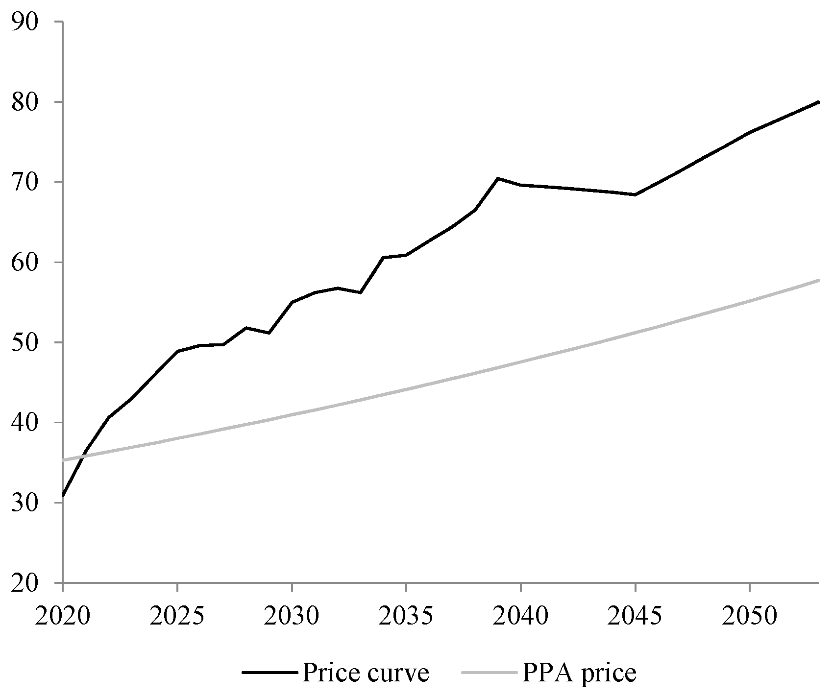
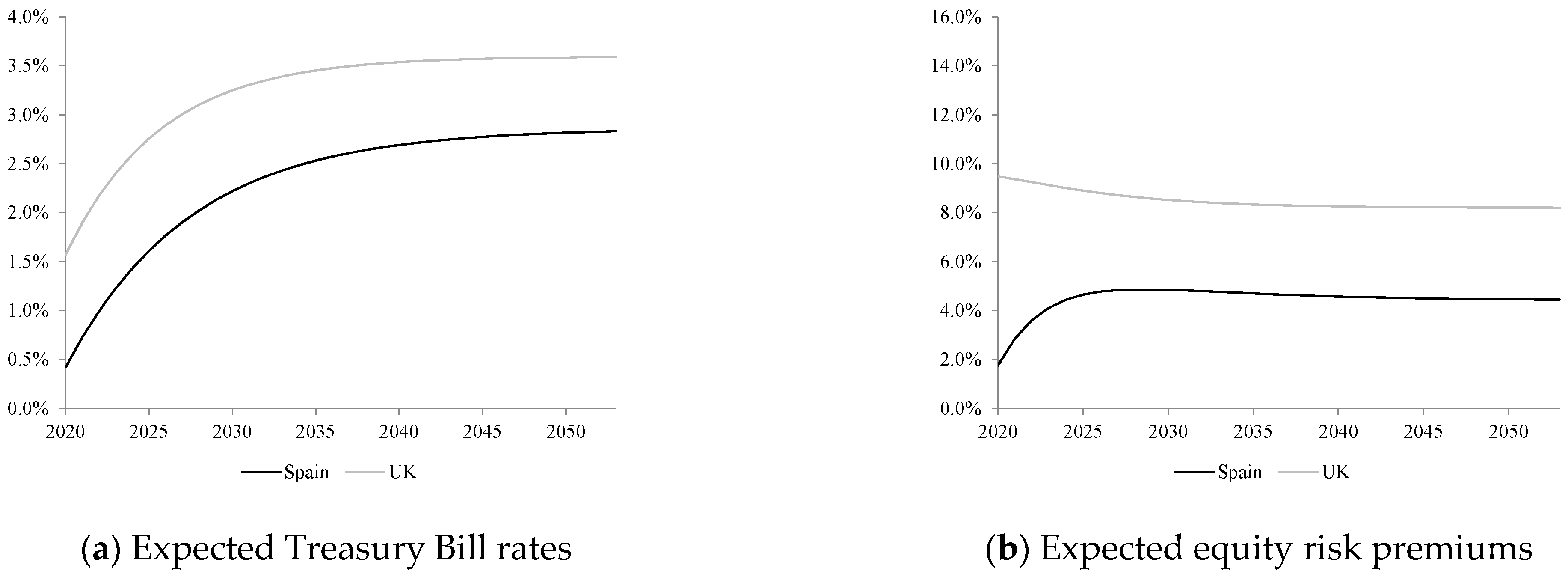
Figure 3a plots the interest rate estimates for Spain and UK, for the period 2020–2053.
To estimate the expected equity risk premium for Spain and UK, we compile return data for all stocks traded on the Madrid Stock Exchange and the London Stock Exchange from the Datastream database, for the period from January 1989 to December 2018. Specifically, we compile the following data series: (i) total return index (RI series), (ii) market value (MV series), and (iii) dividend yield (DY series). Hence, our data series comprise 398 and 4385 stocks for Spain and UK, respectively.
Using these data, we determine the value-weighted market return and the value-weighted dividend yield for the period under consideration. These series allow us to estimate the AR(1) process for the dividend yield and run the forecasting regression defined in Expression (5) (all data are publicly available at [42]). Table 7 shows the regression results for these models, while Figure 3b depicts the expected equity risk premiums that result from Expression (5) for Spain and UK, for the period 2020–2053. Importantly, the estimates in Table 7 show that the dividend yield is highly persistent over time and exhibits a strong predictive power in forecasting the return of the market portfolio, consistently with the results achieved for other countries and markets [43]. Moreover, the predictive power of the dividend yield increases significantly with the horizon, as is often the case with most business cycle predictors (not shown in Table 7).
To estimate beta coefficients, we form two equal-weighed portfolios that allow us to determine the cost of equity for a Spanish and a UK notional investor, respectively. Specifically, these portfolios comprise the following securities: (i) Endesa, S.A. and Iberdrola common stocks, traded on the Madrid Securities Exchange, and (ii) Foresight Solar Fund Ltd. and Bluefield Solar Income Fund Ltd. shares, traded on the London Stock Exchange. Importantly, in order to partially overcome the limitations of the CAPM in determining discount rates, we increase the cost of equity that results from Expression (2) by the alpha coefficients provided by the time-series regressions of portfolio returns on the market portfolio, thus accounting for the pricing errors delivered by the model. Table 8 shows alpha and beta estimates, where unlevered betas are determined using the average equity value, debt and effective tax rate for the companies considered, as provided by the Datastream database, on the Hamada [41] model.
We use the risk-free rates and equity risk premiums in Figure 3, together with alpha and beta estimates in rows labelled ‘Average—Spain’ and ‘Average—UK’ in Table 8, to estimate the time-varying cost of equity of the project for a notional sponsor in Spain or UK, respectively, as shown in Table 6. Specifically, each year we simultaneously determine the equity value and the cost of equity using the equity value itself and the bank debt of the period to estimate the levered betas according to the Hamada [41] model. As a result, the NPV of the project amounts to 1822 thousand euros when we use the cost of equity of a Spanish notional sponsor, and 3057 thousand euros when we use the cost of equity of an UK notional investor, as shown in Panels A and B in Table 6, respectively. To estimate the implied cost of equity throughout the life of the project, we determine the IRR for shareholders that results from subtracting the NPV of the project from the proceeds for shareholders, according to the following expression:
t = 1 T P F S t ( 1 + k e ) t N P V = 0
where P F S t denotes the proceeds for shareholders in the period from t − 1 to t, and k e is the implied cost of equity. Table 6 shows that the implied cost of equity of the Spanish notional sponsor amounts to 10.7%, while it falls to 9.82% for the UK notional investor.
In any case, the results in Table 6 completely ignore the fact that the companies considered to estimate alphas and betas usually invest in turnkey facilities, thus ignoring construction risk. As noted in the previous section, in order to consider the increase in the implied cost of equity that results from construction risk, we use the assumptions shown in Table 1 for the base case and the worst-case scenarios to run a Monte Carlo simulation on the projections shown in Table 3, Table 4 and Table 5. As a result, we obtain a construction risk premium of 2.06%.
To compare the cost of equity of the project with the IRR for shareholders and, consequently, analyse the economic rationale behind the purchase prices paid for ready-to-build solar farms in Spain, Table 9 summarises the main results of our study under different scenarios. Specifically, column I in Table 9 comprises the results achieved for our base case, according to the projections shown in Table 3, Table 4, Table 5 and Table 6. Importantly, while the IRR for shareholders in column I is determined using the proceeds for shareholders shown in Table 6, the IRR for the buyer subtracts a purchase price of 100 € k/MW from the proceeds for shareholders in Table 6, which is consistent with the current prices paid for these transactions in Spain, as noted above. On the other hand, column II in Table 9 comprises the results obtained when we set the production of the solar farm to match the IRR for the buyer to the cost of equity increased by the construction premium. Hence, the required hours of operation should increase from 2200—as considered in the base case—to 2718 for that purpose, as labelled in column II. Finally, columns III and IV in Table 9 show the results of the model when we set the purchase price to match the IRR for the buyer to the cost of equity of a Spanish notional investor (45 € k/MW) and an UK notional investor (78 € k/MW), respectively.
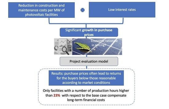
The results in Table 9, column I show that, although the IRR for the shareholders in the base case (12.4%) exceeds the cost of equity for both a Spanish notional investor (10.7%) and an UK notional investor (9.8%) when we ignore the construction risk, if we include the construction premium, the project provides a near-zero NPV, with the cost of equity for a Spanish investor (12.8%) slightly exceeding the IRR for shareholders. However, it should be noted that the cost of equity is clearly above the IRR for the buyer (9.2%) either including or ignoring the construction premium, which suggests that current purchase prices of RTB solar plants are overvalued in the Spanish market. In any case, column I in Table 9 shows that the cost of equity of a UK notional investor amounts to 9.8% when we ignore construction risk, meaning that foreign solar funds can exert upward pressure on purchase prices of solar farms, exploiting their lower cost of equity.
On the other hand, column II in Table 9 shows that the breakeven point of operation hours that equals the IRR for the buyer with the increased cost of equity for both a Spanish notional investor and an UK notional investor amounts to 2718 h, that is, 23.53% more than the number of hours assumed in the base case, which is not easy to achieve under current technological conditions. In this second scenario, the IRR for the buyer amounts to 12.4%, suggesting that the current prices of solar farms are economically viable only for the most efficient parks.
Consistent with the results shown in columns I and II, column III in Table 9 shows that the purchase price that equals the IRR for the buyer with the cost of equity for a Spanish notional investor amounts to 45 € k/MW, that is, 55% less than the purchase price assumed in the base case. On the other hand, the lower cost of equity of UK solar funds allows these investment vehicles to reach a purchase price of 78 € k/MW. In any case, it should be noted that the production assumed in the base case (2200 h) prevents the project from providing an IRR for the buyer that simultaneously compensates for the cost of equity and the construction premium.

4. Conclusions

Based on updated data from the Spanish renewable energy market in early 2020, and using return data from both the Spanish and the UK equity markets to determine conditional discount rates, the forecasts shown in the previous section for a generic photovoltaic plant located in Spain provide us with three major findings. First, although the expected IRR for shareholders largely compensates for the implied cost of equity that results from conditional discount rates both ignoring and including construction risks, prices paid at the valuation date for RTB facilities translate into an IRR for the buyer that is clearly below the implied cost of equity. Consistent with previous literature on the topic [11,12,13,14], these results suggest that, although Spanish RTB photovoltaic plants provide on average a near-zero NPV for shareholders, the NPV for buyers paying purchase prices equal to or greater than 100 € k/MW for these facilities—as is often the case at the valuation date—is likely to fall below zero, which is consistent with an apparent overvaluation of the market.
Second, on average, the purchase prices paid at the valuation date for RTB photovoltaic plants only compensate the implied cost of equity in the case of the most efficient projects. In particular, our results show that only facilities that exceed a production of 2718 h—that is, 23.53% more than the number of hours considered in the base case—provide an IRR for shareholders that compensate the cost of equity. That production translates into an IRR for shareholders equal to 16.4% (see column II in Table 9), which would realistically require not only an increase in production hours, but also a further decrease of investment and operation costs. Remarkably, for that number of hours, both the IRR for the buyer and the implied cost of equity amount to 12.4%.
Third, notwithstanding the above, specialised investors, such as international investment vehicles investing in projects globally, can exploit their lower cost of equity to pay prices significantly higher than those affordable by domestic investors in non-financial industries. Specifically, our results show that, while the purchase price that allows large domestic utilities to compensate their cost of equity amounts to 45 € k/MW, this price rises to 78 € k/MW in the case of UK solar funds, that is, 73.33% higher. These results suggest that specialised international investors can exert upward pressure on purchase prices of solar plants, exploiting their lower cost of equity.

Author Contributions

Conceptualisation, M.V.-V., A.B.A.-C. and J.R.-S.; methodology, M.V.-V., A.B.A.-C. and J.R.-S.; software, M.V.-V., A.B.A.-C. and J.R.-S.; validation, M.V.-V., A.B.A.-C. and J.R.-S.; formal analysis, M.V.-V., A.B.A.-C. and J.R.-S.; investigation, M.V.-V., A.B.A.-C. and J.R.-S.; resources, M.V.-V., A.B.A.-C. and J.R.-S.; data curation, M.V.-V., A.B.A.-C. and J.R.-S.; writing—original draft preparation, M.V.-V., A.B.A.-C. and J.R.-S.; writing—review and editing, M.V.-V., A.B.A.-C. and J.R.-S.; visualisation, M.V.-V., A.B.A.-C. and J.R.-S.; supervision, M.V.-V., A.B.A.-C. and J.R.-S.; project administration, A.B.A.-C. and J.R.-S. All authors have read and agreed to the published version of the manuscript.

Funding

This research was funded by the Education and Research Service of the Madrid regional government and the European Social Fund, grant numbers PEJD-2017-PRE/SOC-4289 and PEJD-2018-PRE/SOC-8898.

Institutional Review Board Statement

Not applicable.

Informed Consent Statement

Not applicable.

Data Availability Statement

All data used in discount rate estimation are publicly available at Vázquez-Vázquez, M.; Alonso-Conde, A.B.; Rojo-Suárez, J. Data for: Are the purchase prices of solar energy projects under development consistent with cost of capital forecasts? 2021, http://0-dx-doi-org.brum.beds.ac.uk/10.17632/2zfwxw2z2f.3 (accessed on 17 May 2021).

Conflicts of Interest

The authors declare no conflict of interest.

References

  1. Lin, B.; Xu, B. How to Promote the Growth of New Energy Industry at Different Stages? Energy Policy 2018, 118, 390–403. [Google Scholar] [CrossRef]
  2. Zeng, S.; Jiang, C.; Ma, C.; Su, B. Investment Efficiency of the New Energy Industry in China. Energy Econ. 2018, 70, 536–544. [Google Scholar] [CrossRef]
  3. Ye, P.; Li, Y.; Zhang, H.; Shen, H. Bibliometric Analysis on the Research of Offshore Wind Power Based on Web of Science. Econ. Res. Ekon. Istraživanja 2020, 33, 887–903. [Google Scholar] [CrossRef] [Green Version]
  4. Azam, A.; Rafiq, M.; Shafique, M.; Yuan, J. Renewable Electricity Generation and Economic Growth Nexus in Developing Countries: An ARDL Approach. Econ. Res. Ekon. Istraživanja 2021, 1–24. [Google Scholar] [CrossRef]
  5. Machete, I.; Marques, R. Financing the Water and Sanitation Sectors: A Hybrid Literature Review. Infrastructures 2021, 6, 9. [Google Scholar] [CrossRef]
  6. OECD. Investing in Climate, Investing in Growth; OECD Publishing: Oxford, UK, 2017. [Google Scholar]
  7. Holden, P.B.; Edwards, N.R.; Ridgwell, A.; Wilkinson, R.D.; Fraedrich, K.; Lunkeit, F.; Pollitt, H.; Mercure, J.F.; Salas, P.; Lam, A.; et al. Climate–Carbon Cycle Uncertainties and the Paris Agreement. Nat. Clim. Chang. 2018, 8, 609–613. [Google Scholar] [CrossRef]
  8. Gabteni, H.g.; Bami, A. Energy Transition: Between Economic Opportunity and the Need for Financing? Int. J. Glob. Energy Issues 2018, 41, 146–157. [Google Scholar] [CrossRef]
  9. REN21. Renewables 2019 Global Status Report; Renewable Energy Policy Network for the 21st Century: Paris, France, 2019. [Google Scholar]
  10. REE. Las Energías Renovables en el Sistema Eléctrico Español; Red Eléctrica de España: Madrid, Spain, 2019. [Google Scholar]
  11. Bohl, M.T.; Kaufmann, P.; Stephan, P.M. From Hero to Zero: Evidence of Performance Reversal and Speculative Bubbles in German Renewable Energy Stocks. Energy Econ. 2013, 37, 40–51. [Google Scholar] [CrossRef] [Green Version]
  12. Wang, K.-H.; Su, C.-W.; Lobonţ, O.-R.; Moldovan, N.-C. Chinese Renewable Energy Industries’ Boom and Recession: Evidence from Bubble Detection Procedure. Energy Policy 2020, 138, 111200. [Google Scholar] [CrossRef]
  13. Semieniuk, G.; Campiglio, E.; Mercure, J.-F.; Volz, U.; Edwards, N.R. Low-Carbon Transition Risks for Finance. Wires Clim. Chang. 2021, 12, e678. [Google Scholar] [CrossRef]
  14. Martín, H.; Coronas, S.; Alonso, À.; de la Hoz, J.; Matas, J. Renewable Energy Auction Prices: Near Subsidy-Free? Energies 2020, 13, 3383. [Google Scholar] [CrossRef]
  15. Vasicek, O. An Equilibrium Characterization of the Term Structure. J. Financ. Econ. 1977, 5, 177–188. [Google Scholar] [CrossRef]
  16. Campbell, J.Y.; Shiller, R.J. The Dividend-Price Ratio and Expectations of Future Dividends and Discount Factors. Rev. Financ. Stud. 1988, 1, 195–228. [Google Scholar] [CrossRef] [Green Version]
  17. Mendicino, L.; Menniti, D.; Pinnarelli, A.; Sorrentino, N. Corporate Power Purchase Agreement: Formulation of the Related Levelized Cost of Energy and its Application to a Real Life Case Study. Appl. Energy 2019, 253, 113577. [Google Scholar] [CrossRef]
  18. Servert, J.F.; Cerrajero, E.; Fuentealba, E.L.; Greos, S. Feasibility of a CSP Power Plant in Chile under a PPA Model, the Role of Soft Financing and Upfront Grant. Energy Procedia 2015, 69, 1704–1710. [Google Scholar] [CrossRef] [Green Version]
  19. Miller, L.; Carriveau, R.; Harper, S.; Singh, S. Evaluating the Link between LCOE and PPA Elements and Structure for Wind Energy. Energy Strategy Rev. 2017, 16, 33–42. [Google Scholar] [CrossRef]
  20. BloombergNEF. 1H 2020 European Corporate PPA Price Survey; BloombergNEF: Hong Kong, 2020. [Google Scholar]
  21. Tegen, S.; Hand, M.; Maples, B.; Lantz, E.; Schwabe, P.; Smith, A. Cost of Wind Energy Review; National Renewable Energy Laboratory: Golden, CO, USA, 2013.
  22. Giberson, M. Assessing Wind Power Cost Estimates; Institute for Energy Research: Washington, DC, USA, 2013. [Google Scholar]
  23. IRENA. Renewable Power Generation Costs in 2019; International Renewable Energy Agency: Abu Dhabi, United Arab Emirates, 2020. [Google Scholar]
  24. Ng, T.H.; Tao, J.Y. Bond Financing for Renewable Energy in Asia. Energy Policy 2016, 95, 509–517. [Google Scholar] [CrossRef] [Green Version]
  25. MacAskill, S.; Roca, E.; Liu, B.; Stewart, R.A.; Sahin, O. Is There a Green Premium in the Green Bond Market? Systematic Literature Review Revealing Premium Determinants. J. Clean. Prod. 2021, 280, 124491. [Google Scholar] [CrossRef]
  26. Alonso-Conde, A.-B.; Rojo-Suárez, J. On the Effect of Green Bonds on the Profitability and Credit Quality of Project Financing. Sustainability 2020, 12, 6695. [Google Scholar] [CrossRef]
  27. Vassallo, J.M.; Rangel, T.; Baeza, M.d.l.Á.; Bueno, P.C. The Europe 2020 Project Bond Initiative: An Alternative to Finance Infrastructure in Europe. Technol. Econ. Dev. Econ. 2018, 24, 229–252. [Google Scholar] [CrossRef] [Green Version]
  28. Alonso-Conde, A.B.; Rojo-Suárez, J. Modelos de Estimación de Ingresos en Empresas de Internet. Investig. Eur. Dir. Econ. Empresa (IEDEE) 2005, 11, 27–43. [Google Scholar]
  29. Gonzalez-Ruiz, J.D.; Peña, A.; Duque, E.A.; Patiño, A.; Chiclana, F.; Góngora, M. Stochastic logistic fuzzy maps for the construction of integrated multirates scenarios in the financing of infrastructure projects. Appl. Soft Comput. 2019, 85, 105818. [Google Scholar] [CrossRef]
  30. Sharpe, W.F. Capital Asset Prices: A Theory of Market Equilibrium under Conditions of Risk. J. Financ. 1964, 19, 425–442. [Google Scholar] [CrossRef] [Green Version]
  31. Lintner, J. The Valuation of Risk Assets and the Selection of Risky Investments in Stock Portfolios and Capital Budgets. Rev. Econ. Stat. 1965, 47, 13–37. [Google Scholar] [CrossRef]
  32. Lintner, J. Security Prices, Risk, and Maximal Gains from Diversification. J. Financ. 1965, 20, 587–615. [Google Scholar] [CrossRef]
  33. Jagannathan, R.; Wang, Z. The Conditional CAPM and the Cross-Section of Expected Returns. J. Financ. 1996, 51, 3–53. [Google Scholar] [CrossRef]
  34. Lettau, M.; Ludvigson, S. Resurrecting the (C)CAPM: A Cross-Sectional Test When Risk Premia Are Time-Varying. J. Polit. Econ. 2001, 109, 1238–1287. [Google Scholar] [CrossRef] [Green Version]
  35. Maio, P.; Santa-Clara, P. Multifactor Models and their Consistency with the ICAPM. J. Financ. Econ. 2012, 106, 586–613. [Google Scholar] [CrossRef]
  36. Campbell, J.Y.; Giglio, S.; Polk, C.; Turley, R. An Intertemporal CAPM with Stochastic Volatility. J. Financ. Econ. 2018, 128, 207–233. [Google Scholar] [CrossRef] [Green Version]
  37. Shiller, R.J. Do Stock Prices Move Too Much to be Justified by Subsequent Changes in Dividends? Am. Econ. Rev. 1981, 71, 421–436. [Google Scholar]
  38. Fama, E.F.; French, K.R. Dividend Yields and Expected Stock Returns. J. Financ. Econ. 1988, 22, 3–25. [Google Scholar] [CrossRef]
  39. Cochrane, J.H. A Cross-Sectional Test of an Investment-Based Asset Pricing Model. J. Polit. Econ. 1996, 104, 572–621. [Google Scholar] [CrossRef]
  40. Ferson, W.E.; Schadt, R.W. Measuring Fund Strategy and Performance in Changing Economic Conditions. J. Financ. 1996, 51, 425–461. [Google Scholar] [CrossRef]
  41. Hamada, R.S. The Effect of the Firm’s Capital Structure on the Systematic Risk of Common Stocks. J. Financ. 1972, 27, 435–452. [Google Scholar] [CrossRef]
  42. Vázquez-Vázquez, M.; Alonso-Conde, A.B.; Rojo-Suárez, J. Data for: Are the Purchase Prices of Solar Energy Projects under Development Consistent with Cost of Capital Forecasts? 2021. Available online: https://data.mendeley.com/datasets/2zfwxw2z2f/2 (accessed on 17 May 2021).
  43. Cochrane, J.H. Presidential Address: Discount Rates. J. Financ. 2011, 66, 1047–1108. [Google Scholar] [CrossRef] [Green Version]
Figure 1. Expected solar price curve and PPA prices.
Infrastructures 06 00095 g001
Figure 2. Main aggregates of the cash flow waterfall for the base case.
Infrastructures 06 00095 g002
Figure 3. Expected Treasury Bill rates and equity risk premiums.
Infrastructures 06 00095 g003
Table 1. Operational assumptions.
ItemUnitsBase CaseWorst Case
Panel A: General assumptions
Purchase price€ k40004000
Purchase price/MW€ k/MW100.00100.00
ProductionHours2200.002200.00
MW peakMW45.0045.00
MW nominalMW40.0040.00
Capacity%90.00%90.00%
Degradation%0.10%0.10%
Panel B: Timing
Valuation dateDate1 January 20201 January 2020
Start of the constructionDate1 September 20211 September 2021
Construction periodMonths612
Commercial operation date—StartDate1 March 20221 September 2022
Commercial operation date—EndDate1 March 20521 September 2052
Panel C: CapEx and depreciation
Industrial CapEx€ k/MW580816
Industrial CapEx€ k26,10036,720
Depreciation periodYears3030
Panel D: OpEx
O&M expenses€ k/MW13.2513.25
O&M expenses€ k/year596596
Inflation O&M expenses%1.50%1.50%
Panel E: Working capital
Collection periodDays15.0015.00
Payment periodDays30.0030.00
Table 2. Financial assumptions.
ItemUnitsValue
Panel A: Funding
% Bank loan%70.00%
% Shareholders%30.00%
Panel B: Interest rates and commissions of debt
Bank loan—Interest rate%2.50%
Bank loan—Upfront fee%1.80%
Panel C: Debt repayment
Term of debtYears15
Debt service coverage ratioUnits1.25
Table 3. Pro forma balance sheet for the base case.
2020202120222023202420252026205020512052
Total non-current assets-17,67225,37124,50123,63122,76121,891 1011141-
Fixed assets-17,59225,37124,50123,63122,76121,891 1011141-
Deferred taxes-79----- ---
Total current assets--556653264139141 10,40411,3368634
Accounts receivable--112135137139141 27127546
Cash--444517127-- 10,13311,0608588
Total assets-17,67225,92725,15323,89422,90022,032 11,41511,4768634
Shareholders’ equity-520384078876892792599767 11,30011,3608615
Capital-544180498049804980498049 804980498049
Reserves--(238)--309764 ---
Profit and loss account-(238)596827877900953 32513311565
Liabilities-12,46817,52016,27714,96813,64112,265 11511620
Bank loan-12,69717,77716,50015,16713,81712,417 ---
Bank loan—Upfront fee-(229)(316)(293)(270)(248)(225) ---
Accounts payable--5870717273 11511620
Total equity and liabilities-17,67225,92725,15323,89422,90022,032 11,41511,4768634
Table 4. Pro forma profit and loss statement for the base case.
2020202120222023202420252026205020512052
Revenue--27213293334133903436 659966991133
Operating expenses--(515)(623)(633)(642)(652) (932)(946)(160)
Power generation taxes--(190)(231)(234)(237)(241) (462)(469)(79)
EBITDA--20162439247525102544 52055284894
Depreciation--(729)(870)(870)(870)(870) (870)(870)(141)
EBIT--12861569160516401674 43354414753
Financial expenses -(317)(470)(444)(412)(417)(380) ---
Upfront fee amortisation--(23)(23)(23)(23)(23) ---
Income before taxes-(317)7941102117012011271 43354414753
Income taxes-79(199)(276)(292)(300)(318) (1084)(1104)(188)
Net income-(238)596827877900953 32513311565
Table 5. Cash flow waterfall for the base case.
2020202120222023202420252026205020512052
Revenue--27213293334133903436 659966991133
Operating expenses--(705)(854)(867)(880)(893) (1394)(1415)(239)
Income taxes--(119)(276)(292)(300)(318) (1084)(1104)(188)
CapEx-(17,592)(8508)---- ---
Changes in working capital--(54)(11)(1)(1)(1) (3)(2)132
CFADS-(17,592)(6665)2152218222092225 41184178838
Financial expenses-(317)(470)(444)(412)(417)(380) ---
Commissions-(229)(110)---- ---
Principal repayment --(1005)(1277)(1333)(1350)(1400) ---
Cash flow after debt service-(18,138)(8249)430436442445 41184178838
Contributions—Capital-54412608---- ---
Contributions—Bank debt-12,6976085---- ---
Cash flow for shareholders--444430436442445 41184178838
Dividends---(358)(827)(569)(445) (3170)(3251)(3311)
Capital reimbursement------- ---
Surplus cash flow--44473(390)(127)- 948927(2473)
Table 6. Equity valuation and implied cost of equity for the base case.
2020202120222023202420252026205020512052
Proceeds for shareholders(0)(5441)(2608)358827569445 325133118615
Bank debt-12,69717,77716,50015,16713,81712,417 ---
Panel A: Spanish sponsor
Risk-free rate0.42%0.73%1.00%1.23%1.43%1.61%1.77% 2.82%2.83%
Equity risk premium1.75%2.86%3.61%4.11%4.44%4.65%4.77% 4.45%4.45%
Levered beta0.26430.60400.59300.54990.51840.48280.4472 0.26430.2643
Cost of equity: Impl. ke 10.70%7.91%9.48%10.16%10.52%10.76%10.88%10.93% 11.03%11.03%
Equity value1822740710,71711,44911,82612,53013,449 99707759
Panel B: UK sponsor
Risk-free rate1.58%1.90%2.18%2.41%2.60%2.76%2.89% 3.59%3.59%
Equity risk premium9.48%9.37%9.25%9.12%9.01%8.90%8.80% 8.21%8.20%
Levered beta−0.3058−0.6375−0.6468−0.6108−0.5841−0.5511−0.5157 −0.3058−0.3058
Cost of equity: Impl. ke 9.82%9.25%6.50%6.77%7.41%7.91%8.43%8.93% 11.65%11.65%
Equity value3057878211,96112,41212,50512,92513,569 98757715
Table 7. Forecasting regressions.
Panel A: Spain
RfDPRm
Slope−0.1250.7244.296
(0.043)(0.140)(3.360)
t-statistic−2.8795.1741.279
R20.2280.4980.057
Panel B: UK
RfDPRm
Slope−0.1610.71211.474
(0.058)(0.129)(4.170)
t-statistic−2.7725.4972.752
R20.2150.5280.219
1 The table shows the regression results of the following models: (i) the discrete version of the Vasicek (1977) model R t f = a ( b R t f ) + ε t , where a is the speed of reversion of the current interest rate to its long-term mean level, and b is long-term mean interest rate, (ii) the AR(1) process of the dividend yield D P t = a + b D P t 1 + ε t , and (iii) the forecasting regression of the market return on the lagged weighted average dividend yield, R t m = a + b D P t 1 + ε t , consistent with Expression (5). Standard errors are in parentheses.
Table 8. Alpha and unlevered beta estimates.
BenchmarkCountryAlphaUnlevered Beta
Average—SpainSpain7.03%26.43%
Average—UKUK10.57%−30.58%
Endesa, S.A.Spain7.63%37.64%
Iberdrola, S.A.Spain6.43%20.98%
Foresight Solar Fund Ltd.UK8.40%−24.26%
Bluefield Solar Income Fund Ltd.UK12.75%−36.91%
Table 9. IRR for shareholders and cost of equity.
ColumnIIIIIIIV
Price: 100 € k/MWPrice: 100 € k/MWPrice: 45 € k/MWPrice: 78 € k/MW
Prod.: 2200 hProd.: 2718 hProd.: 2200 hProd.: 2200 h
IRR for sh.12.4%16.4%12.4%12.4%
IRR for sh.—Buyer9.2%12.4%10.7%9.8%
ke Spain10.7%10.4%10.7%10.7%
ke Spain + Constr. prem.12.8%12.4%12.8%12.8%
ke UK9.8%10.4%9.8%9.8%
ke UK + Constr. prem.11.9%12.4%11.9%11.9%
Publisher’s Note: MDPI stays neutral with regard to jurisdictional claims in published maps and institutional affiliations.

