1. Introduction
Karst geomorphology in the world is produced by dissolution of carbonate rocks, developing surface characteristics as poljes, sinkholes (dolines), shallow holes and it is through these voids or conduits that groundwater can flow [
1]. The karst landscape is part of the 20% of the area in the earth [
2] and according to Conrado-Palafox [
3], the karst activity has a high influence on the stresses in the ground that produces settlements on the terrain. The settlement represents a handicap in the road design and in its structural performance as well as in other constructions.
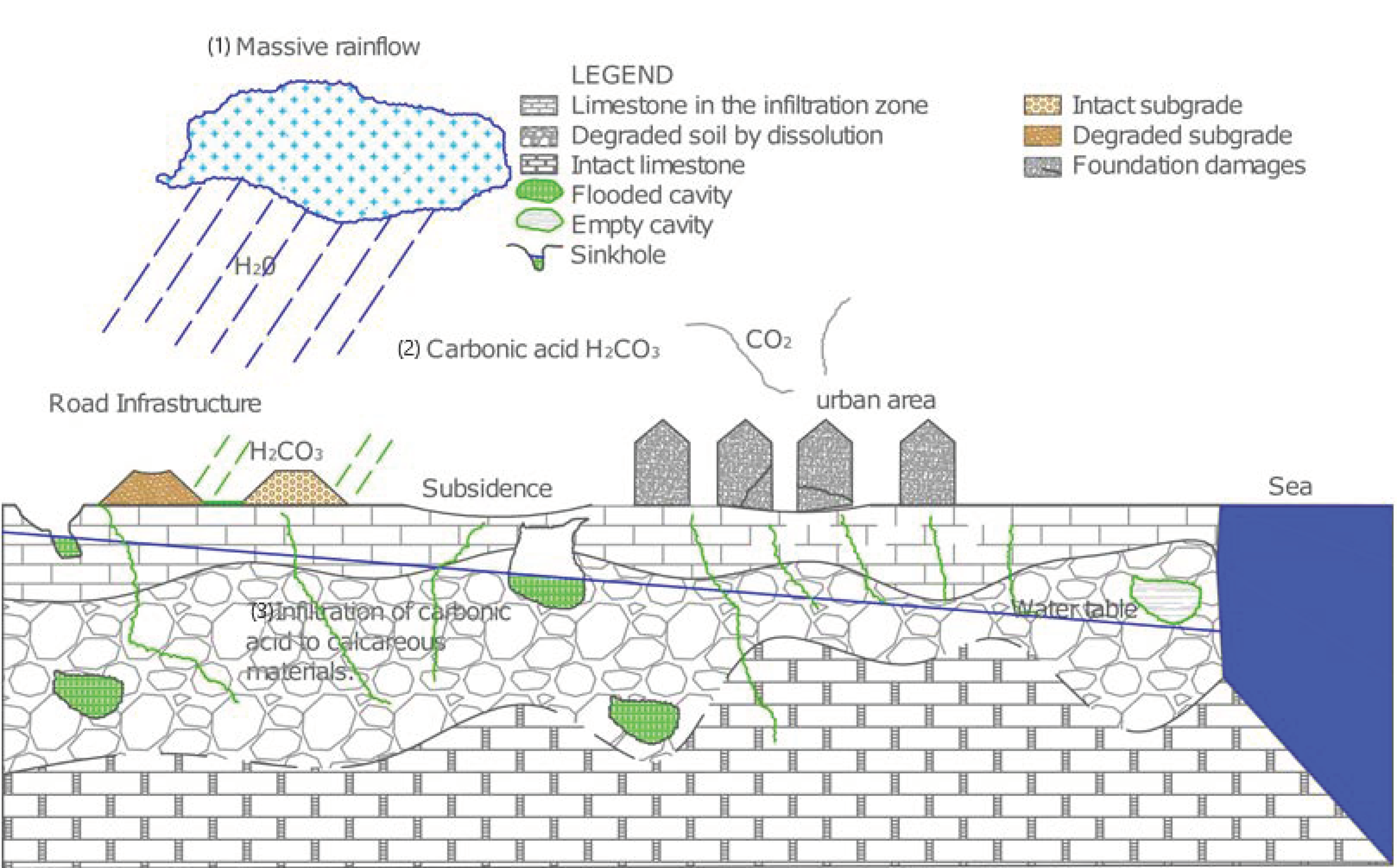
In the specific case of Yucatan, Mexico, the karst phenomena have been investigated several occasions and it was pointed out that its formation is very complex and where several non-traditional factors intervene [
4,
5]. Furthermore, Springall [
6] explained that the biggest dissolution area is located in the first meters of subsoil and Bauer-Gottwein [
7] mentions that there are several caves with 2.0 m diameter less than 15 m deep (
Figure 1).
Determining the specific location of the cavities in Yucatan is not easy, because the dolines density is variable, and they are located in random points in the entire Yucatan region [
8]. Therefore, there are several studies about the mapping karst system [
9,
10,
11,
12] that can be used in construction, nevertheless, Bonacci [
13] established that industrial development in particular regions, such as water pumping causes redistribution in karst catchments, which strongly and dangerously affects processes of water circulation and weathering. The city of Merida, Yucatan, concentrates 50% of the population in 2% of the State area and most of the industries are also located on the outskirts of the capital, the demographic and economic growth in Yucatan peninsula in recent years have caused changes in the hydrological response and flow of water cycle, due to the increase in water consumption but with a 23% decrease in groundwater recharge [
14]. It is important to describe the water balance because, although the solubility of limestone in pure water is extremely low [
15], the CO
2 emissions from human activities such as urbanization, stone clearing, quarrying, and deforestation accelerate the weathering in the karst landscape [
16,
17].
The high frequency of mechanical failure in karst terrains is primarily due to the low strength of the young limestone. Therefore, collapse is an inevitable consequence of the excessive tensile stresses as result of the geo-material dissolution [
18]. The mechanical failures have been treated by applying several methods, such as concrete injection through the boreholes [
19], however, this can cause differential settlements related to the isolated impermeable material and contribute to the change of the local hydrogeological condition [
20].
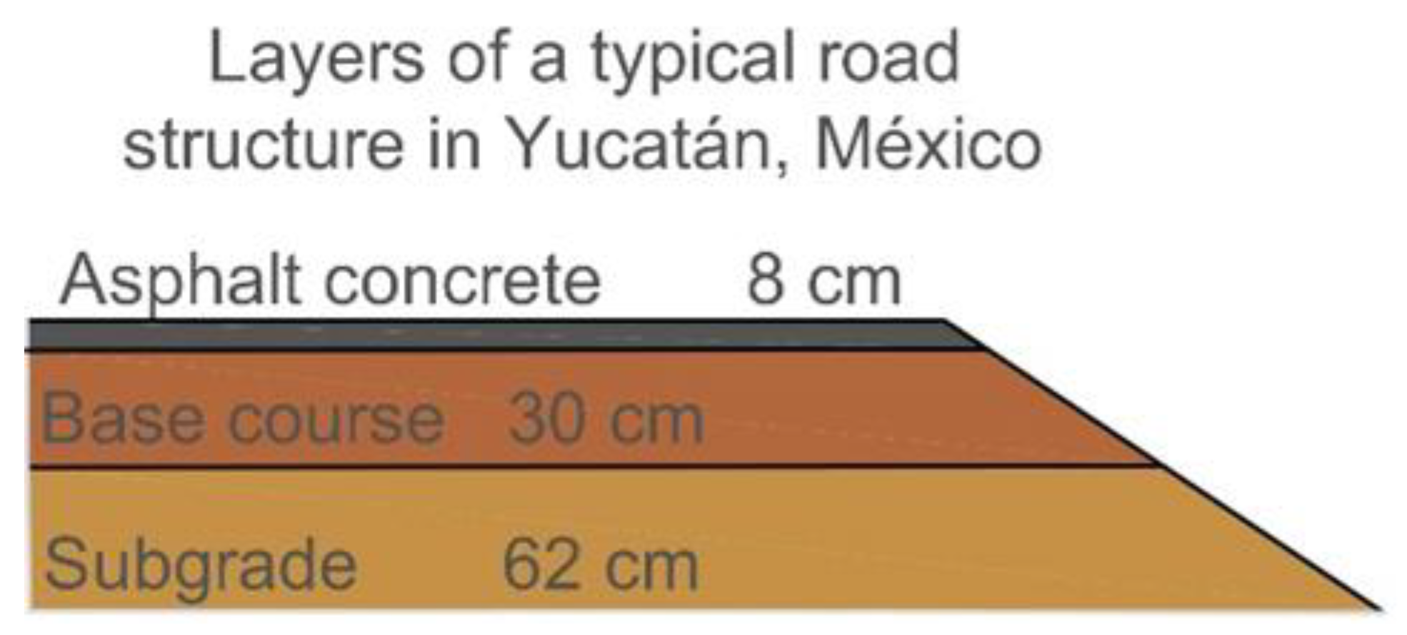
The typical road structure constructed in Yucatan is shown in
Figure 2. The road thickness is thin because of the Yucatecan flat rock platform, and although the section has had good performance over the limestone platform, the road suffers a differential displacement on account of the presence of a cavity as is found by Gutiérrez [
21] and Saenseela [
22].
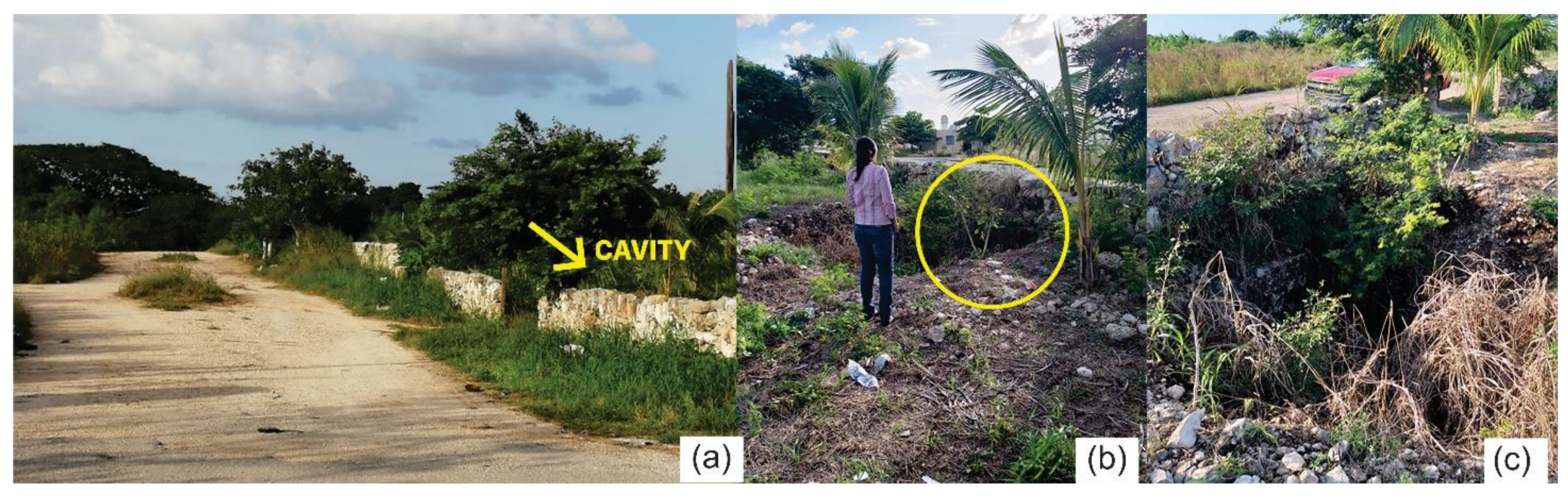
Figure 3a shows an example of the soil surface in Merida, Mexico, and
Figure 3b,c show a cavity next to a road. In those it is possible to observe one effect of the karst activity and although the effect and the problematic is evident, Yucatan road Standard does not consider an alternative to avoid the karst effect.
In this way, this study is focused in proposing a solution for the road problems caused by the karsticity phenomena, considering a typical road structure as established in the Mexican Normative [
23] and considering the geogrid inclusions in design, through the improvement observed and according to the numerical results presented in this work.
2. Background of Reinforcements with Geogrids
Geogrids are an economic solution for road problems in soils with poor bearing capacity [
24,
25,
26,
27] or for reducing the rutting damage in base course and subgrade layers [
28]. In the way to find solutions, several numerical methods have been developed to analyze geogrids improvement and some of these conclude that the use of one geogrid layer or two of them increase the bearing capacity of the soil, because of the well distributed stresses along of the geogrids [
29]. Railway design is another infrastructure that uses the numerical methods to analyze the use of geogrids, such as Jiang [
30] that established the ballast/sub-ballast interface as the optimum geogrid placement location and the improvement is more notorious when there is a poor subgrade than a rigid one. Similarly, Ngo [
31], concluded that the use of geogrid reduces ballast dilatation carrying out discrete element method and physical laboratory test.
Recent studies have explored the mitigation of a road structure over only one void such as Wang [
32], who carried out a finite element modelling of an embankment over a large sinkhole and concluded that the geosynthetic has a more significant influence on the settlement at the base of the embankment than in the crest, it should be noted that this investigation also add drilled shafts as a road improvement and the layer under the embankment was a silty clay. Moreover, Sireesh [
33] concluded with laboratory scale model tests that a geocell reinforced sand over clay bed with a circular void is an excellent reinforcement to increase the bearing capacity and reduce settlement of the clay subgrade. Finally, Galve [
34] points out the profitable use of geosynthetics in road structures to mitigate the extra cost due to cavity damages, based on probabilistic methodology and sinkholes area data and cos-benefit analysis.
Under these statements, an option to improve the strength and mechanical properties of soil is to introduce a geogrid as a reinforcement surface element. However, there are few investigations about the improvement of the geogrids in karst terrains or investigations of preventing road settlement problems when the subsoil has a subsidence problem due to the weathering effect of the material, furthermore, most studies in the field have only focused on clay sublayers and with only one cavity in the model. This study provides new insight into road reinforcement with geogrids but considering several voids in the terrain and pointing out the best position of a geogrid layer in the road structure in order to mitigate road failures due to the subsidence in the terrain caused by many cavities.
3. Material and Methods
The objective of the numerical analyses in PLAXIS
® [
35] is to determine the better position and the combination of the geogrids placed under different layers of the road structure studied (see
Figure 2). Obtained results were analyzed in function of the capacity of mitigation of the soil failure and the effect of the presence of several cavities in the ground, being this part the main handicap in the analyzed zone, because as described in [
36] the Yucatan karst landscape is characterized for having several small holes in the subsoil, as can be seen in Figure 5.
The numerical modelling was based on the conceptual flow chart showed in
Figure 4. Firstly, the input parameters were stablished such as the size of the model with the length of each layer (granular soil and rock layer), the boundary conditions and the geometry and positions of each of the 19 cavities. Secondly, the road structure was added in the model placing a geogrid layer between each layer, at the end one of the cases analyzed in this study had 4 geogrids layer and other cases had only 1 geogrid in the bottom and/or in the crest of the road. Once the road reinforcement structure was completed, the static truck load was applied over the asphalt layer. The methodology of opening and creating the cavities in the finite element model was obtained from Conrado-Palafox [
3]. In the following section each step of the flow chart is explained more in detail.
3.1. Numerical Modelling
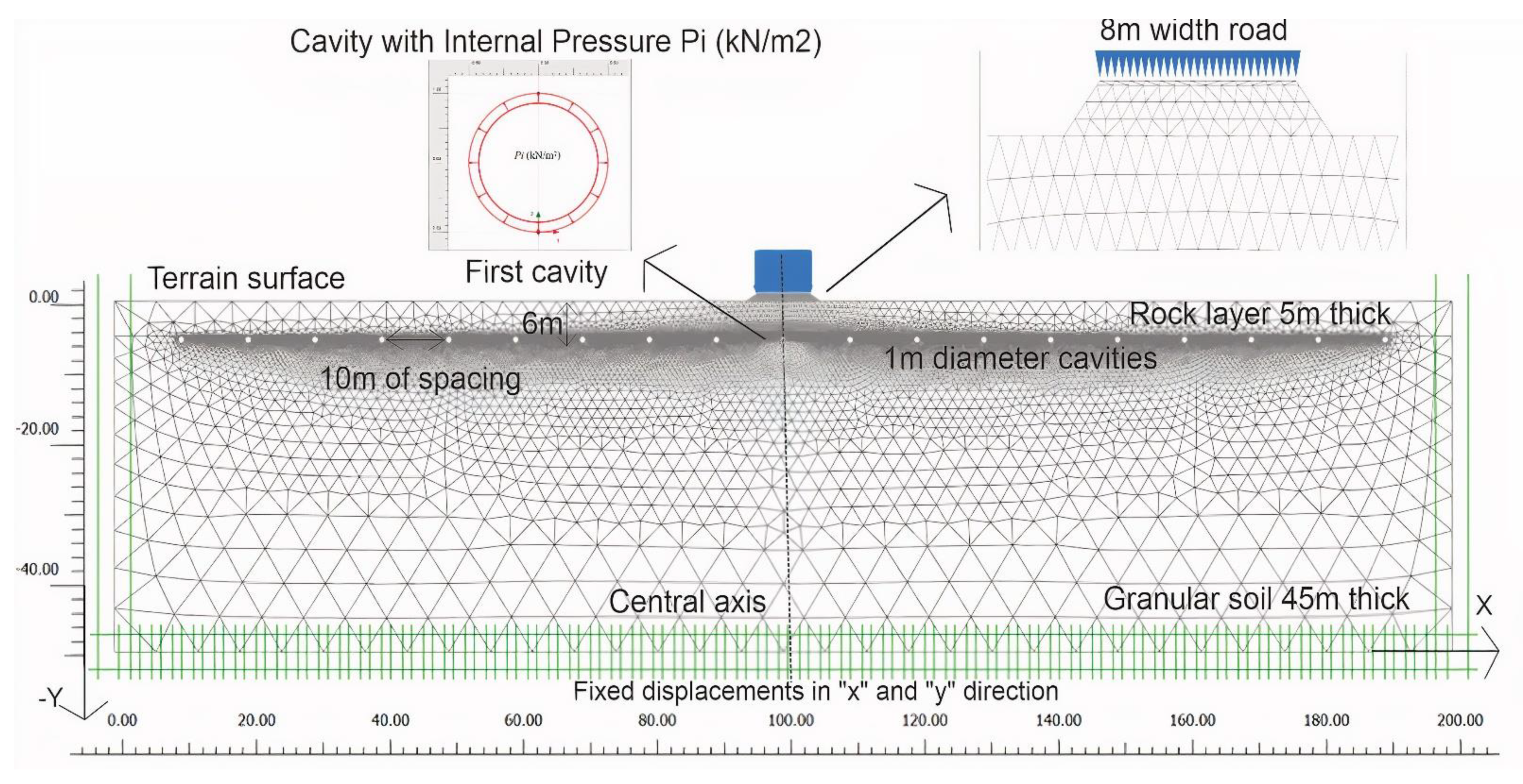
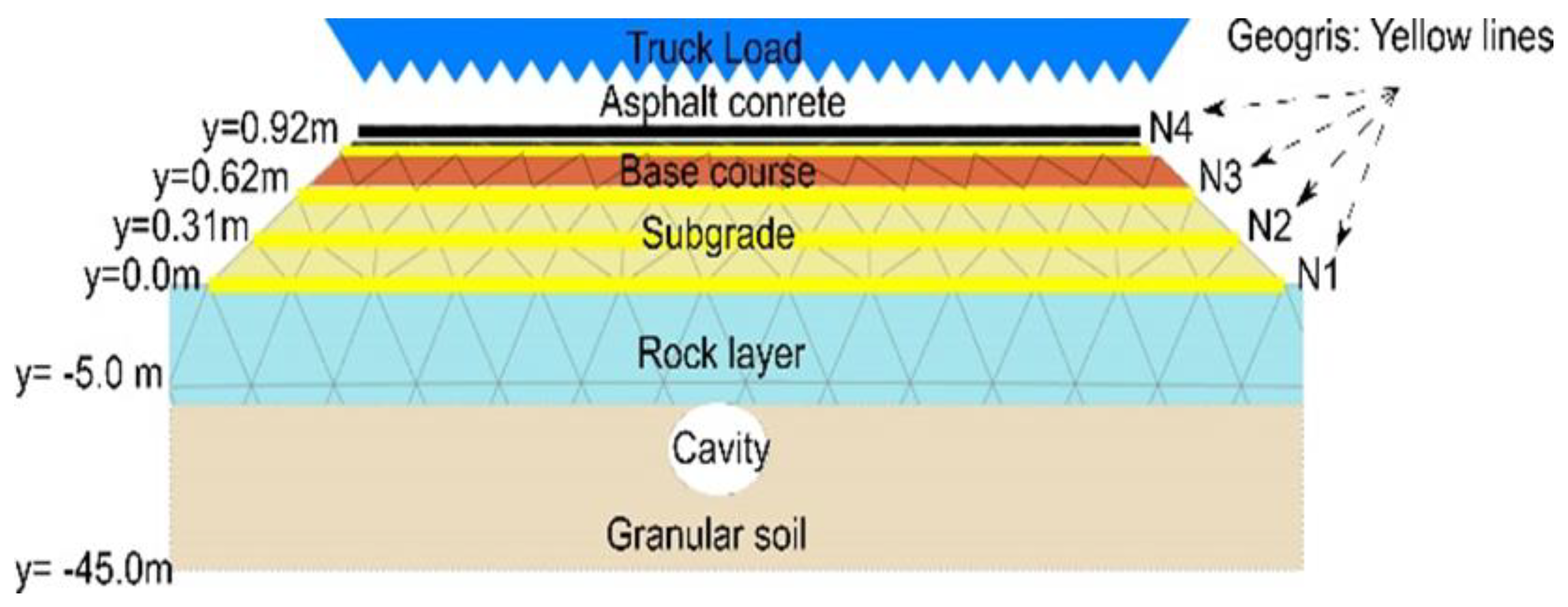
The geometry of the plane strain (2D) model is 200 m × 50 m to avoid numerical errors and the boundary considerations are: the bottom is defined by the restriction of movements on the x-axis (horizontal) and y-axis (vertical), whereas on the vertical sides only x-axis was restricted as is showed in
Figure 5. Over the terrain, the road structure with 11 m base and 8 m roadway was laid.
Figure 6 illustrates the numerical model soil layers, the geogrid position
N1,
N2,
N3 and
N4, the truck load and the nomenclature used.
The numerical modelisation was generalized in four principal “Phases” as is exemplified in
Table 1. In the “Initial phase”, the stratigraphy composed by a rock layer and granular soil was modeled and then, the road structure considering its own weight (Road structure phase) was created to in the third Phase (Phase of the Static load) apply the heavy truck load (4.84 kN/m
2) [
37].
The last Phase named “Cavities” was developed in 10 different steps to simulate the karst evolution and the cavities were placed under the rock layer in the model as is schematized in
Figure 5. The first step of this Phase start with one 1-m diameter cavity at the mid of the numerical model (see
Figure 6) and in the next 9 steps, it was added two cavities in each one, until the 18 cavities were symmetrically created. Although the road seems to be influenced only by three cavities it was important to study the effect of the other cavities, to evaluate the effect of the terrain surface subsidence.
Furthermore, the cavities modelisation, follow the criterion proposed by Conrado-Palafox [
3], since it demonstrated the numerical stability of the cavities with a FEM modeling and the change of the stresses developed in the rock layer. The cavities are subject to an internal pressure to avoid collapse (See
Figure 5) [
38] in the phases denominated Cavities (
Table 1), and thus this pressure (Pi) leads a simplified model of the cavities before the collapse, therefore internal pressure values were obtained iteratively in the model, until to find a minimal internal pressure.
For the case of the Road Structure Phase, it was modeled in four steps in order to add geogrids between the four road layers corresponding to the subgrade (divided in two thicknesses); the base course and the asphalt concrete layer as can be seen in
Figure 6.
Table 2 enlists the seven “Cases” that were modeled with the geogrid variations in its position on the pavement structure. All cases were analyzed varying three different interface values (
Rinter#) between the borders of the geogrid and the different pavement layers, according to those reported in the bibliography. The selected values of interface (
Rinter#) were
Rinter1 = 1 (Rigid),
Rinter2 = 0.8 [
30] and
Rinter3 = 0.67 [
39]. This values where all considered to study its influence in the numerical results, because this interaction represented by
Rinter# between the geo material and the geogrids, depends on several conditions, such as compaction layer, geogrid material, geogrid aperture size among other things, then it is difficult to select the correct value without an in-situ test.
In
Table 2, the first line indicates that the “Truck load” is modeled in the seven cases and the sequence of the next lines in this same
Table 2, follows the arrangement of the model, starting at the top of this with the asphalt concrete layer and ending at the rock layer and the granular soil. The thickness layers are indicated in this Table.
The columns colored in the “Cases”, show the considerations taken in each specific case. Case 1 considers one geogrid (
N1) set between the rock layer and the subgrade interface (y = 0.0 m, terrain surface) and the Rinter# value was varied as is specified above. Case 2 considers two geogrids layers, one at the rock/subgrade interface (
N1, y = 0.0 m) and the other embedded inside of the subgrade (
N2, y = 0.31 m) and the
Rinter# interface values were varied as in the Case 1. This sequence is followed until the Case 4 in which, four geogrids were placed as is represented in
Figure 6. Then, from the Case 5 until the Case 7 one geogrid was removed consecutively, till the pavement structure remains with a geogrid (
N4, y = 0.92 m) placed among the asphalt concrete layer and the base course.
3.2. Geotechnical and Geogrids Parameters
Geotechnical properties considered correspond to the stratigraphy near the coast of Yucatan [
40] and were taken from [
3]. The material parameters and the constitutive models for the road structure and the geogrids are listed in
Table 3. From the simple compression bedrock
σci = 34.9 kN/m
2, the material constant
mi = 8 and the geological strength index
GSI = 30 obtained of the in-situ material, the effective friction angle (
ϕ’ = 24.30°) and the effective cohesion (
c’ = 1.3 kN/m
2) were calculated through the RocData 5.0 software [
41]. For the case of the geogrids, the normal stiffness is taking according to PLAXIS
® [
35].
3.3. Shear Stress Factor (FSS) and Stress Paths (τmob − p’)
Results were analyzed in function of the Shear Stress Factor named
FSS in this work and obtained according to the Equation (1).
where,
FSS is the Shear Stress Factor,
τmax is the maximum shear stress that the material can reach (failure envelope) according to its mechanical resistance parameters and
τmob is the acting shear stress mobilized due to loads or cavities.
The stress paths were obtained by Equations (2) and (3) [
42].
where,
p’ is the mean effective stress (kN/m
2);
τmob is the mobilized shear strength (kN/m
2);
σ’
1 is the major effective principal stress (kN/m
2) and
σ’
3 is the minor effective principal stress (kN/m
2).
4. Results
4.1. Analysis of the Shear Stress Factor (FSS) Due to the Cavities Generation and the Rinter# Variation
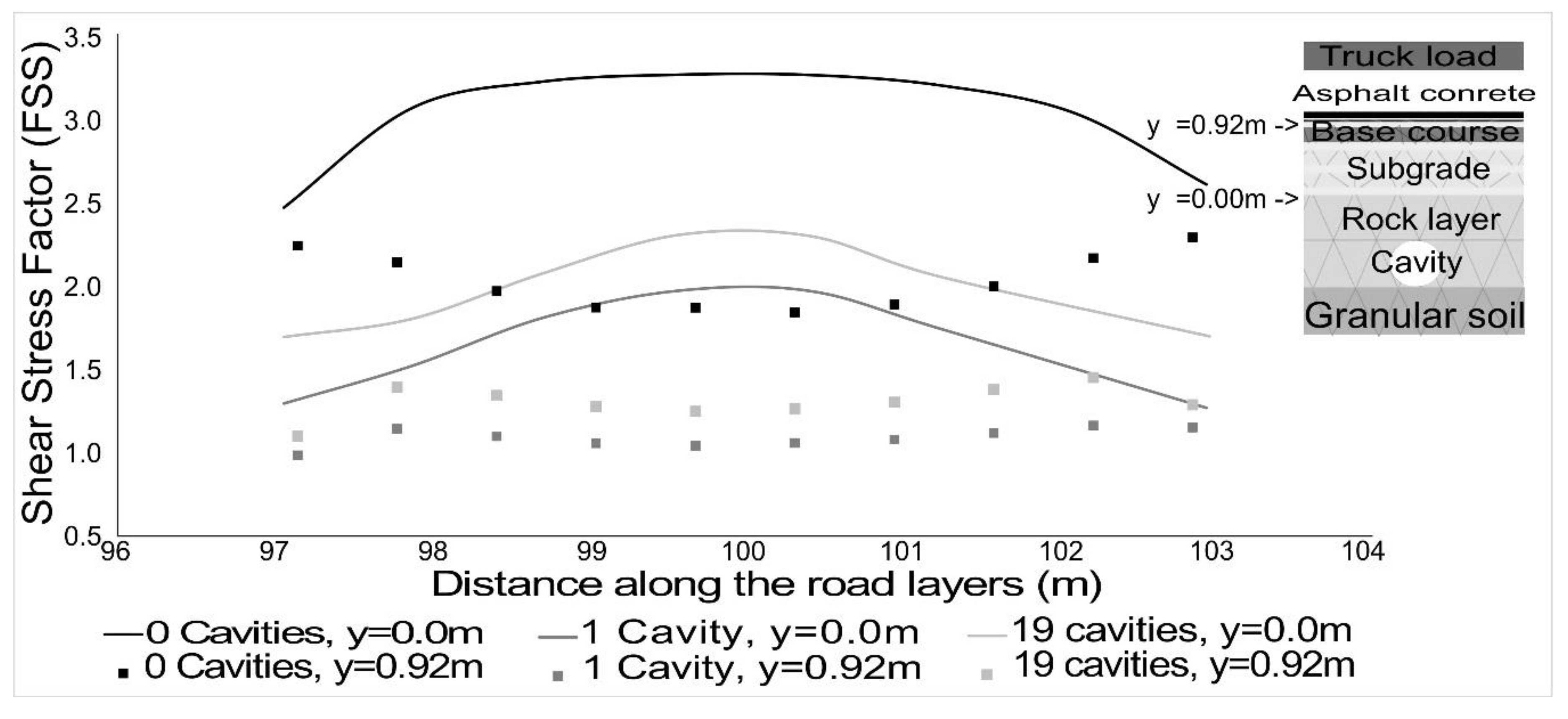
Figure 7 shows the
FSS along of two road layers at y = 0.0 m and y = 0.92 m in the road structure, considering only the truck load and the cavities without geogrids. Results as taken as a point of reference to have comparisons when the geogrids are added in the structure. In this analysis, the
Rinter# value between the road layers was
Rinter1 = 1. Good performance was observed in the structure with static load and 0 cavities, producing values greater than 2 of the Shear Stress Factor (
FSS) in the base of the structure (0 cavities, y = 0.0 m) and around of 2 in the top of the base course (0 cavities, y = 0.92 m). In the top of the structure road (y = 0.92 m) with 0 cavities, the
FSS is lower than in the base course layer, because it absorbs more of the static truck load stress and a lesser
FSS is developed in this layer.
This same Figure shows the performance of the road layers with the truck load and 1 and 19 cavities are simulated in the model. When there is 1 cavity in the central axis, the
FSS decreased in both levels, at the top of the base course layer (1 cavity, y = 0.92 m) and in the base of the structure (1 cavity, y = 0.0 m). After that, the
FSS has a slight increase in the road structure, pointing out that the
FSS value depends on the separation of the cavities with the road structure; furthermore, the failure of the cavities has reached its maximum deformation and the
FSS is practically 1. Relying on
Figure 7, the need to reinforce the structure due to the reduction in the FSS for cause of the cavities in the ground.
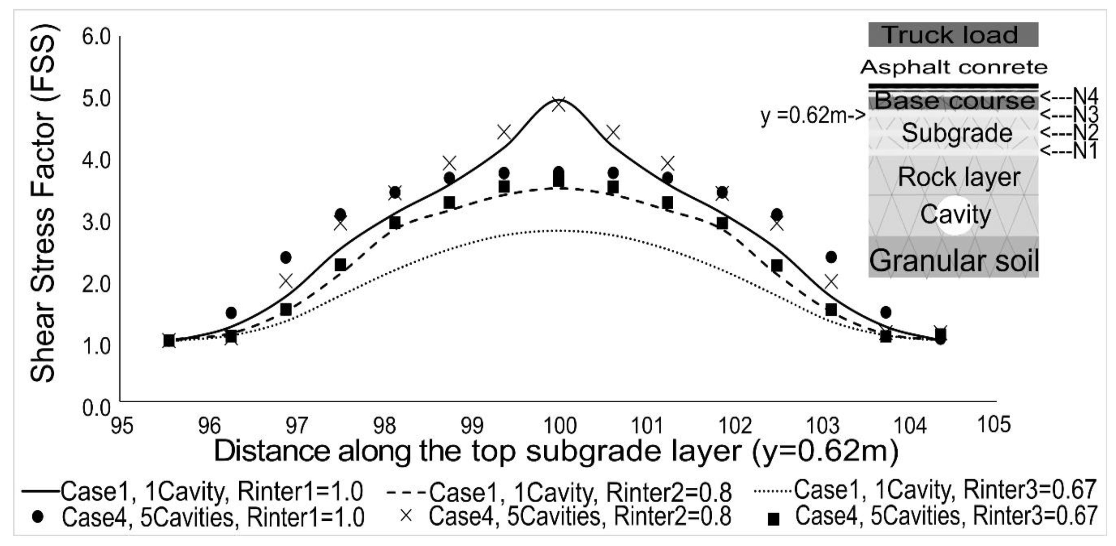
Influence of the three interface values
Rinter1 = 1,
Rinter2 = 0.8 and
Rinter3 = 0.67 are illustrated in
Figure 8 at y = 0.62 m, along of the top of the subgrade layer. Results for Case 1 (only one geogrid in the
N1 position) and Case 4 (four geogrids located in
N1,
N2,
N3,
N4 depths) show the influence of the 1 cavity and 5 cavities in the bedrock. The influence is in the reduction of the
FSS values when the interface value
Rinter# is decreased, which points out that Case 1, 1 Cavity,
Rinter3 = 0.67 and Case 4, 5 Cavities,
Rinter3 = 0.67 generates less
FSS in the top of the subgrade layer (y = 0.62 m) than the other interface values of
Rinter1 = 1.0 and
Rinter2 = 0.80. In the same way, it is possible to observe that when more cavities are developed the
FSS is increased, due to the failure of the cavities and in some way the stabilization of the surface terrain.
From this graph and for the next presented results, the interface Rinter3 = 0.67 that caused the most unfavorable Shear Stress Factor (FSS) was selected. Furthermore, when only a geogrid is considered in the road structure, the FSS can change markedly in the road centre.
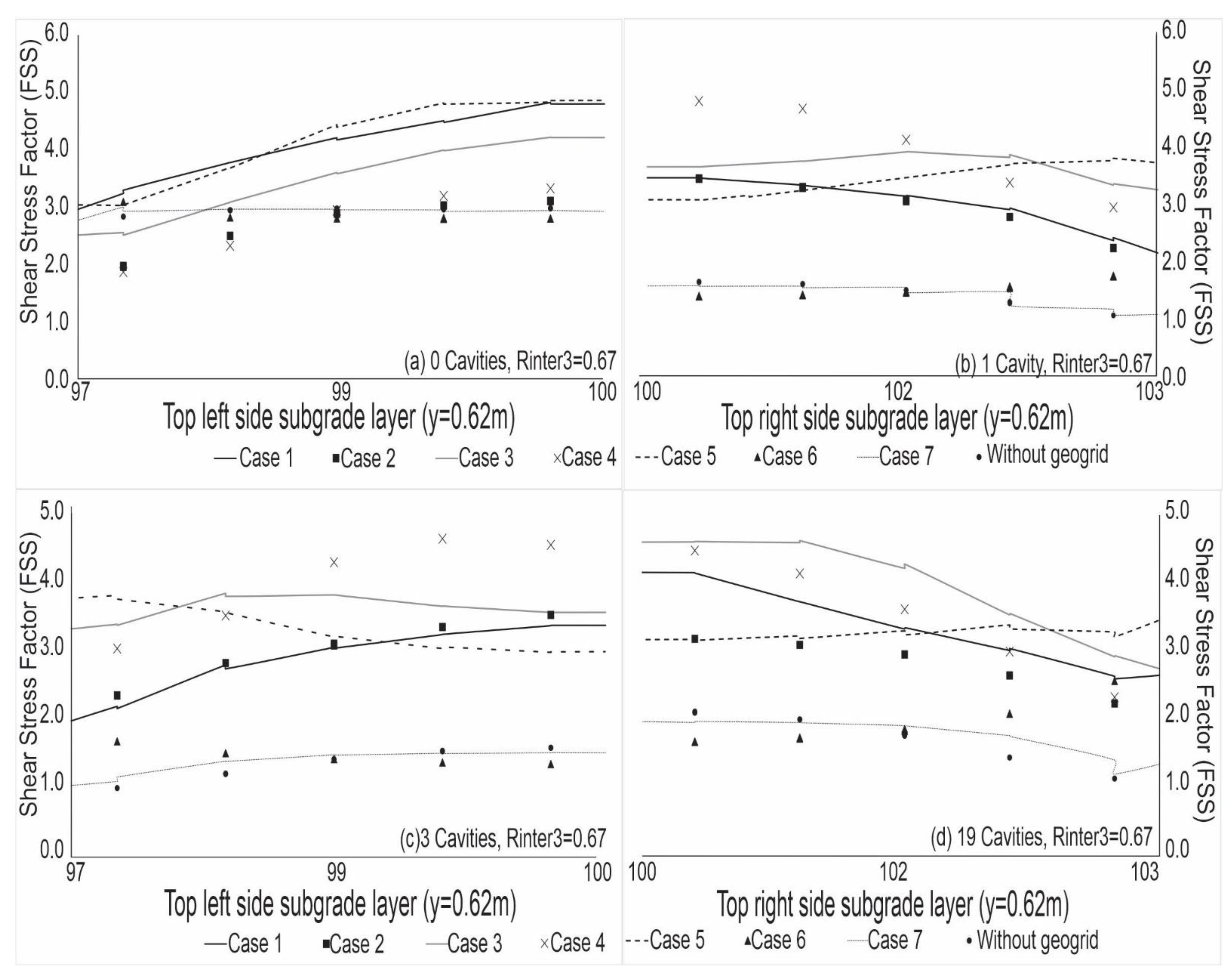
4.2. Mobilized FSS in the Different Road Layers for the Seven Analysed Cases
In
Figure 9 the impact in the
FSS is appreciated in the top of the subgrade layer (y = 0.62 m) for all the Cases and for a R
inter3 = 0.67, considering the truck load and 0, 1, 3 and 19 cavities. For
Figure 9a) with 0 cavities and the truck load, the Cases 1, 3 and 5 (black line, grey line and dashed line respectively), enhance the road structure increasing the
FSS compared to the Case without geogrids (black circle marks). When there is 1 cavity (
Figure 9b), the
FSS decrease in the top of the subgrade layer compared to the graph with 0 cavities and the Case 4 (cross mark with
N1,
N2,
N3 and
N4 geogrids) is the best combination to improve the structure reaching a maximum
FSS = 4.8 in the center of the road. Cases 1, 3 and 5 are slightly lower in its
FSS values. When there are 3 and 19 cavities in the model (
Figure 9c,d), Case 4 also has the higher
FSS, followed by the Cases 1, 3 and 5. In this Figure, the increase in the
FSS is associated to the soil stresses arrangement from the 3 cavities to the 19 cavities in the model, corroborating the results obtained in
Figure 8 but, for the seven cases using the improvement of the road structure with geogrids. Evidently there are some cases that the increment in the
FSS value is enhanced such as the Cases 1 and 3. On the other hand, Case 6 (geogrids in
N3 and
N4) and Case 7 (geogrid in
N4) indicate with the triangle marks and the dotted line respectively, show no improvement in the subgrade layer, concluding that the reinforcement in the base course layer is negligible for the subgrade.
The performance in the base course layer (y = 0.92 m) is presented in
Figure 10 with the same considerations as the previous Figure. In
Figure 10a) with only the truck load and 0 cavities, the Cases 1 and 6 have higher
FSS than the Case without geogrids and when there is 1 cavity (
Figure 10b) the behavior is divided in two groups, one with
FSS more than 2 and the other lesser than it. Cases 2, 3, 4 and 5 present the higher values and this behavior is the same when there are 3 cavities in the model. On the other hand, when there are 19 cavities (
Figure 10d) the behavior is similar with the particularity that the Cases 1 and 6 increment their
FSS values. For the top of the base course layer (y = 0.92 m), only Case 7 (one geogrid
N4, y = 0.92 m) does not show an improvement in the
FSS.
According to the
Figure 9 and
Figure 10, Case 3 and Case 5 (grey lines and dashed lines respectively) are the best combinations to increment the
FSS in both, the subgrade and the base course layers. Case 2 is also an adequate combination since its
FSS value does not vary a lot with the different numbers of the cavities, and despite that in the subgrade layer it does not have a higher
FSS, this combination improves the base course layer. Highlighting that in order to generate higher
FSS in the road layer, the best option is to enhance the middle and the top of the subgrade layer. Case 4 (cross marks) does not represent an adequate option due to the excess of geogrid additions which results in the cost of the road.
4.3. Stress Paths (τmob − p’) and Kinematics in the Different Road Layers Using Geogrid Additions
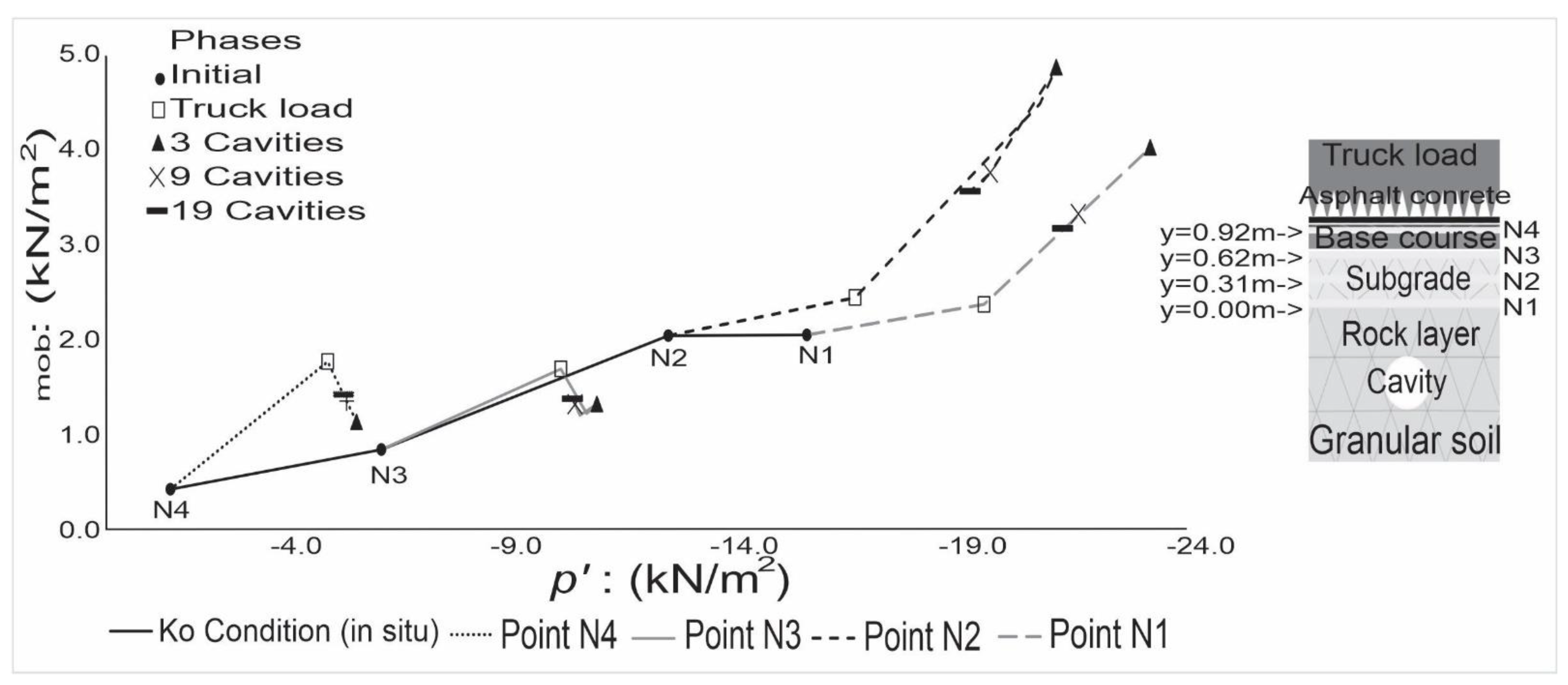
Figure 11 illustrates the stress paths (τ
mob −
p’) along of the road structure for Case 3 with a
Rinter3 = 0.67. The graph begins with the
K0 condition (in-situ stress), taking y = 0.92 m depth,
N3 y = 0.62 m,
N2 y = 0.31 m and
N1 y = 0.0 m geogrids in its respective depths. In the graph the black continuous line represents the
K0 condition (in-situ). When the truck load is applied in the road surface (empty squares in the graph), the principal stress (
σ’
1 =
σv) is increased in all the road structure layers behaving as a triaxial compression test. When there are 3 cavities in the soil (black triangle in the graph), the stresses change their direction in the first two depths (y = 0.92 m and
N3, y = 0.62 m), particularly the shear stress decrease with a slight change in the
p’, which means that the
σ’
3 =
σh increase presenting a passive pressure. At 0.31 m (
N2) and 0.0 m (
N1) positions, the
τmob stresses are increased with the
p’ stresses, reaching their maximum values when three cavities are developed in the ground (compression behavior). In the model with more of 3 cavities the stress changes, reducing having a passive pressure behavior.
Furthermore, this Figure illustrates that the stresses are superior in the subgrade of the road structure, verifying that the subgrade layer is the most unfavorable layer in the road structure. The behavior of the stress paths in the Case 3 is the same for all the Cases (
Table 2) and for the structure without geogrids, with the difference in the numerical values.
Figure 12 shows the mobilized shear stress (
τmob) evolution in the road structure for the Case 3 (
N1, y = 0.0 m),
N2, y = 0.31 m and
N3, y = 0.62 m), underlining that the base course layer gets more stressed than the subgrade layer due to the truck load. Nevertheless, the first cavity (
Figure 12c) causes a tension between
N1 and
N2 levels in the middle of the road structure. This tension is dissipated as there are more cavities in the granular soil (
Figure 12d). These kinematics confirm that the subgrade layer is the most stressed place of the road (
N1 and
N2 depths) and that the stresses in the layers vary depending on the number of cavities in the model.
4.4. Stress Paths (τmob − p’) in the Rock Layer Analyzed with Geogrids in the Road Structure
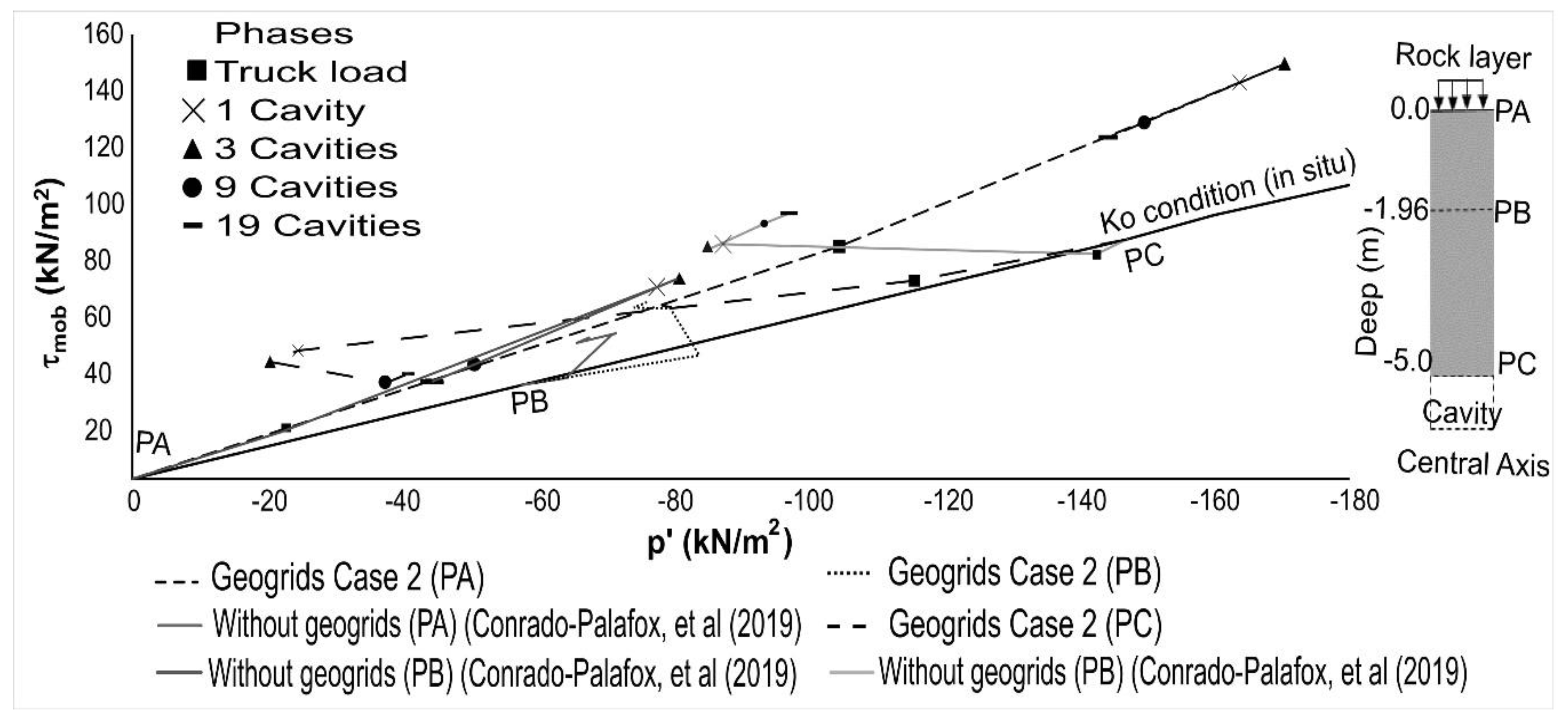
The
τmob −
p’ stress paths in the rock layer are presented in
Figure 13 in three different depths y = 0.0 m, −1.9 m and −5.0 m and considering these when there are geogrids (long dashed lines) and without geogrids (grey lines). This last stress paths were collected from the article [
3]. It is important to point out, that the magnitude of the static load, is the same in both papers. Nevertheless, in this paper the structure of the road was modelled and the truck load was applied over the asphalt layer and in the first work only one total load (truck load and road structure) was considering directly in the rock surface.
Furthermore, the results shown with geogrids correspond to Case 2 and with the road structure contemplated in the numerical model. Case 2 was chosen in function of the results presented in the Mobilized FSS in the different road layers for the seven analyzed Cases section, remembering that the best behavior Cases were Case 2 and Case 3 in its performance.
In the surface rock layer (PA, y = 0.0 m), the stresses are increased until the 3 cavities (black triangle mark) in both cases (compression behavior). When subsequent cavities are developed, the stresses return following the same line and due to the relaxation effect of the horizontal stress (σ’3 = σh) with the particularity that in the model with geogrids (N1 and N2 positions—Case 2) it generates stresses with higher values due to the differences in the numerical modeling.
For the two results (with in without geogrids), in the −1.9 m depth (PB), the inflexion point is between the 3 cavities and the truck load (square marks), where the τmob increases reaching the maximum value with 19 cavities (black block marks), that means that an effect of the active pressure is presented rock material tends to be get into the holes developed in the ground.
At the base of the rock layer (PC) with geogrids in N1 and N2 positions, the behavior changes in respect to the previous depths. The p’ decreases until the phase with 3 cavities in order to change its direction (excavation effect) and the reduction of the τmob when there are more cavities, opposite to the condition when there are not geogrids. This means that the effect of the geogrids benefits the ground behavior when the mobilized shear stress is lesser.
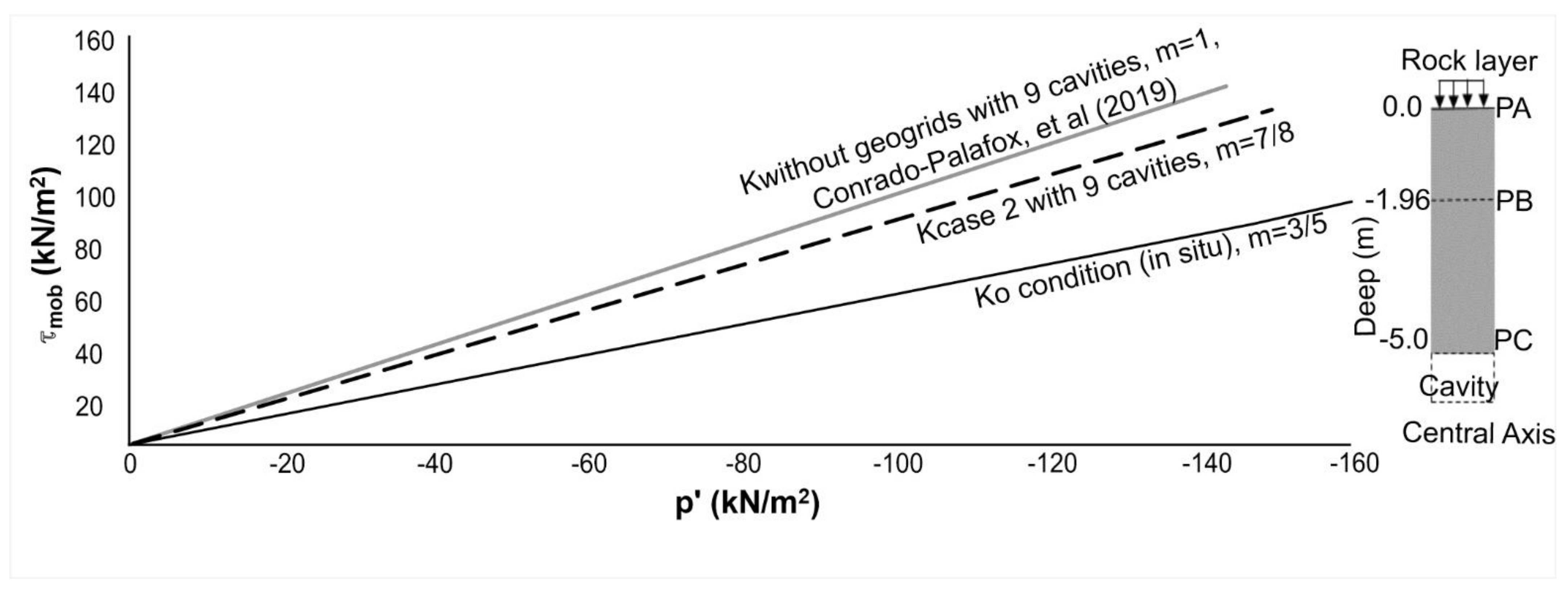
To conclude this section and following the stress paths behavior described in
Figure 13, a trend line was proposed and was named as
Kcase2 and is presented in
Figure 13. This line was obtained by joining the
τmob − p’ points in the phase with 9 cavities at the different depths of the rock layer and when the road structure has 2 geogrids in
N1 y = 0.0 m and
N2 y = 0.31 m depths (Case 2).
This trend was compared with the
Kwithout geogrids line proposed by Conrado-Palafox [
3], where its results indicated that the stratigraphy without cavities supports the highway load; nevertheless, with 9 cavities in the granular soil the stress path changes direction, affecting the terrain surface and presenting a subsidence.
Kcase2 trend indicates that with geogrids in the road structure, the τmob are lesser in the rock layer, resulting in a minor slope. This tendency corroborates the satisfactory influence of the inclusion of the geogrids in the amelioration of the road structure when exist cavities in the ground. (
Figure 14).
5. Discussion
The present study was designed to determine the effect of the geogrid layers in a road, affected by the subsidence created by the cavities in the subsoil. Results are shown in terms of the stress paths, due to the stresses permit to visualize, which of the three layers of the road (subgrades and basecourse), was less compromised in the moment of the subsidence developed in the terrain. Combination of the geogrid positions were simulated to find the best combination.
The findings obtained based on these finite element modeling, confirm the increase of stresses and the low values of stress shear factor when there are many cavities in the model, but also confirm the stabilization of the terrain after several open cavities, because the stress shear factor in the road layers increase. This performance is attributed to the position of the cavities, those closest to the road affect more.
As it was expected, the combination Case 4 of geogrids is the best combination to improve the structure. However, this reinforcement is unacceptable in the construction community due to the cost to build roads with geogrids. Furthermore, this study points out the unnecessary to reinforce the base course layer, because the damage is absorbed mainly in the subgrade layers. This conclusion must be analyzed under cyclic loads on the crest of the road, which certainly would affect the base course performance.
This study set out the necessity, to reinforce the subgrade layer and most importantly only reinforce the middle and the top of the subgrade layer to reduce the stress shear factor in the road structure due to the cavities. Furthermore, the decrease in the slope of the stress paths (τmob vs. p’) in the rock layer with the presence of the geogrids in the road was founded in this study, which guarantees a better behavior.
In general, previous studies have pointed out the geogrids as an adequate reinforcement method, for several structure problems such as poor bearing capacity in the road layers, clay problems in the subsoil and problems due to one cavity under the road. With this study it is possible to verify the geogrids, as a solution in terrains affected by karsticity, specially with several cavities in one area.
Further studies, which take these results into account, will need to be undertaken to increase the improvement of the geogrids in the road construction. As well as future investigations based in real road construction in similar karst terrain are recommendable to join the analytic results with construction performance and in the future modify the Mexican road construction in karst terrain standards and considering the effect of cyclic loads.
6. Conclusions and Future Research
The infrastructure construction is necessary in the world and this will continue even in karstic terrains. The high frequency of mechanical failure in karst terrains is a handicap due to the dissolution of the young limestone. Therefore, substantial improvements in the prevalent construction practices are needed, due to the demographic and economic evolution.
In this work numerical FEM models are presented for a typical road structure, to verify the effect of the reinforcement provided using geogrids, when cavities in the ground are presented and developed over time. To select the optimal numerical model, the granular soil and the bedrock was modeled using parameters found in the endemic geomaterial in Merida, Mexico. The dimensions and the thickness layers of the subgrade, the base course, and the asphalt concrete, correspond to those used in the typical constructions found in the zone as well as its materials characteristics. Geogrid characteristics simulated are for an elastic material and the values of its resistance were obtained of the literature references regarding this topic.
Several interfaces Rinter values were studied to study the influence of the adherence among the road layer and the geogrids. Results illustrate that a decrease of the FSS value is obtained in the road layers with the decrease of the interface value.
In this work, the nine cavities in the granular soil of the stress path have unfavorable behavior, because they presented a change in the stress path direction, affecting the terrain surface and presenting a subsidence, despite cavities existing away from the road structure. These results are corroborated with the FSS that stop to decrease and since shear stress is dissipated. According to the stress paths presented and the kinematics, the subgrade is the most stressed layer in the structure when the cavities are presented in the numerical model.
The FSS of the road with 2 or 3 geogrid layers (Case 2 and Case 3) showed the best improvement when cavities are present in the subsoil, concluding that the geogrid enhances the stress distribution and generates less τmob in all structural road layers, nevertheless the subsidence will continue to be present on the surface of the rock layer but with a minor displacement.
From the numerically generated stress paths when geogrids are added, a trend line was proposed following the
τmob presented in the ground. This line unites the most unfavorable phase that is presented with 9 cavities in rock layer and when the road structure has 2 geogrids in the road structure. This trend was compared with the line that did not use geogrids proposed by Conrado-Palafox [
3], which represents the buffering of the stresses when geogrids are used.
Finally, it should be noted, that additional studies are needed in order to improve the computational karstic model for example incorporating the cavities in a random location in the subsoil and to evaluate the geogrid in the base course layer position under cyclic load considering the karsticity. This study represents a benefit for the regions with karstic soils by proposing a change in the construction practices.


 ,
, 


