Bridge Inspection and Defect Recognition with Using Impact Echo Data, Probability, and Naive Bayes Classifiers

Abstract

Interpretation of IE data have been carried out by analyzing IE signals in frequency domain to determine the maximum frequency. However, the current peak frequency method can be inaccurate. The purpose of this research is to introduce features in IE signals that can be used for effective classification and interpretation for bridge deck evaluation through statistical analysis and Naive Bayes classifiers. The dataset contained IE data collected from eight slabs created at Advanced Sensing Technology FAST NDE laboratory (FHWA). A set of statistical features in time domain, normalized peak values, and length of preprocessed signals were used to classify the IE data, statistically. Then, Naive Bayes classifiers was employed to recognize defect area. Finally, the result of statistical classification was compared with frequency approach. The result shows that 19 and 21% of the IE signals collected from the defect area have multiple peaks, respectively. However, 85% of the IE signals collected from the sound set had only one peak. A probability classifier was used to find the relationship between the result of the frequency method and statistical analysis. The result shows that 10% of the IE signals were usable for estimating the thickness in the sound group.

1. Introduction

Impact Echo (IE) test is a point-wise evaluation method that is used to record a structure’s response at different locations for multiple proposes [1]. For example, IE data can be used to indicate the thickness of a concrete slab [2] crack localization [3], detection of subsurface flaws such as delamination, honeycombing [4,5], deboning [6], and voids [7] in different experimental set ups. Raw IE data are signals where the horizontal axis represents surface acceleration of echo waves due to an impact at a point of structure and vertical axis represents time of wave travel in the structure. Therefore, using IE data without interpreting them could be difficult. There are different ways to interpret IE data. The most common method is called peak frequency method where Fourier Transformation is applied on IE signal determine backwall frequencies or the ones associated with defects. Several researchers have been working on pattern recognition of the frequency spectra of IE signal for delamination detection. For example, Colla et al. (2003) evaluated the impact of source frequency on the quality of impact echo data. The result of this research showed that the maximum energy with expected measured frequency should be considered to reach the maximum quality of impact echo data. The location of the impact echo source and boundary condition could be influenced by the signal patterns, reflecting the difficulty of interpreting IE data via using the frequency approach [8]. Nguyen et al. (2017) indicated the IE signals with two distinguished peaks or IE signals with one peak occurring at the higher or lower frequency response of flexural mode could suggest the presence of a defect in concrete [9]. Yeh et al. (2018) employed a phase spectrum approach to distinguish cracks and the location of reinforcing bars [10]. The result of some studies revealed that the shape of IE signals, in terms of frequency responses, does not always follow the theoretical description to show defect area [11]. Moreover, the boundary condition of structure could influence the frequency and shape of signals as the waves reflected from lateral boundaries can significantly affect the time-domain signals and spectra [12]. Therefore, analysis of IE data using the time-domain features can be considered as an alternative to the peak frequency method. Researchers have looked into extracting statistical features of IE for more classification to measure concrete thickness [13] and to generate Probability of Detection [14]. Using Bayesian classification method and machine learning, IE signals were classified with 92.3 accuracy (Pagnotta et al., 2018) [15]. Rashidi et al. (2020), used probability distributions and the square root of the Jensen-Shannon divergence to evaluate the Haymarket Bridge deck (located in Virginia, U.S.) [16]. The results of the research showed that the use of a probabilistic method can lead to comprehensive statistical features and consequently to a tool for IE data interpretation.

The authors hypothesize that the value and the location of extremums in IE signals can be used to extract different features for robust delamination detection in concrete bridge decks. These features can be used to train machine learning classifiers trained directly on IE signals. Machine learning has been considered a common numerical approach for the detection of defect areas [17], for thickness measurement [18], and rebar areas of the reinforced concrete beam [19] using IE. In the majority of machine learning algorithms, user input is required to select the features considered for classification. Recently, Dorafshan et al. (2020) developed a deep learning model for training convolutional neural networks to detect artificial delamination in laboratory-made reinforced concrete specimens where the features were extracted autonomously and through training [11,20]. The training datasets of the convolutional neural network (CNN) in raw IE data collected from the subsurface of structure with no pre-processing. Although deep learning has many benefits toward conventional machine learning models, they require large annotated datasets to be accurate, which are rare. Therefore, further development of more robust deep learning models could be challenging, limiting researchers to classical machine learning algorithms.

The purpose of this investigation is to provide a better understanding of IE signals that can be incorporated with unsupervised deep learning models for bridge deck evaluation.

Zheng et al. (2018) used a pretraining process to reduce the overfitting of image classification [21] to improve the performance of their proposed CNN. Training CNN to learn features and recognize faults in data was applied to solve a multiclass problem [22]. The result showed that the connection between features, which were trained by CNN, and the accuracy of classification are higher than conventional training approach [22]. However, none of this information is dedicated to interpret impact echo data.

Against this backdrop, this study aims to detect defects and sound zones by combining time-domain features of IE data, frequency analysis, Naive Bayes classifiers, and probability density functions. For this purpose, the IE peak values, the corresponding time range, and the normalized peak values of several laboratory-produced samples were extracted. A mathematical algorithm was developed to filter IE data to extract distinguishable peak points. Second, a statistical approach and probability density function (PDF) were used to obtain statistical properties of the IE data on defective and healthy areas. Third, this statistical information was used to classify the dataset (defect or sound) before using the Naive Bayes classifiers to create a pattern for predicting the sound and defect locations. Finally, the new training datasets were prepared for Naive Bayes classifier models. The scope of the research is as follows:

• Developing a preprocessing approach based on distinguishable peak points;
• Using probabilistic methods to find a relative pattern for detecting defects or sound regions based on the features of the IE signals;
• Using probabilistic methods to find atypical IE data or data that does not follow the general pattern of IE signals in each dataset. Classification of the IE data in terms of defect or sound based on the feature of preprocessed IE signals.

2. Method

2.1. Description of Data

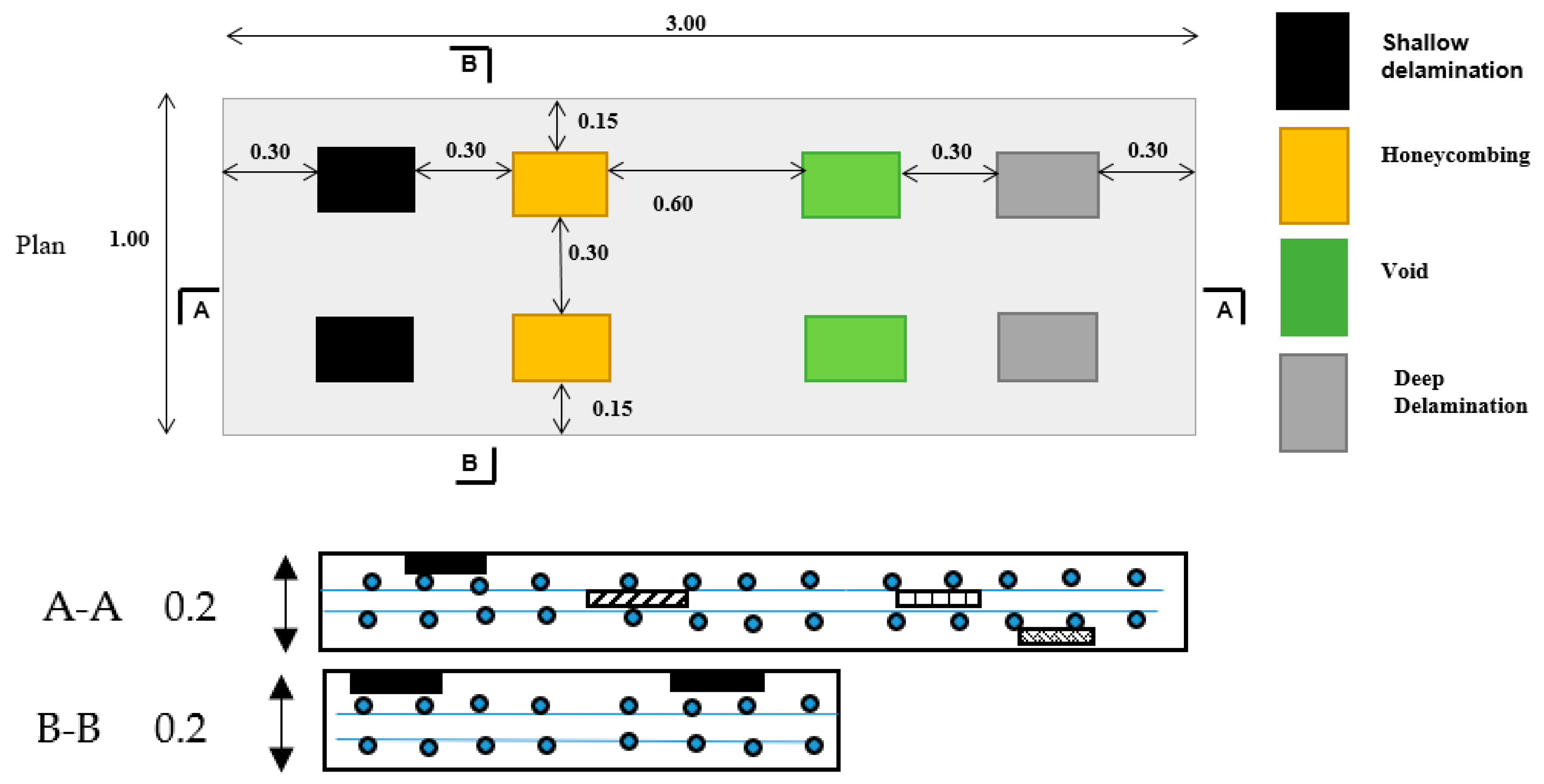
In this research, the dataset contained IE signals collected from eight slabs with artificial defect created at Advanced Sensing Technology FAST NDE laboratory) (FHWA) [11]. The length, width, and thickness of the slabs were 3.0, 1.0, and 0.2 m, respectively. All slabs contained four types of artificial defects including shallow delamination, deep delamination, honeycombing, and voids. The height of the defect was 0.3 m while its width was 0.2 m. Figure 1 shows the defect type and the plane of the slabs. More information regarding to the type of defects, concrete age, and material can be found in [11].

2.2. IE Method

IE device used for data collection contained a mechanical spherical impactor with a diameter of 3 to 12 mm to generate wave, and a displacement transducer located roughly 5 cm near the impact dot [11]. The produced wave propagates through the surface of structure and reflected at interface to find discontinuities area like defect. A sensor was put near the impact to record the echoes. The output of the IE device can be looked at in two formats: waveform and spectrum. Spectrum can be obtained through applying Fourier transform to generate frequency response of the IE data. The thickness of the slab was obtain by Equation (2).

$$t=\frac{\beta *{\complement }_p}{2f_h}$$

(1)

where$({\complement }_p)$,$\left(f_h\right),$ (t), and $\left(\beta \right)$ are impact echo’s velocity in meter per second (m/s), associated frequency, thickness of the concrete in meter, and shape correction factor, respectively.

2.3. Description of the Proposed Method

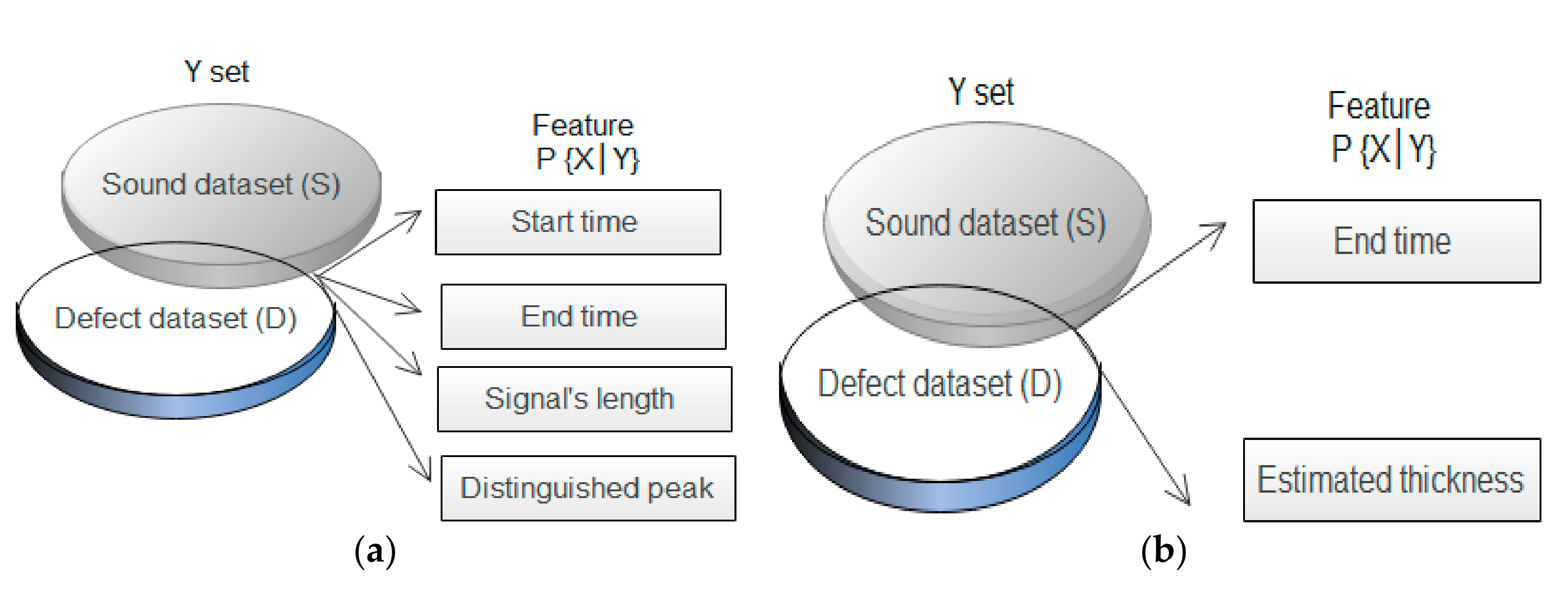
In this research, the features of IE signals like time and frequency domain of distinguished peaks in the IE signals, normalized peak value, length of the IE signals contained peak values was considered to classify IE data. Figure 2 shows the Naive Bayes classifiers constructed using a set of proposed features in the time domain of IE signal. Probability density functions and Naive Bayes classifiers were used to interpret and classify preprocessed IE signals. Therefore, the method of the present study comprises two main parts, which are described, here:

• The use of preprocessing filtering approach to detect distinguished peaks, which leads to statistical classification and detection of IE signals. The preprocessed IE signals were generated based on distinguished peaks in IE signals as seen Figure 3. Generally, the frequency domain corresponding to the peak point of IE signal has been employed to evaluate the behavior of IE signals in the frequency approach. However, some research in computer science shows the peak values of signals can be used to classify data in time domain [23]. To evaluate IE signals in time domain, detection peak algorithm was employed to cut signals based on distinguished points. To do this, as shown in Figure 3, any point with values less than 10% of the absolute maximum value was removed from the start and end of the IE signal. This will not have a major impact on the analysis, since peaks with values smaller than 10% of the absolute max will not change the frequency repose significantly. This claim was validated through applying the proposed preprocessing filtering approach on a set of random IE signals, which showed the frequency response of raw and processed signal impact echo signals were the same when the trivial points were removed. Finally, the IE signal was divided into five segments. Time domain (starts and end point), normalized peak values $\left(\frac{local peak values }{absulate maximum value }\right),$ and length of preprocessed IE signals was obtained for each segment as the futures of IE signals.
• Probability and Naive Bayes classifiers were used to classify data. In the following, the statistical and Probabilistic classification was discussed.

  -

  Statistical method

  The probability density function (PDF) can be used to see the probability of occurrence of samples, it also can be used to remove outliers or atypical data from an original dataset. Understanding the PDF for a group of data could be useful to determine data distribution type, mean, and variance, special patterns for classifying. A set of PDFs for IE data were generated based on the feature of IE signals. Easy Fit [24] was used to fit a series of known probability distribution to the IE PDFs. Additionally, 3-D representation of pdf (probability density function (f(x))) were built to identify correlation between the variables.

  -

  Probabilistic classification

  A probabilistic classifier is considered as a classification approach in machine learning, which is employed to estimate the probability that each data set occur with using input layers. Naive Bayes classifiers were employed for classification by applying Bayes’ theorem and independence assumptions between input layers [25]. In this research, the relationship between input variables such as signal peaks, length, end and start time of preprocessed signals, and the output layers (defect or sound area) was obtained. In addition, the relationship among the IE signal’s end time interval and the amount of the estimated thickness was evaluated. As seen in Figure 2, two models were generated as probabilistic classification models. For the first model, the input layer contained the length of signals, average of peak value, start and end time of preprocessed IE signals, and the output layers are defect and sound set. For the second, in the input layer is contained the estimated thickness, which was obtained using frequency approach and end time of preprocessed signals.

Figure 3 shows the methods and main step of this research.

3. Results

Frequency response of impact echo were employed widely to detect defect area. In this approach, frequency domain and distinguished peak point of IE signals were used to classify IE signals in three classes: good, fair, and poor [26]. The IE signals, which have a distinguished peak within the thickness resonance, were classified as good. In Fair condition, the principal concentration of energy was occurred in the thickness resonance band; however, a small part of the energy will be in the lower band of frequency. For poor or seriously deteriorated condition, higher frequency concentration can be seen in the lower thickness resonance band [26]. In this study, the authors propose combining the peak frequency method with features extracted from IE signals for precise classification.

-

First, the futures of IE signals in defected and sound regions were compared

-

The relationship between the estimated thickness, which was obtained by the frequency domain of IE signals, was compared to the features of signals in the time domain.

3.1. Statistical Result

-

Data classification based on the length of the signals

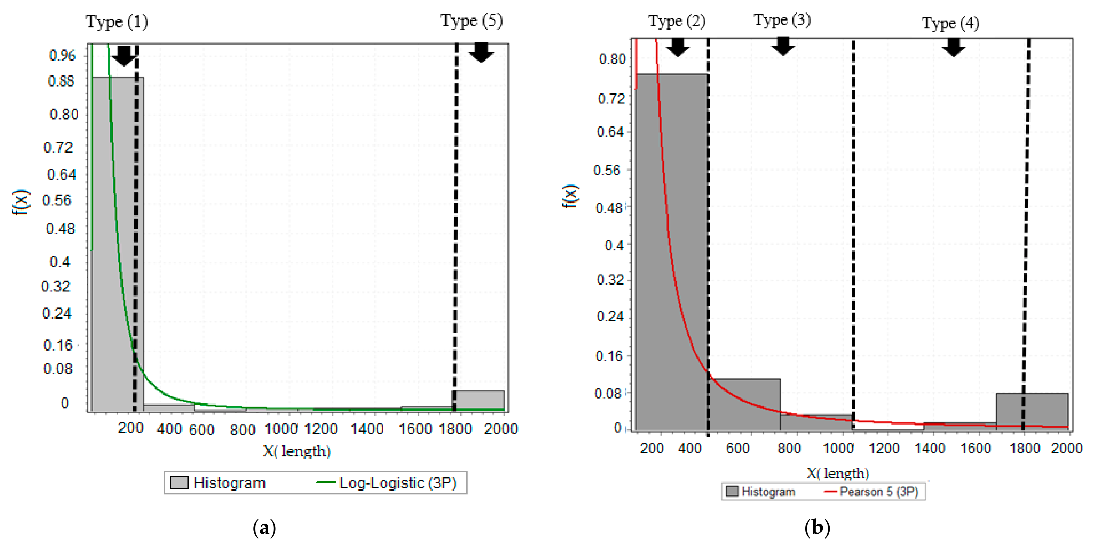
The lengths of all preprocessed IE signals for two groups of data (defect and sound) were used to construct PDFs and their best fit distribution. Figure 4a,b show the length dispersion of IE data for slab 2 defected and sound, respectively. After analyzing the length PDF graphs, it was made apparent that the IE can be classified into five types:

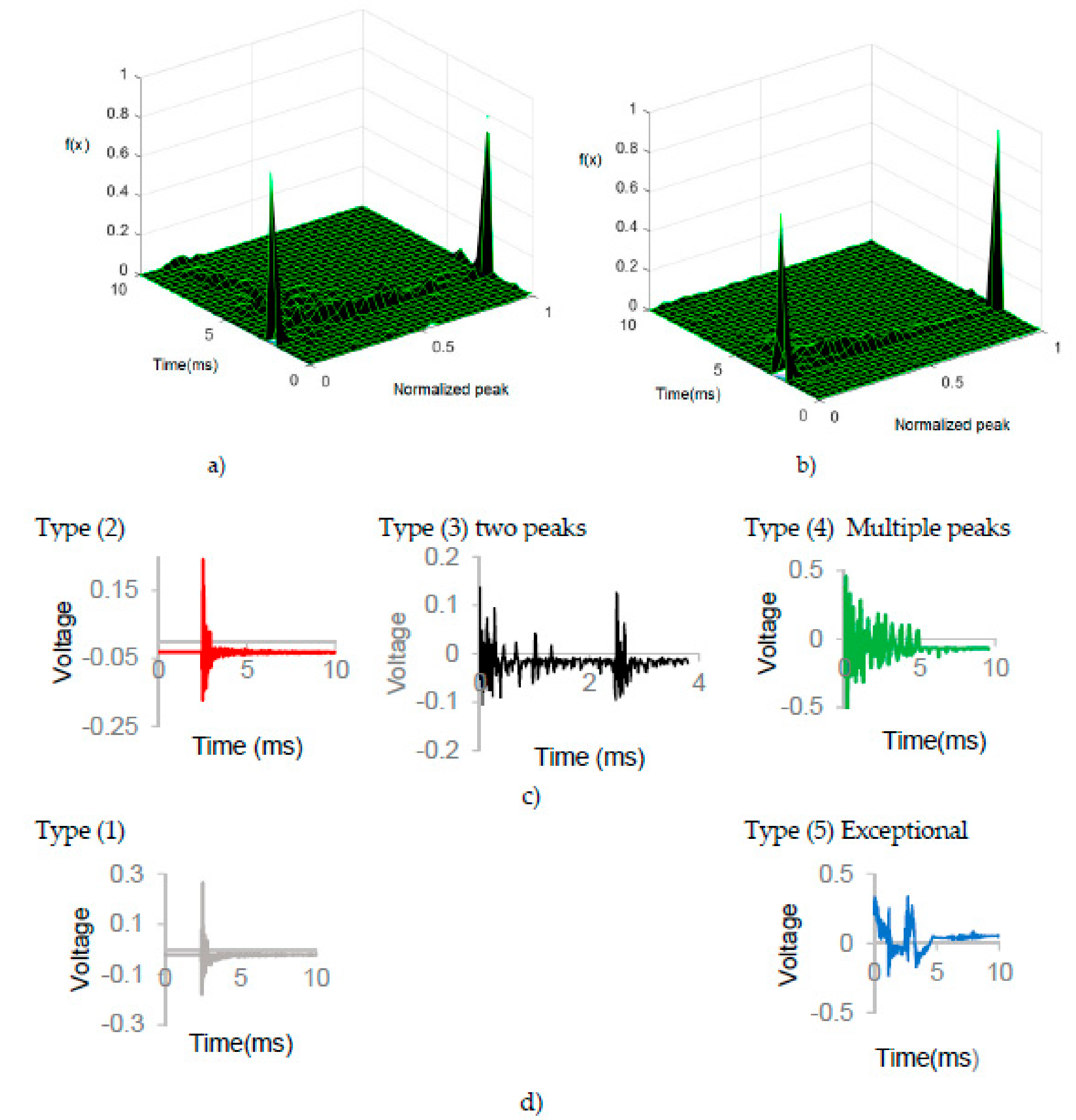
• Type (1), IE signals in sound group concluded one distinguished peak point with signal’s length contained 200 points or less.
• Type (2), IE signals in defect group concluded one or two distinguished peak points with the signal’s length contained 400 points or less than 400 points.
• Type (3), IE signals concluded one or two distinguished peaks in different times, the length of signals contained more than 400 points, and less than 1000 points.
• Type (4), IE signals concluded multiple distinguished peak points in different time intervals, the length of IE signals contained more than 1000 points, and less than 1800 points.
• Type (5), Exceptional IE signals, this type of signal broke the common pattern that was obtained by frequency analyses for classification in previous research. For example, some IE signals in the sound set were not cut by the proposed processing method due to their unusual shape.

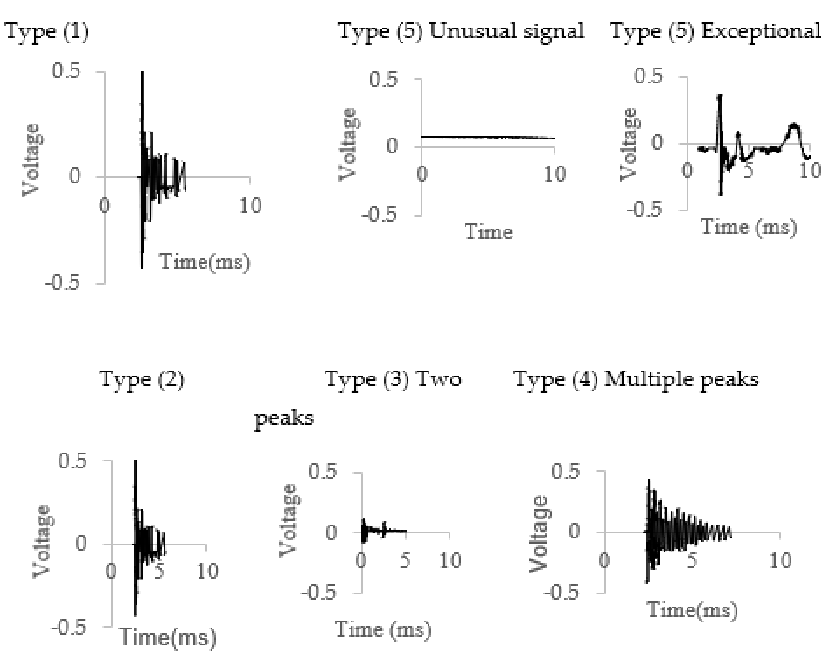
As seen in Figure 4b, type (2), (3), and (4) were normally observed in IE data collected from defected areas. In contrast, as shown in Figure 4a, most IE data extracted from sound regions were cut and classified into type (1) and (5). Figure 5 shows the examples of IE signal in different types. The length of preprocessed IE signals showed to be a proper indicator for classification. The IE signals, which were categorized as type (2), (3), and (4), could be used to detect defect zone. Since the proposed classes have overlap, the authors investigated time interval corresponding to normalized peaks. In general, the energy of IE signals collected from the sound zones were more concentrated in short interval time (type (1)). Therefore, the length of preprocessed signals in sound zones was shorter than IE signals collected from the defect area. Some IE data from defect or sound did not follow this pattern. Thus, the time or frequency domain for normalized peak value and length of signals showed to be the good indicator (only one peak (type (1) and (2)). The results of the PDF analysis of IE data are summarized in

Table 1. Probability result for preprocessed IE signals based on signal length for defect area.

Parameters	Slab 1	Slab 2	Slab 3	Slab 4	Slab 5	Slab 6	Slab 7	Slab 8	Mean
Number of data	64	64	64	64	64	64	64	64	64
Mean value	243.9	361.23	272.53	215.47	330.8	837.5	589	402	399
Coef. of Variance	1.39	1.39	1.04	1.22	1.23	0.96	1.2	1.13	1.19
Percentile 10%	104.3	100.5	94.50	90	98	114.5	111	111.50	103.14
Percentile 25%	114.75	110.75	105	114.50	119.5	130.5	123	129.75	118.41
Percentile 50%	134	132	160	145	151.5	358.5	187	189.50	180.38
Percentile 75%	197	334.75	289.75	168.50	306.7	1893	436	438.25	497.21
Percentile 90%	464.4	1108	664.50	399	1026	1984	1638	1238	1062.1
Best probabilistic fit	Gen- Extreme value	Pearson 3P	Log-logistic	wake by	Frechet 3P	Johnson SB	Pearson 3P	Burr	-----
f(x) for 0–380 points	0.86	0.76	0.82	0.88	0.80	0.52	0.72	0.70	0.755
f(x) for 380–900 points	0.12	0.09	0.16	0.10	0.09	0.11	0.14	0.18	0.122
f(x) for 900–1600 point	0	0.06	0.02	0.01	0.08	0.04	0.04	0.08	0.043
f(x) for 1600–2000 point	0.01	0.07	0	0.005	0.03	0.01	0.09	0.02	0.030
f(x) for unusual type	0.01	0.02	0	0.005	0	0.32	0.01	0.02	0.043

and

Table 2. Probability result for preprocessed IE signals based on signal length for sound area.

Parameters	Slab 1	Slab 2	Slab 3	Slab 4	Slab 5	Slab 6	Slab 7	Slab 8	Mean
Number of data	188	188	188	188	188	188	188	188	188
Mean value	262.53	302.95	155.74	127.83	262.53	227	245.31	122	216.5
Coef. of Variance	1.71	1.65	1.51	1.10	1	1.42	1.31	1.36	1.386
Percentile 10%	96	97	90.9	77.80	96	102	100.9	99.99	95.17
Percentile 25% Q1	107.25	104	99	95	108.25	113	112.2	109.25	106.2
Percentile 50%	126	119.5	114.5	110	123	129	133	122.5	122.1
Percentile 75% Q3	151.75	153.25	137.75	126.50	147	169	200	149	153.9
Percentile 90%	279.5	1359.5	157.70	149.50	446	402	501	210.40	441.2
Best probabilistic fit	Log-logistic	Burr 4P	wake by	wake by	Cauchy	Levy 2P	Burr 4P	Burr 4P	----
f(x) for 0–250 points	0.9	0.87	0.98	0.98	0.88	0.88	0.86	0.94	0.911
f(x) for 250–900 points	0.05	0.04	0.01	0.01	0.05	0.08	0.10	0.02	0.042
f(x) for 900–2000 point	0.02	0.03	0.002	0.005	0.06	0.03	0.02	0.02	0.024
f(x) for unusual (type 6)	0.02	0.05	0.008	0.005	0.01	0.01	0.01	0.01	0.020

, for defected and sound IE data, respectively. According to the result, roughly 90% of the preprocessed IE signals from the sound zones concluded 210 points, and these signals have not distinguished peaks in different time intervals. The energy of signals was more concentrated in special and short time range without shifting to other bands. For defected concrete, the length of only 25% of short IE signals was concluded 400 points with two or multiple peak points. In this research, the probability density function (f(x)) and histogram was used to classify IE data. The goodness of fit was obtained among forty common fits and it is mentioned for each slab, and the result shows that the statistical fit distribution cannot precisely predict all the observed data. However, it could be used to estimate the distribution of most preprocessed IE signals.

The best fitted distribution and statistical parameters for the length of all processed signals were extracted from the PDF plots and summarized in Table 1 and Table 2. According to the result, roughly 90% of the preprocessed IE signals from the sound zones concluded less than 411 points and these signals have not distinguished peaks in different time intervals. The energy of signals was more concentrated in special and short time range without shifting to other bands. The length of 90% of preprocessed IE signals was concluded less than 1062 points in the defect dataset, which showed that the energy of signals was not concentrated in a small interval time, also 25% of IE signals have two or multiple peak points in different time intervals.

-

Data classification and statistical pattern recognition based on time interval and normalized peak values.

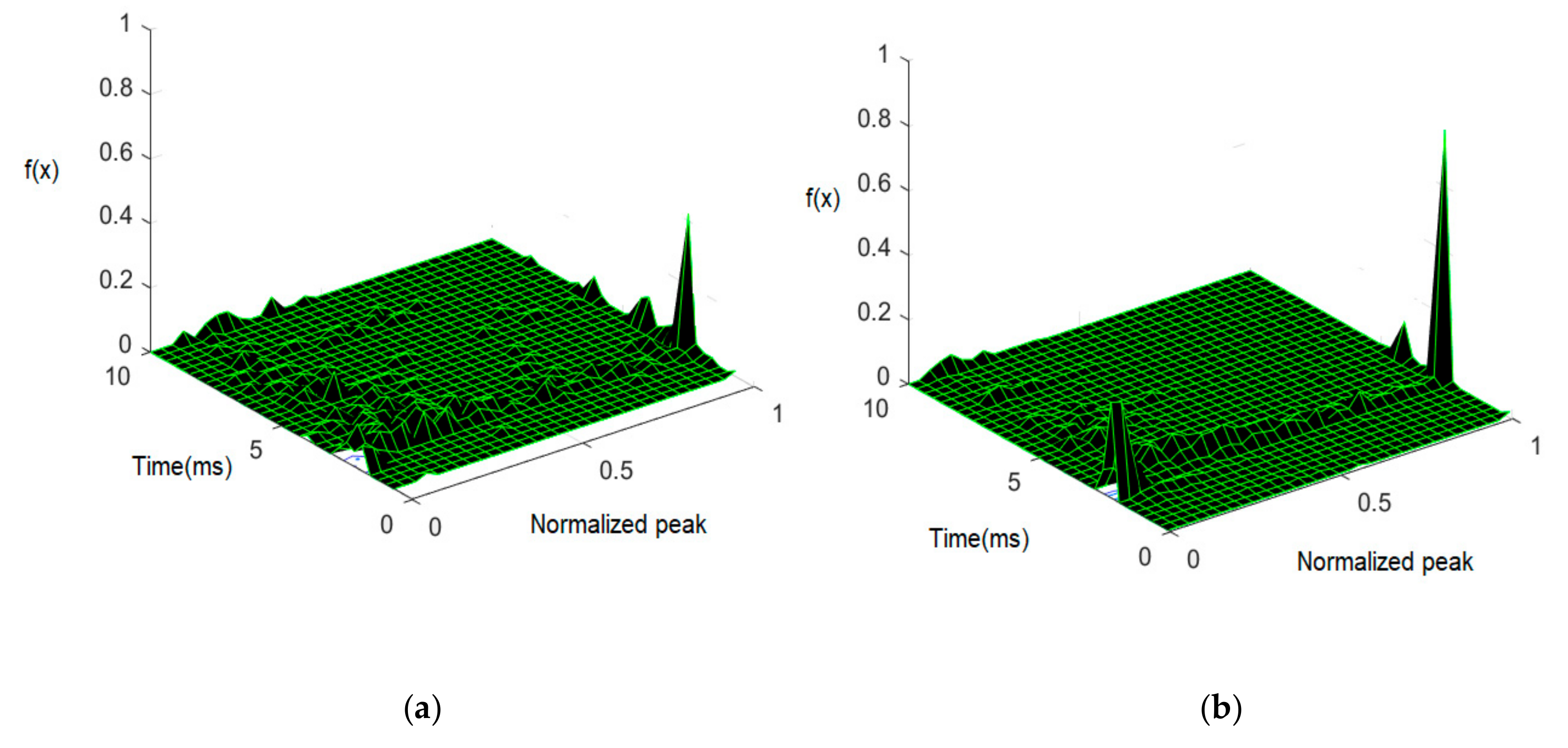
To increase the robustness of classification in this investigation, the values of absolute maximum and local peaks for all processed IE signals were obtained. Then, the local peaks were normalized with respect to the absolute maximum (see Figure 2).

Table 3. Statistical results based on time interval preprocessed IE signals collected from defect and sound part.

(a)
	Slab 1	Slab 2	Slab 3	Slab 4	Slab 5	Slab 6	Slab 7	Slab 8	Mean
Number of data 64 × (number of peaks for each signal = 5)	320	320	320	320	320	320	320	320	320
f(x) for number of peaks between 0 to 2 ms	0.05	0.02	0.67	0.22	0.13	0.25	0.07	0.09	0.21
f(x) for number of peaks between 2 to 4.5 ms	0.75	0.79	0.20	0.66	0.74	0.47	0.64	0.60	0.60
f(x) for number of peaks between 4.5 to 9.99 ms	0.20	0.19	0.13	0.12	0.11	0.28	0.13	0.31	0.19
(b)
	Slab 1	Slab 2	Slab 3	Slab 4	Slab 5	Slab 6	Slab 7	Slab 8	Mean
Number of data 188 × (number of peaks for each signal = 5)	940	940	940	940	940	940	940	940	940
f(x) for number of peaks between 0 to 2 ms	0.03	0.012	0.005	0.19	0.07	0.03	0.07	0.07	0.06
f(x) for number of peaks between 2 to 3.5 ms	0.88	0.90	0.96	0.76	0.89	0.76	0.72	0.85	0.85
f(x) for number of peaks between 3.5 to 9 ms	0.10	0.10	0.05	0.06	0.05	0.22	0.21	0.06	0.11

a,b show the frequency of IE signals’ peaks for defect and sound concrete, respectively. All normalized values were plotted with respect to the corresponding time and probability density function as seen in Figure 6 and Figure 7 for slabs (2) and (6), respectively. In these figures, the relationship between time (0–9.99 ms) (X axis), normalized peak value of IE data (Y axis), and cumulative frequency of IE data (Z axis) are presented. According to 3D matrix and Figure 6a for “defect set “, 98% IE of signals did not have a peak within the interval of 0 and 2 ms. The range of absolute maximum value of 79% of IE signals was between the range times of (2–4.5 ms). About 19% of IE signals showed small peaks (multiple peaks) in the time range of (4.5–10 ms), and the rest of 0.02% signals were not classified using this method, since they had an odd pattern. Figure 7a shows 53% IE signals in “defect group”, which have distinguished peaks in the time interval of 0–2 and 6–10 ms. The data collected from the defect area were more distributed than the sound group, such that mathematical code was unable to classify them. Figure 6c also shows some example of IE signals for defect regions, the IE signal (black signals) in type (3) has two or multiple distinguished peaks. The red signal had high magnitude between 2.5 ms < t < 4.5 ms, while the last one (in type (4)) had multiple peak points (green signals). In sum, 40% of signals were classified type (3) and (4) (defect set) because a small part of the energy was shifted to a lower-frequency domain (i.e., 4.5–10 ms or 0–2.5 ms). The remained signals were classified as type (2) (good set) because they had two distinguished peaks in the range time of (2.5 and 4.5 ms).

In contrast, according to Figure 6b and Figure 7b, 85% of IE signals were classified as type (1) (good) due to their distinct peak within the thickness resonance band (i.e., 2–3.5 ms) for “Sound” set. The result of defect signal in 3-D plot were more diverse compared to sound signals. Signals “sound set” in the time interval of 3.5–10 ms were more limited in range than the other types of signals in defect set (such as grey signal in type (1)). Figure 6d also shows some abnormal IE signals collected from sound regions (blue signal in type (5)). It shows the fact that the mathematical code was unable to preprocess the type 5 IE signals.

-

Normalized energy

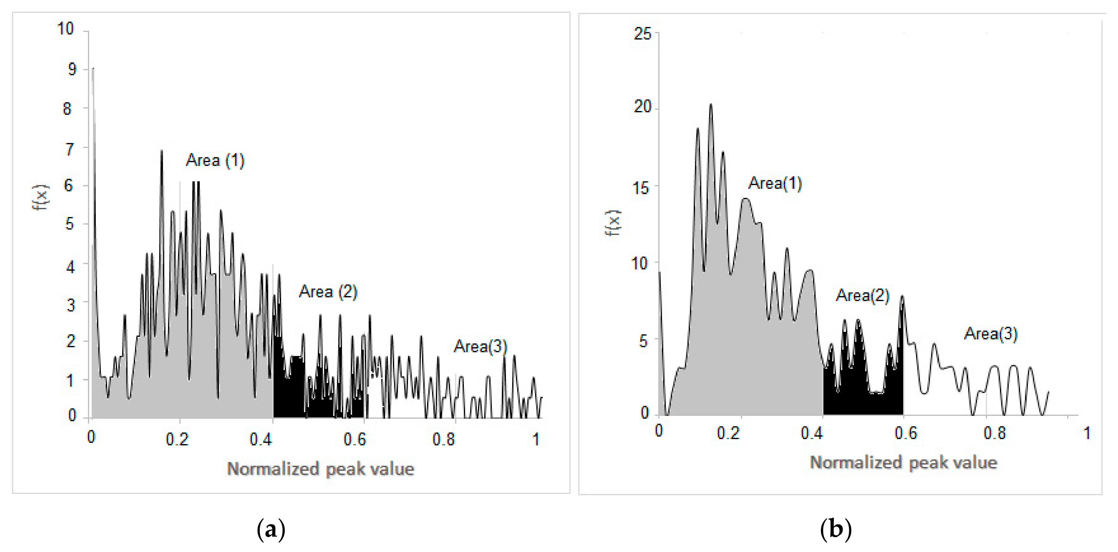
The local normalized peak values of IE signals (Y axis) in 3D matrix can also be used for IE classification. Figure 8 shows the frequency of signal’s peak values, which were normalized to 1 for slabs 4. The area under curve can be segmented to three areas:

▪

Area 1: normalized local peaks are between 0.005 and 0.4, with small local peaks compared to the absolute maximum.

▪

Area 2: normalized local peaks are between 0.4 and 0.6, with moderate local peaks compared to the absolute maximum.

▪

Area 3: normalized local peaks are between 0.6 and 0.95, with significant local peaks compared to the absolute maximum.

The area under each segment was calculated and summarized in

Table 4. Statistical result based on normalized peak for IE signals collected from defect part.

(a)
	Slab 1	Slab 2	Slab 3	Slab 4	Slab 5	Slab 6	Slab 7	Slab 8	Mean
Number of peaks 5 × 64	320	320	320	320	320	320	320	320	320
Area 1	4.19	4.50	4.30	4.26	4.74	4.87	4.85	4.69	4.55
Area 2	0.82	0.74	0.85	0.85	0.84	0.62	0.66	0.98	0.80
Area 3	1.42	1.26	1.23	1.53	1.17	1.50	1.37	1.21	1.33
(b)
	Slab 1	Slab 2	Slab 3	Slab 4	Slab 5	Slab 6	Slab 7	Slab 8	Mean
Number of peaks 5 × 188	940	940	940	940	940	940	940	940	940
Area 1	1.50	1.59	1.54	1.47	1.56	1.68	1.65	1.56	1.57
Area 2	0.39	0.25	0.26	0.26	0.32	0.24	0.24	0.32	0.29
Area 3	0.41	0.40	0.42	0.52	0.46	0.45	0.48	0.46	0.45

a,b for defect and sound data set, respectively. This approach revealed that the defected IE signals had higher value and more frequent local peak values compared to sound concrete. Moreover, one can observe more variability in the defected concrete as they were associated with four types of defects as opposed to sound IE data. These tables also show that the IE signals in each class of dataset, defect or sound, had similar statistical properties associated with their local peaks, while these properties were tangibly different from the other class. The result also showed that area (1) has the highest values compared to other domains. For example, most IE signals in both data set defect and sound had normalized local peaks lower than 0.4. However, these local peaks in sound set are concentrated in the small part of IE signal’s length near maximum points.

-

Start and stop time

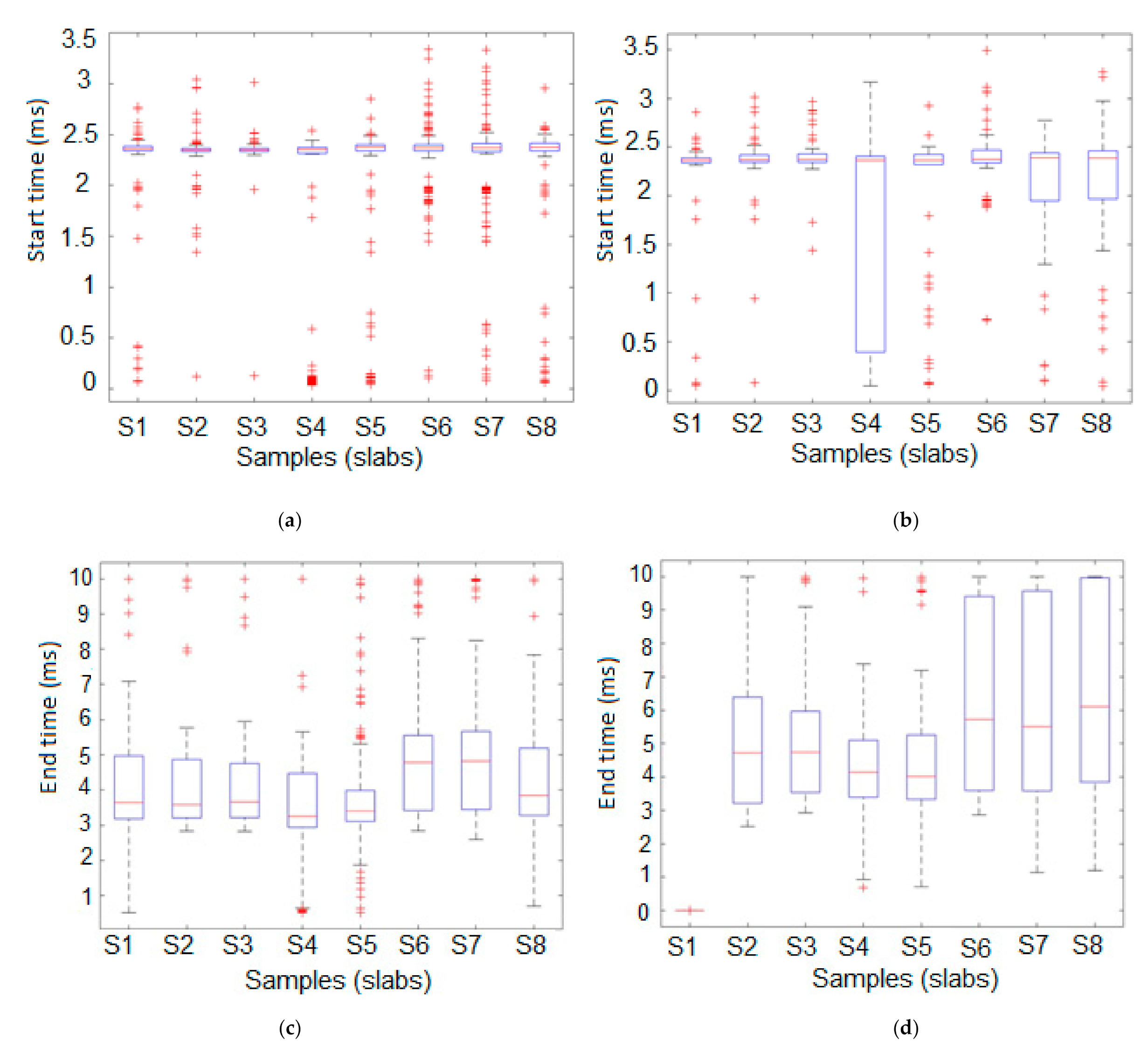
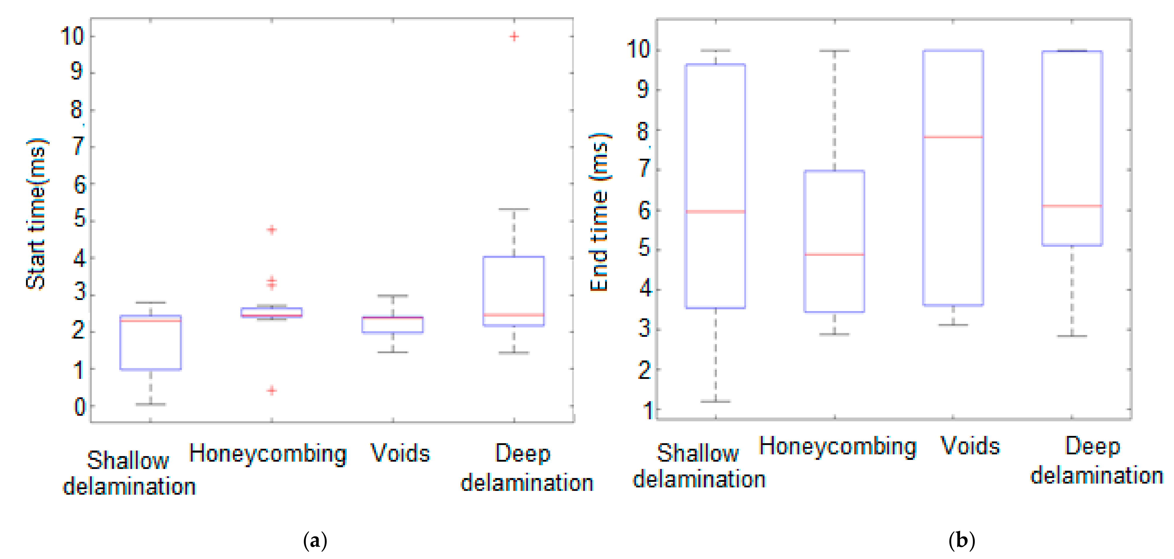
The start and end time of all processed IE signals were analyzed as another feature that can be used in Naïve Bayes for IE classification. Figure 9 shows the box plot for two data sets (defect and sound concrete).

As seen, the sound concrete showed less variability compared to defected concrete in terms of start and stop time of processed IE signals. The center of each box in these figures indicates the median, while the top and bottom bounds of them were the 25th and 75th percentiles, respectively. The end time seems to provide a better mean for classification compared to the stop time.

-

Defect type and histogram

The investigated slabs had four types of artificial defects, which were shown to affect the shape of the histogram and fitted distributions to the length of the processed IE as seen in Figure 10. The proposed IE signals collected from deep delamination and sound group are slightly similar to each other in terms of signal length. Therefore, it cannot be used for proper classification of IE signals. On the other hand, the start and end time of the processed IE signals showed more promise for classification detection, especially for deep delamination.

The length of the 80% preprocessed IE signals was collected from shallow delamination and void ranging from 100 to 1000 points. It ranged from 0 to 600 points for most of the IE data collected from deep delamination and honeycombing, and the mathematical code did not truncate 16% of the IE data due to multiple peaks or their unusual shape. The length of the 75% of the preprocessed IE signals is between 100 to 455 and the mathematical code cannot split 30% IE signals due to multiple peaks. Figure 10 also shows that the differences between the lengths of the IE signals collected from artificial defects could be related to the location, boundary conditions, or depth of the defect position.

Table 5. Probability result for preprocessed IE signal length based on defect type.

Parameters	Shallow Delamination	Honeycombing	Voids	Deep Delimitation	Mean
Number of data	128	128	128	128	128
Mean value	551	330	380.29	338	399
Coef. of Variance	0.90	1.45	1.20	1.5	1.26
Percentile 10%	117	95.9	113.2	99.3	106
Percentile 25%	175.75	114.25	132.5	110.25	132
Percentile 50%	415	146.5	201	134.5	224
Percentile 75%	900.5	234	473	213	455
Percentile 90%	1716.25	1861	1727	1962	1816
Best probabilistic fit	Fatigue life 3P	Pearson 5 3P	Burr	Logistic	----
f(x) for 0–370 points	0.42	0.78	0.70	0.80	0.67
f(x) for 370–900 points	0.30	0.04	0.10	0.02	0.11
f(x) for 900–1600 points	0.18	0.01	0.06	0.02	0.06
f(x) for 1600–2000 points	0.52	0.12	0.11	0.15	0.22
f(x) for unusual type	0	0.005	0.03	0.01	0.0125

shows the effect of the type of artificial defects on the shape of the histogram and fitted distributions in terms of their type; mean, and standard deviation of the IE lengths. According to Table 5, the IE signals collected from honeycombing and deep delamination had the least lengths in the prepressed signals.

This effect of type of delamination can be seen in the start and stop time as seen in Figure 10. The time interval of the prepossessed IE signals can be obtained with using this figure.

About 50% preprocessed IE data collected from shallow delamination had distinguished points before 2.5 ms. However, preprocessed IE signals collected from sound area do not have distinguished peaks before 2.5 ms. In addition, 50% preprocessed IE signals collected from shallow delamination had distinguished points in time interval between 6 to 10 ms. For deep delamination, the start points of 50% prepossessed IE data collected from deep delamination was between 2.6 and 4.2 ms, which were different from those data collected from sound regions. The start points of preprocessed IE data collected from sound concrete were approximately 2.5 ms. There was an overlap between 50% preprocessed IE data collected from honey becoming and preprocessed IE data collected from sound area. The start and end time of 50% prepressed IE signals collected from honey becoming was between 2.5 and 5 ms. As Figure 10 shows, there were overlaps between some part of prepressed IE data collected from void and preprocessed IE data collected from sound area in terms of sampling time interval.

3.2. Probability Classifier to Make Predicted Models Based on the Feature of IE Signals

Figure 11 shows the class of each data set, which was predicted using Naïve Bayes models and input layers. This model was able to predict the probability of present defects in the bridge using feature of signals, independently. Among all classifier approaches, Naïve Bayes models are applicable to IE data, since we can see the relationship between features and predicted surface, simultaneously.

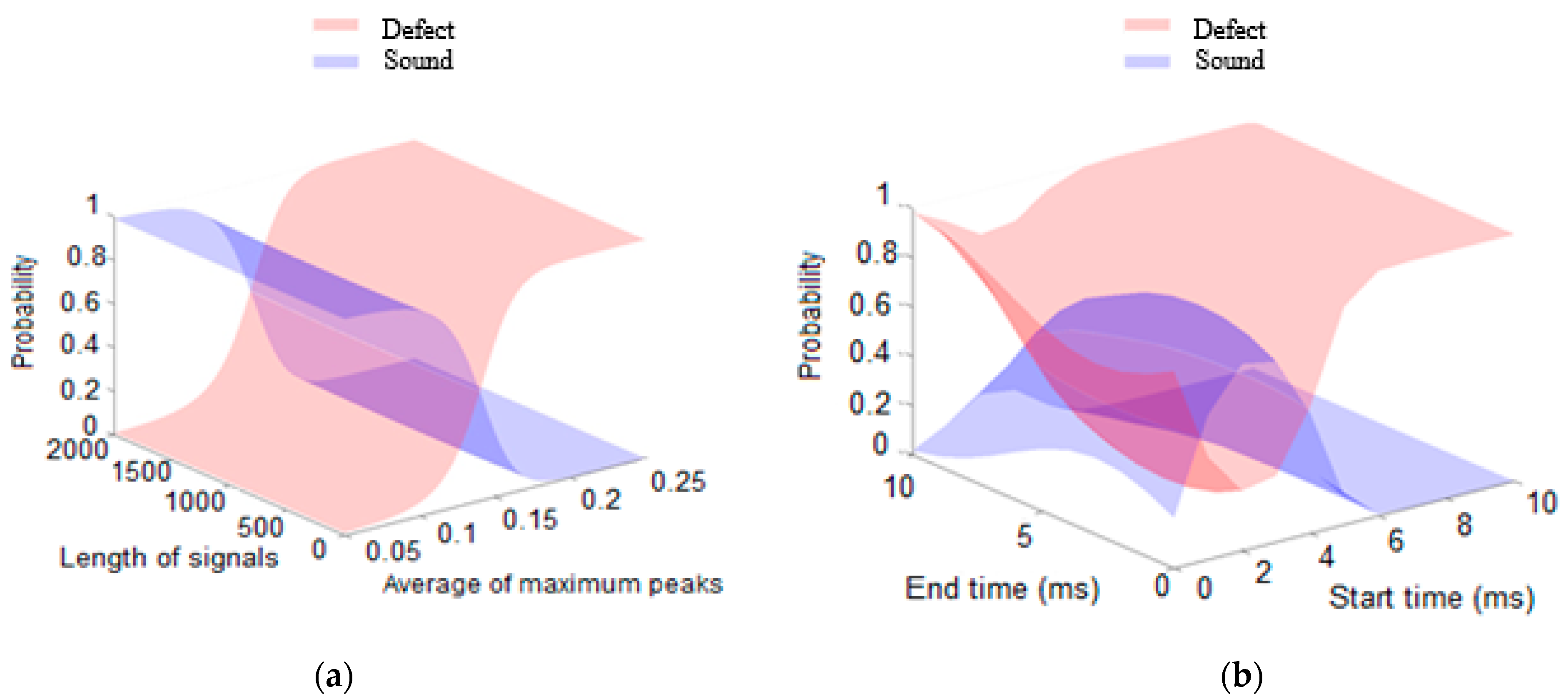
The relationship between average of maximum local peak, length of signals, end and start time of preprocessed signals and output layers (defect or sound area) can be obtained by using this method. It demonstrates how these two-input variables (length of signals or maximum peak) could influence the output layers in all slabs. Figure 12a,b demonstrate the probability of occurrence defect and sound regions based on nature of two independent variables.

It was made apparent that the length of the IE signals and normalized peak values influenced the results in the output layers of Naïve model (defect or sound) in all slabs. As Figure 11a shows, the IE signals collected from defect area has more distinguished peak. Therefore, increasing the amount of peak in signals leads to increase the probability of defect surface, which means, it is more likely the IE signals collected from defect area. In contrast, if normalized peaks in IE signals was reduced, it would lead to an increase in the probability of detection in sound surface. The probability result over normalized peak values and average of maximum peak showed to be higher in signals associated with defects compared to the ones associated with sound regions. This can be explained by the fact that signals collected from sound regions returned to the surface after hitting the bottom of specimens (backwall reflection). Therefore, the echo is in sound regions propagated through a longer path compared to the IE signals collected from the defect area. This also results in more dissipation of energy in the structure; which led to smaller values of local peaks in the sound region. Moreover, the IE signal collected from defect areas has larger normalized peaks because the data signals have two or more peaks due to the seismic wave encounter with the defects. The length of IE signals collected from the sound region was lower than the defect region, and the energy of IE signals in the sound set was more concentrated in certain time ranges without shifting energy to other part of signals. So, the processed IE signals collected from defect part has higher end time.

Figure 11b shows the relationship between end time, start time, and the occurrence probability of defect or sound regions. The variation of defect surface is related to the end time of signals such that the variation of surface of defect was increased when the end time of IE signal was between 5 to 10 ms. However, the sound surface was more variable when the end time of IE signal is between 2 to 4 ms. Based on the investigation it can be said:

-

The probability of the defect occurring ranges from 0.6–1 if the IE signal is truncated before 2 ms ($\mathrm{end} \mathrm{time} \mathrm{of} \mathrm{preprocessed} \mathrm{IE} \mathrm{signal} <\left(\frac{\mathrm{End} \mathrm{time} \mathrm{of} \mathrm{raw} \mathrm{IE} \mathrm{signal}}{10}\right)$).

-

The probability of the defect occurring ranges from 0.6–1 if the IE signal is truncated before 5 ms$(\mathrm{end} \mathrm{time} \mathrm{of} \mathrm{preprocessed} \mathrm{IE} \mathrm{signal}>\left(\frac{\mathrm{End} \mathrm{time} \mathrm{of} \mathrm{raw} \mathrm{IE} \mathrm{signal}}{2}\right))$.

-

The probability that the defect occurs is between 0.8–1 if the average of maximum peak of IE signal are higher than 0.16$.$

-

The probability of the defect occurring ranges from 0.1–0.2 if the IE signal is truncated between 2 and 4 ms.

-

The length of 90% of the preprocessed IE signals from the sound regions concluded 210 points within 2.5 and 3.5 ms. However, the length of 75% of preprocessed IE signals was concluded more than 400 points in the defect dataset, which is within 2.5 and 10 ms.

-

Probability classifier to make predicted models based on the estimated thickness and end time of preprocessed IE signals

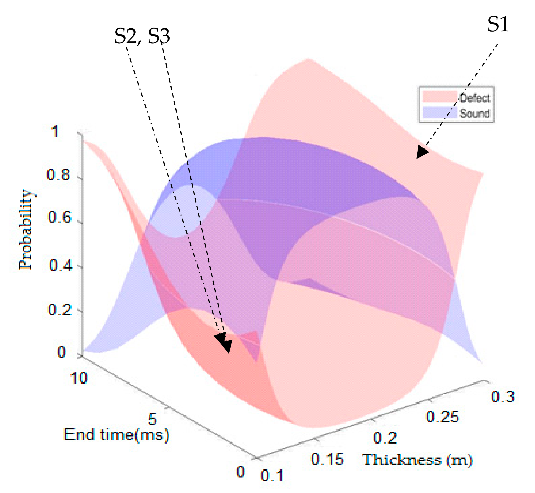
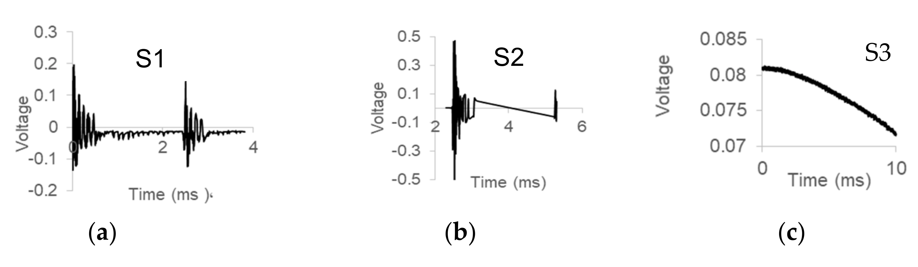
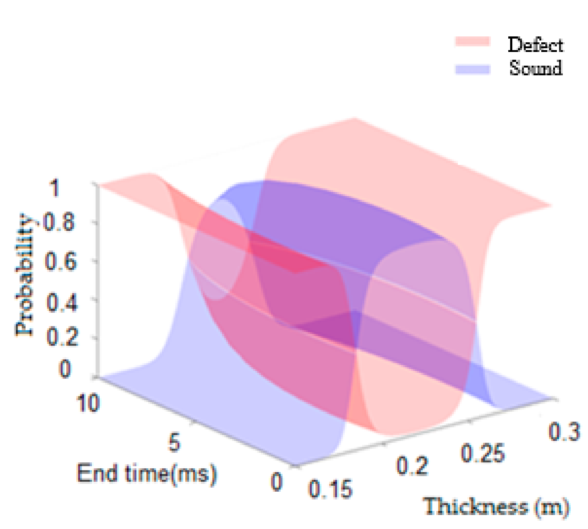
In this section, the probability classifier approach, the IE data of sound regions, and Equation (1) were used to evaluate the frequency spectrum analysis method. The estimated thickness from each IE signal, which was obtained from frequency approach, was added to the other features to generate probability of detection as seen in Figure 12 and Figure 13. As it is clear in this figure, employing the data of the sound dataset can provide an appropriate prediction of the slab thickness amount, which ranges between 0.15–0.3 associated with a 100% detection rate with some exceptions (see S1, S2, S3 as examples). The thickness for defected signals were outside the range of 0.15–0.25. It is important to note that preprocessed IE signals with an end time less than 2 ms are not suitable to predict the slab thickness.

All eight slabs had identical condition during construction; however, the IE data collected from different slabs were not the same because the estimated thickness in not the same between slab (7) and slab (8). The time range of the prepossessed IE signals and the peak values of the IE signals are different for each slab. Based on previous research [27], this difference could be due to the different mix design, moisture condition, and the operator’s preferences when collecting the data. As can be clearly seen in Figure 12 and Figure 14, the IE signals collected from slab (8) can estimate thickness more accurately. The estimated thickness is between for slab 8 was between 0.2 m and 0.25 m; however, this value was between 0.15 m and 0.3 for slab (7). This inconsistency shows the importance of investigating IE in the time domain to produce more accurate thickness estimation.

The purpose of this section was to obtain the 3-D surface as evidence to show how to detect defect area in IE signals in both time and frequency domains. Moreover, atypical IE signals collected from sound or the defect area can be obtained using the 3-D surfaces. For example, 10% of IE signals in sound data collected from slab (8) is not usable to estimate slab thickness.

-

Pearson coefficient

Pearson coefficient was used to evaluate the correlation between two variables scaled from −1 to +1. A coefficient of 1 indicates that two datasets are significantly correlated, whereas -1 indicates that two datasets are in a strongly negative relationship [28]. Pearson confidence coefficient is more common to evaluate the similarity between two objects in a large statistical dataset. So, the similarity between the slabs was determined based on the result of the frequency approach and the features of the raw IE signals in the time domain.

Table 6. Pearson coefficient to evaluate similarity among slabs.

	Slab 1	Slab 2	Slab 3	Slab 4	Slab 5	Slab 6	Slab 7	Slab 8
Slab 1	1	0.8437	0.7359	0.7070	0.4921	0.7891	0.6845	0.5638
Slab 2	0.8437	1	0.7167	0.8763	0.6200	0.6890	0.8553	0.7167
Slab 3	0.7359	0.7167	1	0.9568	0.6368	0.6559	0.8732	0.7417
Slab 4	0.7070	0.8763	0.9568	1	0.7024	0.7399	0.8485	0.7926
Slab 5	0.4921	0.6200	0.6368	0.7024	1	0.6442	0.7456	0.9543
Slab 6	0.7891	0.6890	0.6559	0.7399	0.6442	1	0.6790	0.6710
Slab 7	0.6845	0.8553	0.8732	0.8485	0.7456	0.6790	1	0.8364
Slab 8	0.5638	0.7167	0.7417	0.7926	0.9543	0.6710	0.8364	1

summarizes the Pearson coefficient for all slabs obtained to examine the similarity between the IE signals in terms of frequency response among all slabs. According to Table 6, slabs 1, 2, 3, and 4 are similar to each other, and slabs 5, 7, and 8 are more similar to each other. Finding similarity index between slabs can help a user of IE device to classify IE data more accurately.

Based on the result of statistical model, boxplots, probability classifier, and Pearson coefficient it was concluded that slabs (5), (7), and (8) were similar to each other and slabs (1), (2), (3), and (4) were more similar, which will be investigated in future studies. The proposed features in this study can be directly applied to IE collected by different data collection settings and devices as they were extracted from process IE signals.

-

Comparison

In a different study, IE signals were used to build a prediction method without controlling the quality of IE signals or extracting atypical IE signals, which could lead to errors to predict defect area [11,20,29,30]. The result of the current study shows about 10% of IE signals do not have a normal shape in the IE dataset used in this study. Therefore, the authors suggested to extract atypical signals before creating the prediction method, which can reduce the estimation errors by 10%. The proposed method can be effectively used for IE signal quality control during inspections.

Using the proposed processing, IE signals can be used for more accurate estimation of concrete decks. In a previous study, the error of the estimated thickness was between 5 and 15% when using two datasets with 512 IE signals collected from slabs without defect area [31]. In our study, all slabs contained four types of artificial defects including shallow delamination, deep delamination, honeycombing, and voids. The boundary conditions at the interface between the defect and surface of concrete leads to an increase in the error of the estimated thickness. This error is 10%, considering several of IE data used in this paper did not have the proper quality (unusual signals). Another merit of this investigation was to develop a method to find unusual IE signals in a large dataset with 2016 IE signals before estimating thickness.

In recent studies, the frequency approach and machine learning method were used to interpret IE signals, separately [11,20]. However, in this study, the Naive Bayes classifiers approach was used to detect defects for the first time by using IE signals in both time and frequency domains. The proposed pre-processing method reduced the classification error when applied on the IE raw data. Therefore, the result of classification using the proposed features in this study can be coupled with the conventional peak frequency method to consider both time domain and frequency domain characteristics.

4. Conclusions

In this investigation, a set of features are proposed which can be used to classify impact echo data using their time series for the first time. To do this, the preprocessing filtering approach was used to modify raw impact echo signals for better feature extraction including distinguished peaks, their corresponding time, and the length. The probability density functions for these features were obtained for IE data collected from eight laboratory-reinforced concrete specimens with artificial defects. Naive Bayes classifiers were also employed to classify defect and sound regions based on a set of features in IE signals. The results showed that distinguished peak points, their corresponding time, and length of the processed IE signals were proper features to classify IE data of defect concrete compared to the sound concrete. Therefore, each dataset “Defect” or “Sound” can be detected by a set of unique statistical features.

The main takeaways of this paper are as follow, based on the IE data used in this study:

-

The result of statistical model and probability classifier shows 10% of the IE data collected from the sound area are unusable for estimating thickness using the frequency method because of unusual shape.

-

The result over defect type of IE signals showed the detection of shallow delamination and deep delamination as defect types were more straightforward than the other two types of defect types, as 50% of the preprocessed IE data collected from shallow delamination had distinguishable points before and after 2.5 ms in the processed signals. However, the preprocessed IE signals collected from the sound area had no distinguishable peaks before 2.5 ms.

-

The proposed features in this study can be directly applied to IE collected by different data collection settings and devices as they were extracted from process IE signals. The result of classification using the proposed features in this study can be coupled with the conventional peak frequency method to consider both time domain and frequency domain characteristics.

-

Using the preprocessing approach results in obtaining more information about the number of peaks, the peak values, and the corresponding time range, which improved the classification accuracy.

-

Using the preprocessing approach and frequency methods leads to a better understanding of IE data, which can help the user distinguish the defect area. In addition, some data in two datasets (sound or defect) do not follow the common patterns in the dataset, which can be separated by the probability method.

-

With using the proposed probability, probability classifier, and preprocessing approach, it is possible to increase the rate of the frequency analyses.

References

- Ghomi, M.T.; Mahmoudi, J.; Darabi, M. Concrete plate thickness measurement using the indirect impact-echo method. Nondestruct. Test. Eval. 2013, 282, 119–144. [Google Scholar] [CrossRef]
- Edwards, L.; Bell, H.P. Comparative evaluation of nondestructive devices for measuring pavement thickness in the field. Int. J. Pavement Res. Technol. 2016, 9, 102–111. [Google Scholar] [CrossRef] [Green Version]
- Yeh, P.-L.; Liu, P.-L. Imaging of internal cracks in concrete structures using the surface rendering technique. NDT E Int. 2009, 42, 181–187. [Google Scholar] [CrossRef]
- Carino, N.J.; Sansalone, M. Flaw detection in concrete using the impact-echo method. In Bridge Evaluation, Repair and Rehabilitation; Springer: Berlin/Heidelberg, Germany, 1990; pp. 101–118. [Google Scholar]
- Kee, S.H.; Gucunski, N. Interpretation of flexural vibration modes from impact-echo testing. J. Infrastruct. Syst. 2016, 223, 04016009. [Google Scholar] [CrossRef]
- Abdelkhalek, S.; Zayed, T. Comprehensive inspection system for concrete bridge deck application: Current situation and future needs. J. Perform. Constr. Facil. 2020, 34, 03120001. [Google Scholar] [CrossRef]
- Muldoon, R.; Chalker, A.; Forde, M.C.; Ohtsu, M.; Kunisue, F. Identifying voids in plastic ducts in post-tensioning prestressed concrete members by resonant frequency of impact–echo, SIBIE and tomography. Constr. Build. Mater. 2007, 213, 527–537. [Google Scholar] [CrossRef]
- Colla, C.; Lausch, R. Influence of source frequency on impact-echo data quality for testing concrete structures. NDT E Int. 2003, 364, 203–213. [Google Scholar] [CrossRef]
- Nguyen, T.D.; Tran, K.T.; Gucunski, N. Detection of bridge-deck delamination using full ultrasonic waveform tomography. J. Infrastruct. Syst. 2017, 232, 04016027. [Google Scholar] [CrossRef]
- Yeh, P.L.; Liu, P.L.; Hsu, Y.Y. Parametric analysis of the impact-echo phase method in the differentiation of reinforcing bar and crack signals. Constr. Build. Mater. 2018, 180, 375–381. [Google Scholar] [CrossRef]
- Dorafshan, S.; Azari, H. Deep learning models for bridge deck evaluation using impact echo. Constr. Build. Mater. 2020, 263, 120109. [Google Scholar] [CrossRef]
- Schubert, F.; Wiggenhauser, H.; Lausch, R. On the accuracy of thickness measurements in impact-echo testing of finite concrete specimens––Numerical and experimental results. Ultrasonics 2004, 421, 897–901. [Google Scholar] [CrossRef]
- Schoefs, F.; Abraham, O. Probabilistic evaluation to improve design of impact–echo sources. Transp. Res. Rec. 2012, 23131, 109–115. [Google Scholar] [CrossRef] [Green Version]
- Igual, J.; Salazar, A.; Safont, G.; Vergara, L. Semi-supervised Bayesian classification of materials with impact-echo signals. Sensors 2015, 155, 11528–11550. [Google Scholar] [CrossRef]
- Pagnotta, A. Probabilistic Impact-Echo Method for Nondestructive Detection of Defects around Steel Reinforcing Bars in Reinforced Concrete. Ph.D. Thesis, Civil Engineering in the Graduate College, University of Illinois at Urbana-Champaign, Champaign, IL, USA, 2018. [Google Scholar]
- Rashidi, M.; Azari, H.; Nehme, J. Assessment of the overall condition of bridge decks using the Jensen-Shannon divergence of NDE data. NDT E Int. 2020, 110, 102204. [Google Scholar] [CrossRef]
- Ye, J.; Kobayashi, T.; Iwata, M.; Tsuda, H.; Murakawa, M. Computerized hammer sounding interpretation for concrete assessment with online machine learning. Sensors 2018, 18, 833. [Google Scholar] [CrossRef] [PubMed] [Green Version]
- Cho, Y.S.; Hong, S.U.; Lee, M.S. The assessment of the compressive strength and thickness of concrete structures using nondestructive testing and an artificial neural network. Nondestruct. Test. Eval. 2009, 243, 277–288. [Google Scholar] [CrossRef]
- Sadowski, Ł.; Hoła, J.; Czarnecki, S. Non-destructive neural identification of the bond between concrete layers in existing elements. Constr. Build. Mater. 2016, 127, 49–58. [Google Scholar] [CrossRef]
- Dorafshan, S.; Azari, H. Evaluation of bridge decks with overlays using impact echo, a deep learning approach. Autom. Constr. 2020, 113, 103133. [Google Scholar] [CrossRef]
- Zheng, Q.; Yang, M.; Yang, J.; Zhang, Q.; Zhang, X. Improvement of Generalization Ability of Deep CNN via Implicit Regularization in Two-Stage Training Process. IEEE Access 2018, 6, 15844–15869. [Google Scholar] [CrossRef]
- Shen, J.; Li, S.; Jia, F.; Zuo, H.; Ma, J. A deep multi-label learning framework for the intelligent fault diagnosis of machines. IEEE Access 2020, 8, 113557–113566. [Google Scholar] [CrossRef]
- Adam, A.; Shapiai, M.I.; Tumari, M.Z.M.; Mohamad, M.S.; Mubin, M. Feature Selection and Classifier Parameters Estimation for EEG Signals Peak Detection Using Particle Swarm Optimization. Sci. World J. 2014, 2014, 1–13. [Google Scholar] [CrossRef] [PubMed] [Green Version]
- Schittkowski, K. EASY-FIT: A software system for data fitting in dynamical systems. Struct. Multidiscip. Optim. 2002, 23, 153–169. [Google Scholar] [CrossRef]
- Friedman, J.; Hastie, T.; Tibshirani, R. The Elements of Statistical Learning; Springer Series in Statistics; Springer: New York, NY, USA, 2001; Volume 1. [Google Scholar]
- Sengupta, A.; Ilgin Guler, S.; Shokouhi, P. Interpreting Impact Echo Data to Predict Condition Rating of Concrete Bridge Decks: A Machine-Learning Approach. J. Bridge Eng. 2021, 268, 04021044. [Google Scholar] [CrossRef]
- Sutan, N.M.; Jaafar, M.S. Defect Detection of Concrete Material by Using Impact Echo Test. J. Nondestruct. Test. 2003, 8, 1–5. [Google Scholar]
- Garren, S.T. Maximum likelihood estimation of the correlation coefficient in a bivariate normal model with missing data. Stat. Probab. Lett. 1998, 38, 281–288. [Google Scholar] [CrossRef]
- Epp, T.; Svecova, D.; Cha, Y.J. Semi-Automated air-coupled impact-echo method for large-scale parkade structure. Sensors 2018, 18, 1018. [Google Scholar] [CrossRef] [PubMed] [Green Version]
- Zhang, J.K.; Yan, W.; Cui, D.M. Concrete condition assessment using impact-echo method and extreme learning machines. Sensors 2016, 16, 447. [Google Scholar] [CrossRef] [PubMed]
- Baggens, O.; Ryden, N. Systematic errors in Impact-Echo thickness estimation due to near field effects. NDT E Int. 2015, 69, 16–27. [Google Scholar] [CrossRef] [Green Version]
Figure 1.
Details of the slabs.
Figure 2.
Naive Bayes classifiers model and the features (a) for preprocessed IE signals, (b) for preprocessed IE signals, and result of frequency approach based on raw IE signals.