1. Introduction
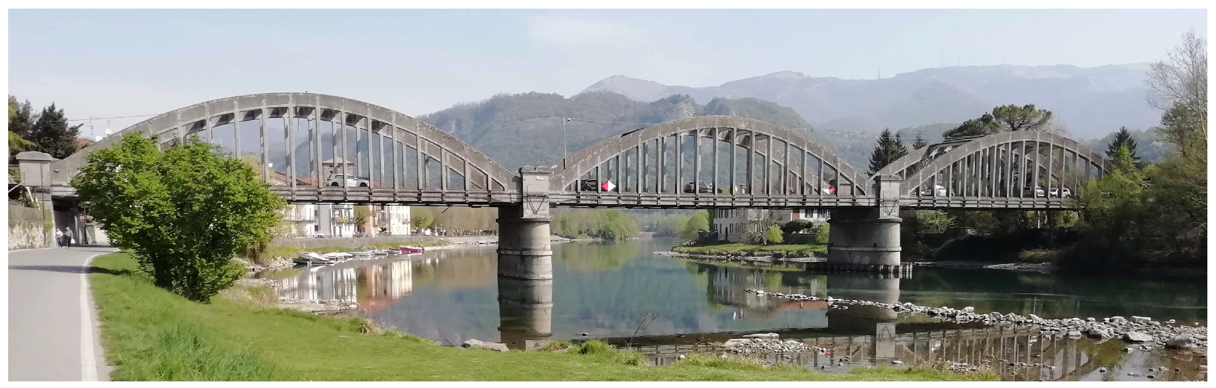
A fundamental step toward achieving an efficient and reliable updated model identification of important infrastructures, such as a strategic aged road bridge, is constituted by producing an appropriate signal processing of acquired response data. The case study investigated in the present article is that of specific road infrastructure, namely a historical reinforced concrete three-span arch bridge, the Brivio bridge [
1]. The bridge is located between Brivio and Cisano Bergamasco (province of Lecco and Bergamo, respectively, Lombardia region, Northern Italy, near Milano), over the Adda river, flowing out of the Lecco branch of Como Lake and going down toward the Po valley. Built at the end of World War I in 1917 (and seemingly tested right away before opening by a column of military vehicles [
2]), the bridge presents a significant historical and structural value, and currently preserves its full functionality, with heavy traffic, daily, then keeping a fundamental, actually crucial, infrastructural role in the local region.
The bridge has been the subject of a comprehensive investigation in the recent years [
3], toward assessing its current functioning conditions, based on an experimental campaign of response data acquisition and processing, with the target of developing integrated methodological approaches of post-processing analysis, based on Heterogeneous Data Fusion [
4,
5,
6], non-empirical, i.e., algorithmic, FEM model updating [
7,
8], and signal denoising [
9,
10,
11].
The present article is part of such an integrated investigation and focuses on some aspects of detail, within the signal processing analysis of specific acquired vibrational data from the deck of the bridge (by standard wired accelerometer sensors), and on their possible interpretation, toward achieving proper confidence, in the evaluation of the present structural behaviour of the bridge. Accurate, detailed processing of the whole acceleration response signals collected during a three-day recording campaign (occurred between 11 and 13 June 2014) carried out on the bridge is foreseen, after the first-order processing of main data [
7], by using mere signal processing methodologies (see, e.g., [
12,
13,
14,
15,
16]). Overall, the comprehensive tests were performed by employing different instrumentation systems and sensors, such as classical uniaxial wired piezoelectric accelerometers, low-cost wireless sensors, total stations and a laser scanner, with a global target also on inspecting all three bridge spans, for operational dynamic testing of the structure under current traffic load conditions [
3].
In particular, with one main goal to identify the dominant frequencies from the signals recorded by vertical accelerometer sensors placed on the deck of the bridge, a comprehensive methodology of data analysis is herein set, and thoroughly performed, on the achieved acceleration response data. Particularly, the vibration content and the structural significance of the acquired signals are investigated, according to classical signal processing techniques. The analysis is systematically developed on the full record of each channel. Specifically, the plot of the full acceleration record is analysed and a time-domain analysis is performed first, by determining the maximum positive, minimum negative and Root Mean Square (RMS) values; the statistical analysis is developed by calculating the distribution of the instantaneous values and the positive and negative peaks, adding correlation and spectral analyses. As a first refinement, three record sub-windows with a limited duration and a high level of response are selected, along the full record. The autocorrelation function, the “spectrum” (Fourier amplitude) and the cross-correlation function between the selected channel and each other are computed, according to classical signal processing strategies [
15,
16].
In order to comply with the results obtained from such a detailed first-order signal processing analysis, it is then envisaged to adopt further refined techniques, for the statistical analysis of non-stationary data. Specifically, a Wavelet technique (see, e.g., [
17,
18]) is selected, as an efficient approach for this purpose. Being already successfully applied in the application fields of damage identification (see, e.g., [
19,
20,
21]) and signal denoising (see, e.g., [
9,
10,
11,
22]), a Wavelet analysis can be specifically considered in bridge signal processing, as e.g., proposed in [
23,
24,
25,
26,
27,
28,
29]. It is here applied to the same two channels of each side of the central span of the bridge only, assuming that the outcomes could easily be extended to the channels of the other two spans. A further devoted analysis is discussed, through AutoRegressive Moving Average (ARMA) models (for a classical theoretical reference, see, e.g., [
30]), which are nowadays under continuous investigation, within innovative applications in the SHM area (see, e.g., [
31,
32,
33,
34,
35,
36]).
Overall, this sets a comprehensive methodology for a consistent signal processing analysis of the collected response recordings. The aim of the present research is to find out a procedure for effective processing of experimental signal data displaying stochastic non-stationary characteristics. This choice is justified in order to adopt already available and sound tools to obtain a low cost and reliable self-implemented methodology for SHM purposes. Moreover, it comes then to support possible first interpretations of the originally conceived and current recorded structural behaviour of the bridge. On the basis of the achieved information, some conjectures on the actual mechanical response of the structure are advanced, specifically in terms of the potential influence of the supporting parabolic arches and of an apparent display of non-linear behaviour.
The paper is organised as follows.
Section 2 briefly recalls the main features of the experimental campaign and the measurement setup, to provide data collection and to allow for initial global processing of the registered signals.
Section 3 develops the first set of refined analyses on the acquired signals, on the basis of further specific classical signal processing techniques.
Section 4 considers a Wavelet analysis, in order to additionally inspect the set of acquired data and to open up the way to a possible interpretation of the structural behaviour of the bridge. With the same scope,
Section 5 supplementary proposes an application of an ARMA approach, toward the appreciation of consistent outcomes of the conceived and current mechanical response of the bridge structure, with respect to the possible influence of the supporting arches and to an apparent non-linear behaviour. This is then outlined in
Section 6, proposing some first structural interpretations on the outcomes of the signal processing methodology and analyses, and gathering a synopsis of the deciphered fundamental frequencies of the bridge. At last, closing
Section 7 summarizes the obtained results and outlines the main remarks of the study, both on the source developed methodological approach of signal processing, with validity also in general terms, and on the achieved specific resulting outcomes, and on the interpretation of the actual structural response of the bridge.
2. Data Collection and First Signal Processing
In order to properly illustrate the data collection stages, brief descriptions of the Brivio bridge (
Figure 1) from a structural concept standpoint and of the carried out experimental campaign are here provided (with source reference and further information that may be accessed in [
3,
4,
5,
7]).
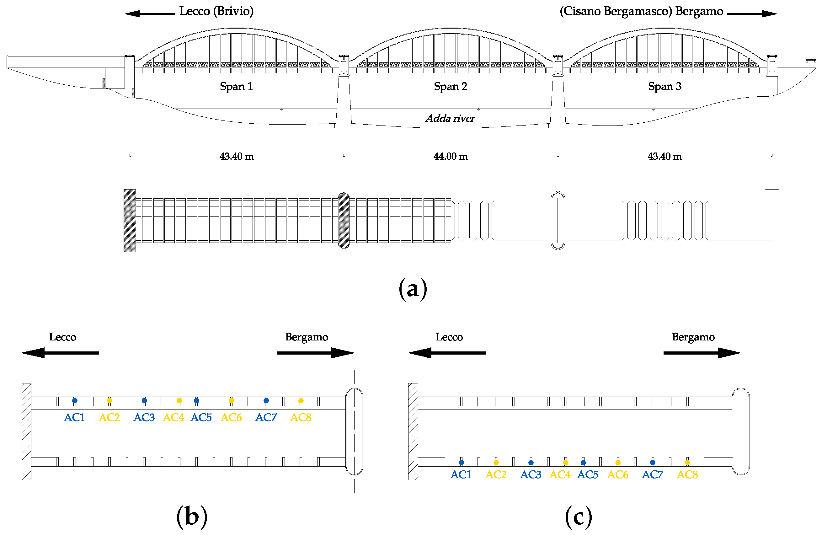
The reinforced concrete road bridge, over the Adda river, consists of three arched spans, supported by characteristic twin parabolic arches hanging underneath the straight deck, and presents a full symmetry with respect to its mid-longitudinal plane [
1,
2,
7]. The average height of the deck is about 8 m above water level. The central span, bearing on two pillars on the river bed, is 44 m long, while the lateral spans, connected to the river banks are 43.4 m long, summing up to a total length of 130.8 m. The road deck is 9.2 m wide, designed for two roadway lanes, sided by two cantilever sidewalks, each 0.8 m wide. In each span of the bridge, the deck includes two main longitudinal girders (section 0.45 m × 1.00 m), placed at a respective transverse distance of 8.60 m, joined by two further secondary beam elements (section 0.20 m × 0.55 m) installed at a distance pairing to 2 m, symmetrically located with respect to the vertical longitudinal plane of the bridge; between this girder system, transverse beam connections (section 0.30 m × 0.75 m) are set, approximately every 2.30 m. Globally, the grid structure supports a reinforced concrete slab, with a thickness equal to 0.15 m. The parabolic arches of the bridge are built on a 42.80 m span, coupled with a rise of 8.00 m. The cross-section of each arch structural element exhibits a rectangular shape, defined by a constant width (0.60 m) and a variable height (from 1.25 m, at the midsection, to 1.37 m at the impost). The whole profile of each arch is symmetric with respect to the vertical axis at half span. Each arch is connected to the corresponding other on their upper central part by eight transverse beams and to the bridge deck through a system (considered at each side, at each span) of sixteen reinforced concrete hangers, with a rectangular cross-section (0.32 m × 0.60 m). The intermediate supports of the spans, inside the river bed, are constituted by two concrete piers, provided with a tapered cross-section, showing maximum dimensions, at the base, equal to 12.8 m, in the transverse direction of the bridge, and to 3.8 m measured in the longitudinal direction. The pier foundation system is set on forty-eight reinforced concrete piles (square cross-section with 0.35 m side), driven into the river bed, ranging from 13 m to 16 m in depth. Above both the intermediate piers and the abutments, supporting reinforced concrete slabs (height equal to 1 m) are placed.
Operational experimental campaigns were performed on the Brivio bridge between 11 and 13 June 2014. In order to carry out the tests, several instrumentation systems were adopted: ten uniaxial wired piezoelectric accelerometers, seven wireless sensors, four QDaedalus system total stations and a laser scanner, employed simultaneously for dynamic testing of the structure under current traffic loading conditions, defining diverse setups (see also [
4,
5]). In this first monitoring campaign and subsequent signal processing, the main focus was made on vertical vibrations, under regular traffic loading, as recorded by standard wired unidirectional accelerometers, placed on the deck of the bridge, to detect its main vibrational response characteristics. In this article, a global signal processing methodology and campaign are considered by analysing just the complete set of measurements provided by the vertical wired piezoelectric accelerometers placed on the whole deck structure, namely on the three spans, on their two lateral sides.
The set of accelerometers was placed on the bridge as a compound system constituted by: (
i) a 24-channel data acquisition system, comprising six NI 9234 4-channel dynamic signal acquisition modules (24-bit resolution, 102 dB dynamic range and anti-aliasing filters), connected to a remote computer provided with a storage unit; (
ii) uniaxial WR 731A piezoelectric accelerometers on the roadway deck, where each WR 731A sensor was capable of measuring accelerations up to 0.5 g, with a sensitivity of 10 V/g, and was connected with a short cable to a WR P31 power unit and amplifier. The sampling rate frequency for the data acquisition was equal to 200 Hz, according to the available instrumentation. With the aim of capturing both the bending and torsion responses, vertical accelerometers were placed on both sides of the bridge deck. The two employed setups are schematically depicted in
Figure 2. Per each setup configuration, two complete time series were recorded (whole time duration equal to 3600 s), to warrant a sufficiently large database of measurement from a statistical point of view.
A preliminary data analysis is performed, for each acceleration channel mounted on each span of the bridge, in the time and the frequency domain, to classify the type of the recorded vibration, irrespectively of its origin. In particular, a characteristic data processing is produced, along with the following steps, here schematically described to define a common methodological procedure developed in the whole set of analyses (see
Box 1 and following
Box 2 and
Box 3).
Box 1. Steps of the first systematic signal processing.
Each full response record is analysed and plotted in the time domain; then processed.
The maximum positive peak, the minimum negative peak and the Root Mean Square (RMS) value of the record are determined.
The distributions of the instantaneous, positive and negative peak values of the record are compared, respectively with the Gaussian distribution having the experimental RMS value and with the Rayleigh and Weibull distributions having the experimental median, to classify the statistical characteristics of the signals.
The autocorrelation function of significant records of the acquired response signals is calculated.
The Power Spectral Density (PSD) is evaluated by splitting the available record into 160 sub-records, consistently checking for resulting frequency resolution and random error.
Significant and resuming obtained results are hereinafter reported, where the comments are to be considered common to all the devised channels, regardless of the span, unless explicitly stated. It is worth observing that the monitored vibration is quite similar throughout the whole record. Moreover, the amplitude of the recorded ambient vibration is characterized by a succession of beats, probably generated by regular operational traffic of the vehicles (including trucks) passing onto the bridge.
Referring to the second and third steps of the procedure described above, relatively to the maximum and minimum peak value, together with the RMS value, a comparison is made between the experimental distributions of the values and the corresponding mathematical distributions. The typical distribution of the instantaneous and positive peak values is provided in
Figure 3. The following remarks can be drawn.
The instantaneous values do not follow a Gaussian (normal) distribution; more precisely, the experimental distribution is leptokurtic, because the kurtosis turns out to be greater than 3 (as referred to any univariate normal distribution) [
12].
The kurtosis indicates the extent to which probability is concentrated in the centre and especially the tails of the distribution rather than in the shoulders. Kurtosis indices are determined for each channel installed on Span 2 and are herein reported in
Table 1; their values describe a significant difference between the statistical distribution of experimental data and a Gaussian distribution, therefore requiring specific attention in subsequent structural identification and interpretations.
The peak signal values are not distributed as a Rayleigh distribution, while their distribution turns out quite similar to that of a Weibull distribution (continuous plots in
Figure 3c,d); this means that the probability to record peak values lower than the median of the peaks is higher than the one which could be obtained with a Rayleigh distribution.
Table 1.
Kurtosis values determined on the signals acquired by the channels installed on Span 2 (mid span on pillars within the river).
Table 1.
Kurtosis values determined on the signals acquired by the channels installed on Span 2 (mid span on pillars within the river).
| Channel | Upstream Side | Downstream Side |
|---|
| 1 | 13.88 | 18.83 |
| 2 | 18.33 | 17.29 |
| 3 | 18.74 | 21.05 |
| 4 | 37.57 | 20.05 |
| 5 | 33.31 | 23.08 |
| 6 | 17.57 | 24.37 |
| 7 | 14.45 | 14.37 |
| 8 | 11.90 | 14.60 |
From a mathematical standpoint, the probability density distribution of Weibull can be described by the following formula [
12]:
where
a is the peak value,
is the median of the peak values,
k is the parameter of the Weibull distribution and where, for
, the Weibull distribution coincides with the Rayleigh distribution. To further confirm the observations derived by the data presented in
Figure 3, the values of parameter
k are here calculated for each measuring channel installed onto the bridge and result to be equal when referred to the same span, i.e.,
for Span 1,
for Span 2,
for Span 3.
The inspection of results of further analyses in the time domain, determining the autocorrelation function for each recorded signal, extracts the following observations.
Considering Span 1: for Channels 1, 3, 6, on the upstream side and for Channels 1, 4, 5, 7, 8 on the downstream side, the autocorrelation function results to be typical of a narrow-band random signal; while for Channels 2, 4, 5, 7, 8 on the upstream side and for Channels 2, 3, 6 on the downstream side, the autocorrelation function shows more frequency spread, with respect to a narrow-band random signal. Moreover, there appears an evident dominance of just one frequency at 11.43 Hz for Channels 1, 3, 6 on the upstream side and for Channels 1, 4, 5, 7, and 8 on the downstream side.
Considering Span 2: for all Channels on the upstream side and for Channels 1, 3, 4, 5, 6 on the downstream side, the autocorrelation function results to be typical of a narrow-band random signal; while for Channels 2, 7, 8 on the downstream side, the autocorrelation function shows more frequency spread, with respect to a narrow-band random signal. Moreover, there appears an evident dominance of just one frequency at 6.05 Hz for Channels 4, 5 on the upstream side and at 11.80 Hz for Channels 2, 7, 8 on the downstream side.
Considering Span 3: for Channels 1, 2, 3, 6, 7, 8 on the upstream side and for Channel 1 on the downstream side, the autocorrelation function results to be typical of a narrow-band random signal; while for Channels 4, 5 on the upstream side and for Channels 2, 3, 4, 5, 6, 7, 8 on the downstream side the autocorrelation function shows a more frequency spread. A clear dominant frequency is present for Channels 1 and 7 on the upstream side, at 3.76 Hz and 11.60 Hz, respectively, and for Channel 1 on the downstream side at 12.50 Hz.
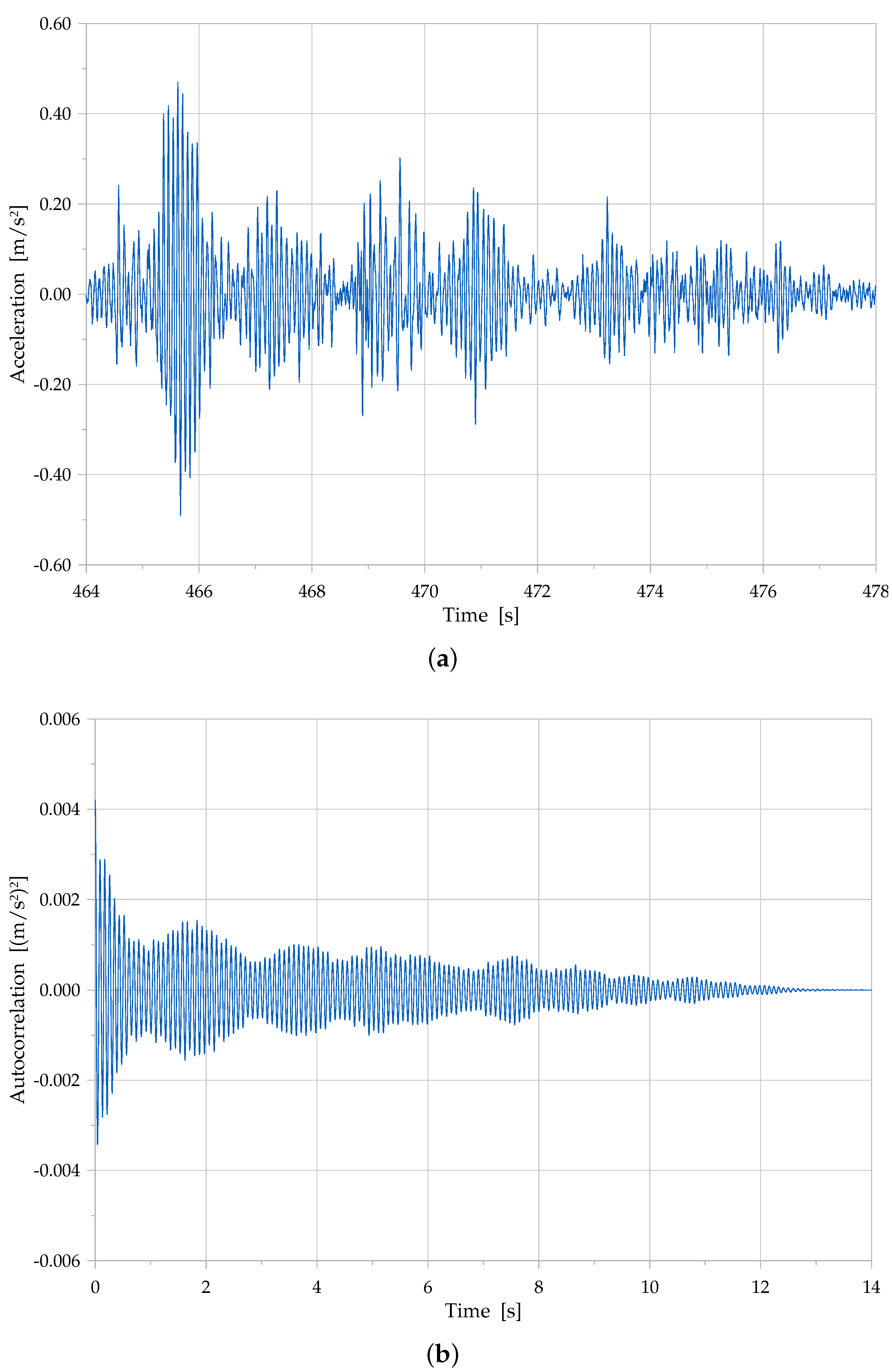
For illustrative purposes,
Figure 4 reports a typical acquired acceleration response signal (sub-record over a width of 14 s) and its autocorrelation function. This shows, from a statistical standpoint, that the recorded response signal displays a primary random nature, related to the expected dominating decaying behaviour shown by the autocorrelation function, also by the following beats of response. Such observation confirms the nature and quality of the recorded signal, ensuring the possibility to tackle the data within a signal processing analysis. Moreover, the additional oscillations and local peaks on the function, i.e., looking as carrier and modulation waves, may highlight the presence of some dominant frequencies of the structure or of their interactions, possibly related to combinations of the modes of the structure, as also related to the operational loading. Overall, the features that are observed look suitable to state that the signal seems appropriate for processing, in order to extract relevant information on the underlying mechanical characteristics of the structure.
Moving to the frequency domain, namely to Step 5 of the procedure listed above (see
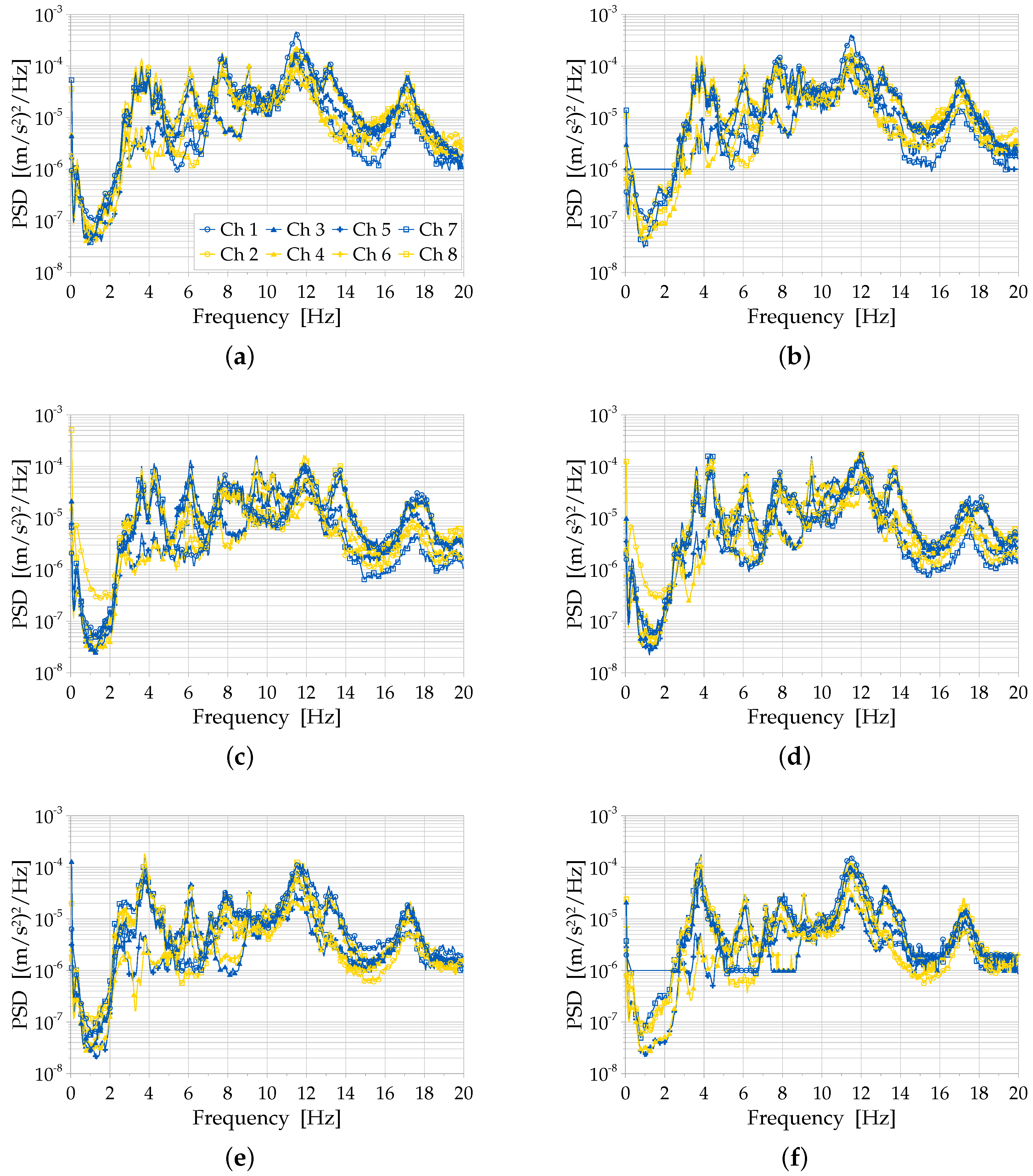
Box 1), it can be stated that the PSDs calculated for each channel practically display zero values above 20 Hz; therefore the analyses and the reported results are extended only up to 20 Hz. All the analyses show that there appear a lot of peaks whose frequencies range from 3 Hz up to 18 Hz. Such presence of several peaks confirms the previous remark on the autocorrelation functions, namely the characteristics of narrow-band signals. Detailed outputs on the obtained results are depicted in
Figure 5 and reported in
Table 2.
In particular, from
Figure 5a, it can be seen that the analyses referred to the upstream of Span 1 show two dominant frequencies, at 7.67 Hz and 11.4 Hz (the peaks of the other frequencies are ten times lower than these two peaks). However, multiple peaks could be detected quite in common for all the channels. Slightly different values are found for the different channels of the same span: this spread around an average value may be due to the combination of the mode shapes, which is dependent on the physical measuring point on the structure; however, 12 (averaged) frequency peaks are detected in at least 4 channels, as reported in
Table 2. The same considerations apply to the results related to the downstream side of Span 1 (PSDs reported in
Figure 5b). In this case, only 8 (averaged) frequency peaks are detected in at least 4 channels (see
Table 2); in particular, the peaks in the range 3–5 Hz diminish, while being more sparse.
The PSDs related to Span 2 show comparable peaks, without any dominant frequency. The peaks in the 3–5 Hz frequency range become even more sparse in this case, only showing up at two frequencies, which turn out at around 3.56 Hz and 4.20 Hz (see
Figure 5c,d).
For Span 3, the PSDs show a trend similar to those for Span 1, except in the 4–5 Hz frequency range, which shows no peak (see
Figure 5e,f).
The comparison of PSDs resulting from the three spans (
Figure 5) allows to outline some main comments. Span 1 displays repeated close peaks at around a 4 Hz frequency, although not remarkably separated, therefore not directly allowing for a unique structural interpretation or identification of the structural modes; in the same frequency range, Span 2 clearly shows repeated peaks, meaningful for possible structural interpretations, namely considering potential mechanical effects of the supporting arches, of the compliance of the piers and of a partial degree of continuity between the spans of the deck, as further discussed in subsequent
Section 6. On the contrary, Span 3 exhibits fewer peaks, possibly related to diverse, perhaps less compliant, structural boundary conditions.
In
Table 2, the main detected frequencies are reported, for peaks identified in at least 4 channels, while frequencies present in all the spans are highlighted in bold font. The frequency around 3.80 Hz is present in Spans 1 and 3, while it seems missing in Span 2, whereas in Span 2 a peak at 4.20 Hz is present and in Span 1 a peak at 7.20 Hz is revealed. In general, the comparison of the PSDs of the channels with the same number on the upstream and downstream sides shows that the dominant frequencies are the same; thus, the behaviour of the spans can be considered rather consistent with respect to the longitudinal axis of the bridge.
A comparison between the here obtained results in terms of deciphered frequency peaks (
Table 2) and the values earlier algorithmically identified by Frequency Domain Decomposition and Stochastic Subspace Identification in [
7] confirms and cross validates both the approaches. In particular, the previously identified modal frequencies on Span 1 in [
7] are here confirmed, with specific reference to the values summarised in
Table 3, which turn out overall common to the three spans, along with secondary peaks described in
Table 2 and possibly helpful for the final structural interpretations, also in view of detailed and distinctive behaviour inspection for each specific span.
Further remarks and structural interpretations of the analysed data are proposed in the subsequent sections, along with the additional refined analyses in
Section 3,
Section 4 and
Section 5, and eventually in
Section 6.
3. Refined Signal Processing Analysis
In order to advance and further investigate the content of the acceleration data, an additional signal processing of a single beat of vibration is performed. At the end of the previous analysis (
Section 2), it was concluded that the frequency contents of the upstream channels are quite similar to that of the downstream channels of each span; thus, the present signal processing refined analysis is performed only on the upstream channels of each span.
The following refined methodological procedure is here considered, in order to further investigate the output data (
Box 2). Through the analysed outcomes of signal processing, some main observations can be derived, specific for each span.
Box 2. Steps of the refined signal processing analysis.
Table 4.
Time properties of the sub-records selected for the refined signal processing analysis outlined in
Box 2.
Table 4.
Time properties of the sub-records selected for the refined signal processing analysis outlined in
Box 2.
| | Span 1 | Span 2 | Span 3 |
|---|
| Sub-Record | 1st | 2nd | 3rd | 1st | 2nd | 3rd | 1st | 2nd | 3rd |
|---|
| Total duration [s] | 8 | 8 | 8 | 10 | 7 | 20 | 12 | 13 | 7 |
| Starting time point [s] | 202 | 464 | 2240 | 1518 | 1714 | 1846 | 1616 | 1628 | 2866 |
| Ending time point [s] | 210 | 472 | 2248 | 1528 | 1721 | 1866 | 1628 | 1641 | 2873 |
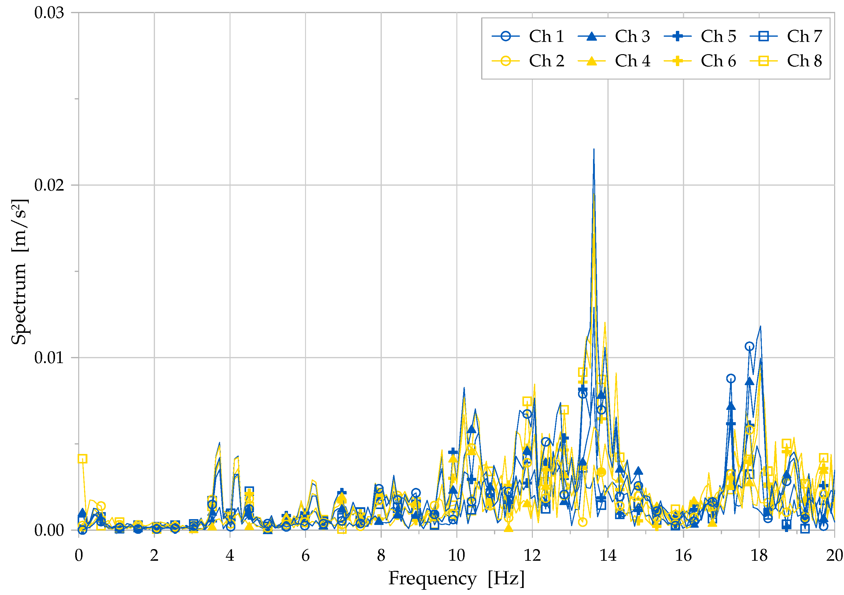
For Span 1, in the first sub-record, Channel 1 exhibits a dominant frequency equal to 11.11 Hz; all the channels display the same dominant frequency, though Channels 2, 6, 7 and 8 are in phase, while 3, 4 and 5 are out of phase. In the second sub-record, Channel 1 shows a dominant frequency equal to 11.49 Hz; all channels show the same dominant frequency, presenting Channels 2, 5, 6 and 7 in phase, while 3, 4 and 8 out of phase; additional peaks appear for several other frequencies in Channels 4, 5, 7 and 8. In the third sub-record, in Channel 1 there appears a dominant frequency equal to 3.25 Hz; Channels 1, 2, 3, 6, 7 and 8 render the same dominant frequency, though Channels 2, 3 and 4 are in phase, while 5, 6, 7 and 8 are out of phase, presenting several peaks in other frequencies for Channels 4 and 5, as shown in the “spectrum” overplot in
Figure 6.
Similar observations can be proposed for Span 2: in the first sub-record, in Channel 1 there are two dominant frequencies equal to 13.49 Hz and 17.80 Hz; Channels 1, 6 and 8 point out to the same dominant frequencies, showing that Channel 6 is in phase, while 8 out of phase; furthermore, Channels 2, 3, 4, 5 and 7 present peaks in a lot of other frequencies (see the “spectrum” over plot in
Figure 7). Analysing the second sub-record, Channel 1 displays a dominant frequency equal to 11.82 Hz; Channels 1, 3, 4, 5, 6 and 8 show the same dominant frequency, having Channels 5 and 6 in phase, while 3, 4 and 8 out of phase; additional frequency peaks are detected on Channels 2 and 7. The third sub-record highlights Channel 1 as a dominant frequency at about 3.39 Hz; Channels 1, 2, 3, 5, 6, 7 and 8 have the same dominant frequency; Channels 2 and 3 are in phase, while 5, 6, 7 and 8 are out of phase; Channel 4 shows peaks in several other frequencies.
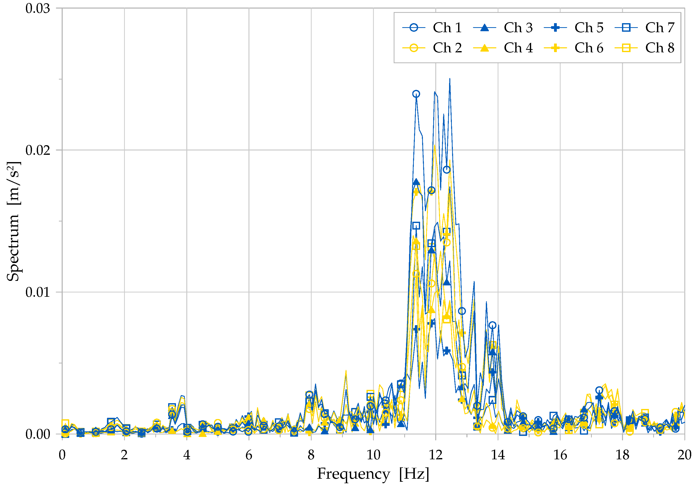
Span 3 allows for further observations of the processed data. In the first sub-record, Channel 1 exhibits four dominant frequencies equal to 8.82 Hz, 9.07 Hz, 11.40 Hz and 11.57 Hz; Channels 1, 2, 7 and 8 mark the same dominant frequencies, being Channels 2, 7 and 8 in phase, while Channels 3, 4, 5 and 6 present very different amplitudes of the peaks. In the second sub-record, in Channel 1 there are three dominant frequencies equal to 2.53 Hz, 11.36 Hz and 11.67 Hz, having the same dominant frequencies in Channels 1 and 8, while the other channels show several additional peaks in other frequencies. The third sub-record highlights, in Channel 1, three dominant frequencies with values equal to 11.28 Hz, 11.86 Hz and 12.99 Hz; the same dominant frequencies are shown in all the channels, however with different peak amplitudes, as reported in the “spectrum” overplot depicted in
Figure 8.
A schematic summary of the dominant frequencies observed during the previous analysis for Channel 1 is reported in
Table 5. From such previous results and observations, it may be concluded that the behaviour of the bridge turns out non-stationary in time, with a response that is quite different at the different measuring points. Furthermore, the presence of positive delays together with negative ones in the cross-correlation functions may be explained by the simultaneous and continuous crossing of the bridge by vehicles going back and forth. Consistently, it should be observed that such loading conditions, as an effect of overlapping vibrations, reduce the effectiveness of the measured data toward interpretation of the current structural behaviour of the bridge, suggesting the adoption of more refined analysis tools, as further inspected next.
4. Wavelet Analysis
In order to come to clarify the interpretation of the current structural behaviour of the bridge, with respect to the observations collected in the previous section and to perform a more refined and detailed analysis of the signals, also in view of setting a general methodological approach, a Wavelet technique is here inspected, to treat the signals, and making part of the methodology. The adoption of such an approach is supported by the outcomes observed in previous
Section 2 and
Section 3, also in the selection of the algorithm features, toward an effective structural interpretation within the proposed methodology of signal processing, specifically for non-stationary response data.
In classical signal processing analysis, the sensor outputs are subjected to signal conditioning to generate functional signal features. The available methodologies can be gathered into three main classes: time-domain methods, frequency-domain methods (both analysed in
Section 2 and
Section 3) and time-frequency domain methods (as here considered by Wavelet analysis). In general terms, the basis functions of Wavelet transform are small waves (namely wavelets) characterised by varying frequency and limited duration, being capable to represent the original signal as a superposition of wavelets. To perform a Wavelet transform, a “mother” or basis wavelet is first selected among different families. The signal is then decomposed into a set of scaled and translated reproductions of the mother wavelet, computing a set of packet coefficients, which represent the correlation between the wavelet and a localised section of the signal. These coefficients can be processed to obtain statistical features, and be used for pattern recognition. Therefore, a Wavelet analysis allows to extract information in the time domain with reference to different frequency bands, with particularly advantageous features in analysing non-stationary signals.
Foundations of Wavelet transformation approaches may be found in the literature (see, e.g., [
18,
38,
39]). In the subsequent paragraphs, a brief summary is recalled. In order to represent general signal function
, a linear combination of wavelet functions is employed (being
t an arbitrary order variable, i.e., time for the present applications). A continuous wavelet transform of the signal can be considered and defined as:
where
is assumed as a wavelet “mother” function (with overbar symbol for complex conjugate), defined on the Lebesgue space of the 2–norm
, having
the set of real numbers. Different mother wavelet types have been extensively evaluated and discussed in [
11], within a specific context of signal denoising, showing that a pertinent choice for handling non-stationary signals shall be that of a Symlet. In the current application, the mother wavelet is implemented through a band–pass Butterworth filter (see, e.g., [
40]), consistently with the Shannon “sinc” wavelet approach [
18].
Each wavelet function needs to satisfy the admissibility condition ruled by the following inequality:
where
is the Fourier transform of wavelet function
.
It turns out that the Fourier transform function
is oscillatory and presents an average value equal to zero. The mother wavelet may present a real- or complex-valued description. For signal decomposition, the wavelet “family” is adopted through scaling and translation operations over the function, such that:
according to the variables and parameters:
t ordering variable, i.e., time;
a scale coefficient;
b translation parameter. The latter parameters assume values in the real set:
, with the additional condition
. Term
, as a scaling factor, guarantees a constant wavelet energy, independently from the scale: namely
. In numerical solutions, a Discrete Wavelet Transform approach can be adopted, avoiding integration steps and an explicit knowledge of the scaling factors and wavelet functions.
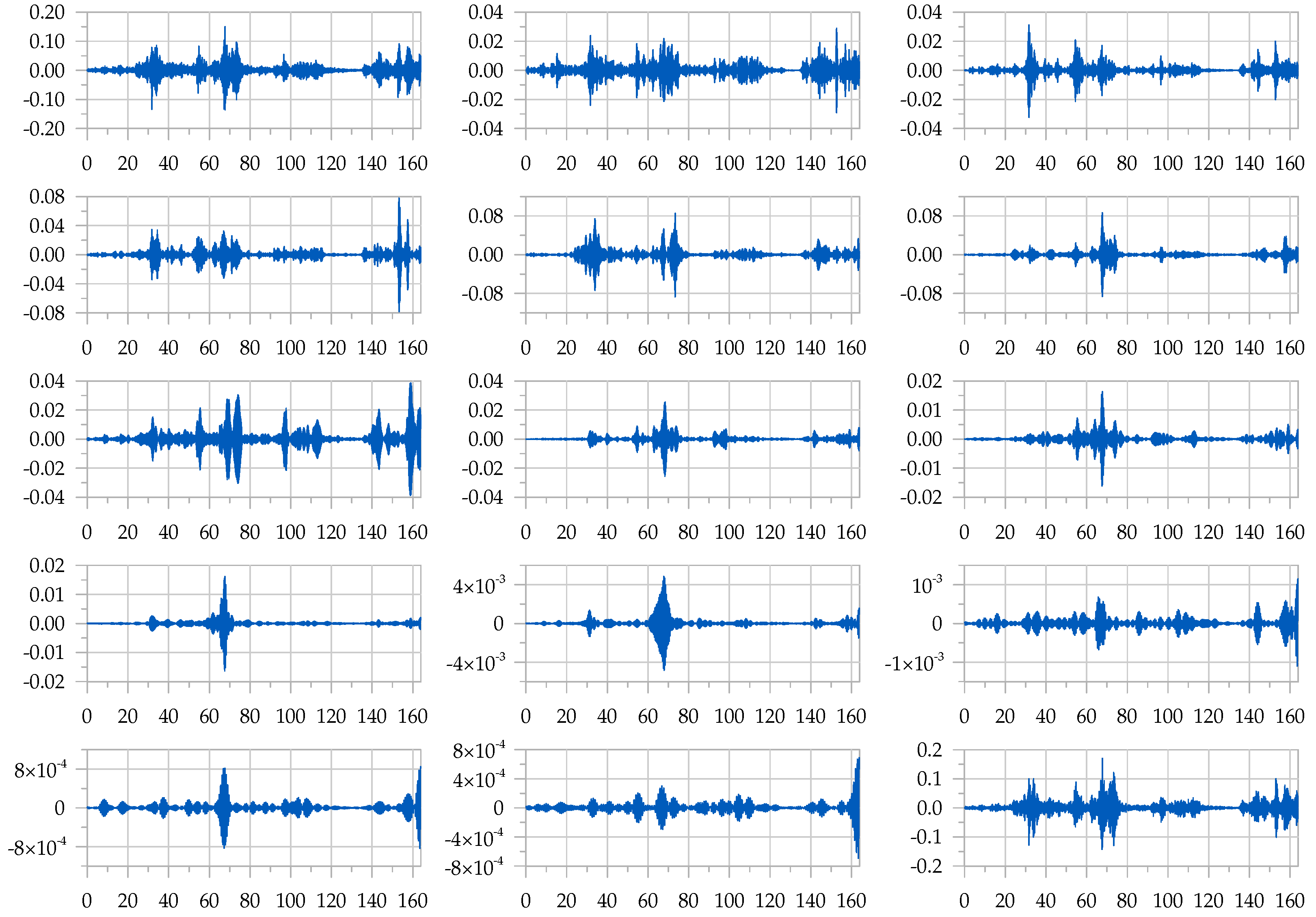
The analysis is here developed through the wavelet procedure by performing a band–pass filtering of the signals, with centre frequencies of the band–pass filter spaced by one-third of an octave in the frequency range from 1 Hz up to 20 Hz. In this way, by observing the position of the frequency components of the signal in the time domain, it is possible to identify the dominant frequencies of the structural response. The dominant wavelet frequency, in each frequency band, is determined in the time domain by evaluating the oscillation period showing the maximum peak. It is worth observing that the analysed signals consider acceleration measurements, thus, generally speaking, the maximum acceleration is occurring at frequencies different from those of the maximum displacement.
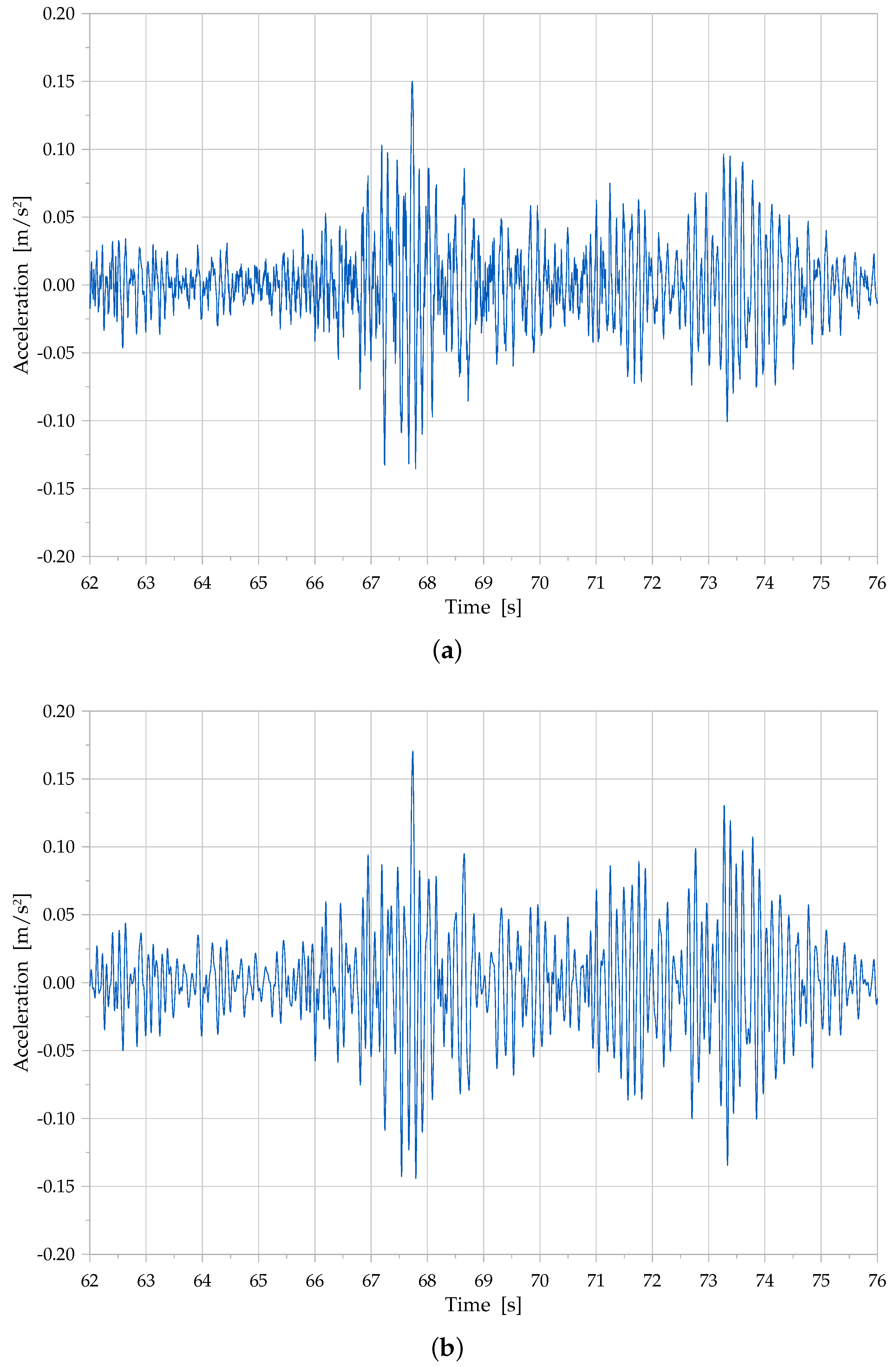
Figure 9 shows the components for each frequency band plotted in the time domain, where the graphs at the top–left and at the bottom–right respectively represent the original record and the reconstructed one, by superposing up all the wavelet components. These last two graphs are newly reported, separately in
Figure 10 (zoom), in order to provide a more detailed representation of the achieved results by the Wavelet analysis; considering that the reconstructed signal is pass–band filtered from 1 Hz up to 20 Hz, the similarity of the two graphs allows to validate the performed analysis. In particular, the effectiveness of the implemented Wavelet methodology is considered according to two main standpoints: an identification approach for the dominant frequencies in the time position, namely considering the advantage of identifying in the time domain the occurrence of the frequencies corresponding to maximum amplitudes; a filtering effect, acting toward either a maximum filtering frequency, i.e., the maximum frequency analysed by the filtering family of wavelets, and a leakage filtering issues, to be considered between each filtering window.
A further remark should be outlined by taking into account that the dominant wavelet frequency is the resultant of the structural response at that specific frequency, determined as the combination of all the modes of the structure, in dependence of the participation coefficient for each mode, in the position of the measuring channel. Specific comments may be proposed about the dominant Wavelet frequencies in the analysis, referring to
Table 6 and
Table 7, and comparing with
Table 2 and
Table 5, showing that dominant Wavelet frequency values should be considered with respect to each specific filtering range, although maximum amplitude values (bold font in
Table 6 and
Table 7) may come to represent true structural dominant frequencies or interaction of them, namely frequencies associated to combinations of the structural modes of the bridge. It is worth observing that the latter case may require further developments, to properly distinguish the combined components and to assess each specific behaviour of the infrastructure.
Table 6 and
Table 7 show the deciphered dominating wavelet frequencies, as above defined, from the upstream and downstream sides, respectively, of Span 2 (mid-span on pillars within the river).
The analysed record is lasting 163.84 s for both the analyses and the starting point is at time 2780 s, for the upstream side, and at time 135 s, for the downstream side, from the beginning of the record on the span. Both tables are reporting the frequency and the corresponding maximum acceleration and harmonic displacement (i.e., computed from the acceleration under the hypothesis of a sinusoidal wave signal) for each frequency band; it has to be noted that the maximum acceleration is occurring at different times, for each frequency band. This last remark also holds true for different channels.
From
Table 6 and
Table 7, it appears that the outcomes from the two sides manifest in different ways: the positions with the same number display different dominant wavelet frequencies. A lack of symmetry (with respect to the mid-longitudinal plane of the bridge) in the current structural behaviour of the bridge, as highlighted by this Wavelet signal analysis, though originally not conceived, would require a further deepening and understanding, as proposed in
Section 6, for interpreting a potential non-linear or damaging behaviour of the bridge, in the present conditions.
In order to further investigate the sources of apparent non-linearity in the response data of the bridge and to propose an alternative and promising processing methodology, the experimental acceleration data are now newly reconsidered in the subsequent section, by employing an ARMA model approach.
5. ARMA Model Analysis
In the current section, further analyses are proposed, exploiting the tool of AutoRegressive Moving Average (ARMA) models, with the goal of achieving an improved understanding of the non-stationary monitoring vibration data, toward investigating the current structural behaviour of the bridge.
A classical theoretical reference on the methodology may be found, e.g., in [
30,
41], while a brief recall of the main features is provided in the following. The ARMA model theory is based on the study of models suitable to produce time series of collected data, starting from a white noise input. Such a model is considered to be a “black–box model” with the following relevant characteristics: quick setup of the model; easy way to build a model for very complex systems; non-required physical knowledge of the system; high-quality precision of the developed model, possibly tuned by a given degree of approximation. On the contrary, a “white–box model” would provide results easier to be interpreted, thanks to the knowledge of the content of the model itself and to a higher confidence in managing the numerical tools.
It has to be noted that, in many case studies, the white noise input is not known, like in the current case of operational excitation input, due to ambient conditions and traffic loading traversing the road bridge.
Considering the ARMA models as the most precise models for linear, time-invariant dynamic systems, the output of a black–box system may be written as:
where the terms correspond to:
, input signal in the time domain,
, unmeasured noise that is transformed by the system (noise going through the system and contributing to the output);
q delay operator,
;
,
;
, frequency response function of the system;
, impulse response function of the system.
Generally speaking, the delay operator may be written as:
where for
,
, being
the system frequency response function.
The noise function may be expressed as:
being
white noise, with
root mean square value, and being
a filter function of the white noise. It is worth noting that a Gaussian noise (i.e., a noise with a Gaussian amplitude distribution) does not necessarily refer to white noise, yet neither property implies the other. While Gaussianity refers to the probability distribution with respect to the instantaneous value, the term “white” refers to the way the signal power is distributed (i.e., independently) among the frequencies. Therefore, the white noise displays a constant value of the Power Spectral Density in the frequency domain; nevertheless, it can show any kind of continuous probability distribution.
The output of the system may be written as:
Generally speaking, the system equation may be rewritten, considering diverse updates of the model; by equations, referring respectively to an ARX model (AutoRegressive eXogeneous model), an ARMAX model (AutoRegressive Moving Average eXogeneous model), a classical ARMA model (AutoRegressive Moving Average model) or an AR model (AutoRegressive model):
In the present work, a Matlab environment [
42] is adopted for delivering a self-implementation of the numerical analyses with the ARMA models, for the analysis of a vector
y which represents the output of the system and for the analysis of a matrix which represents the
n simultaneous outputs of the system. Thereby, set parameter
as the degree of polynomium:
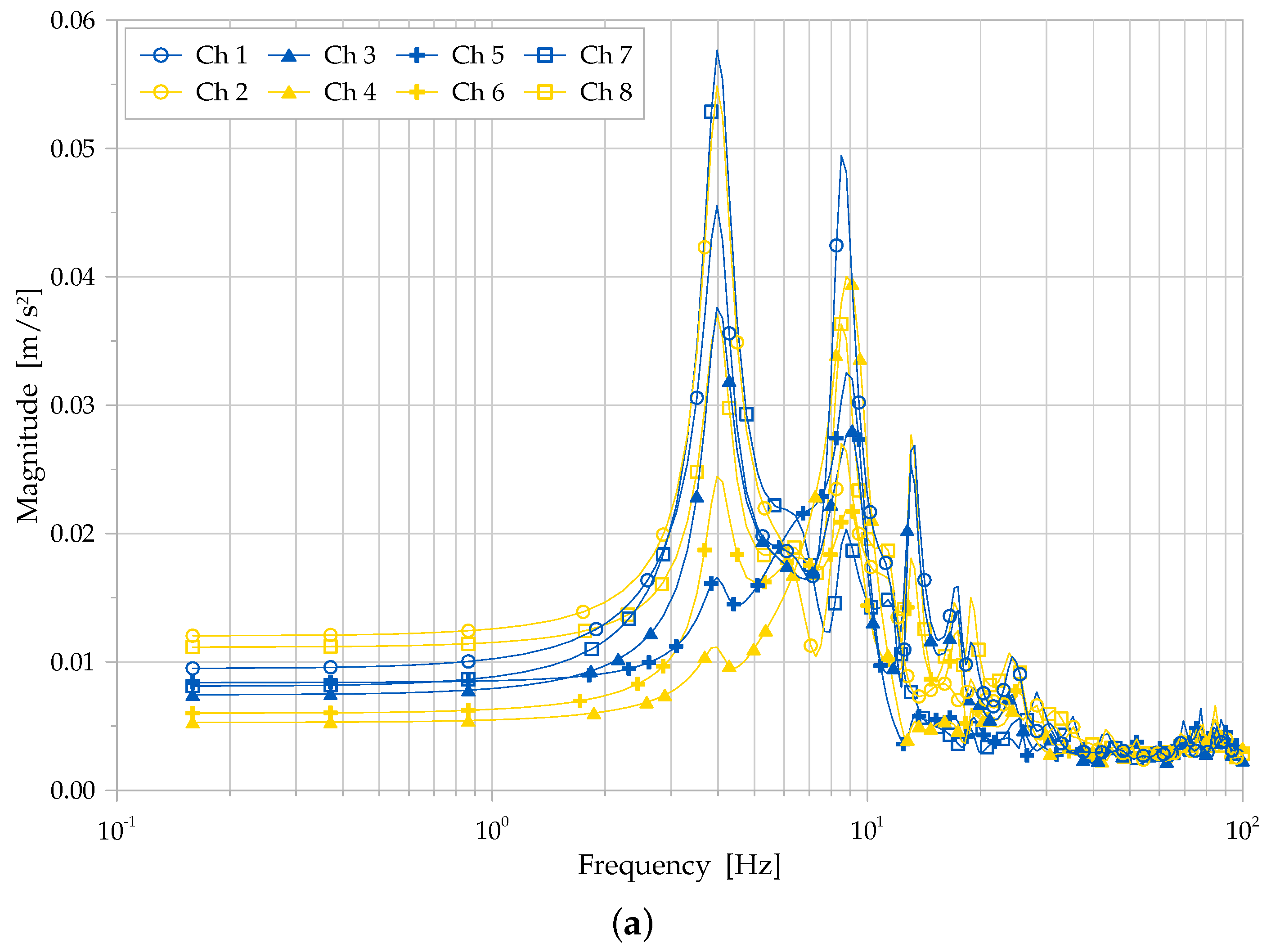
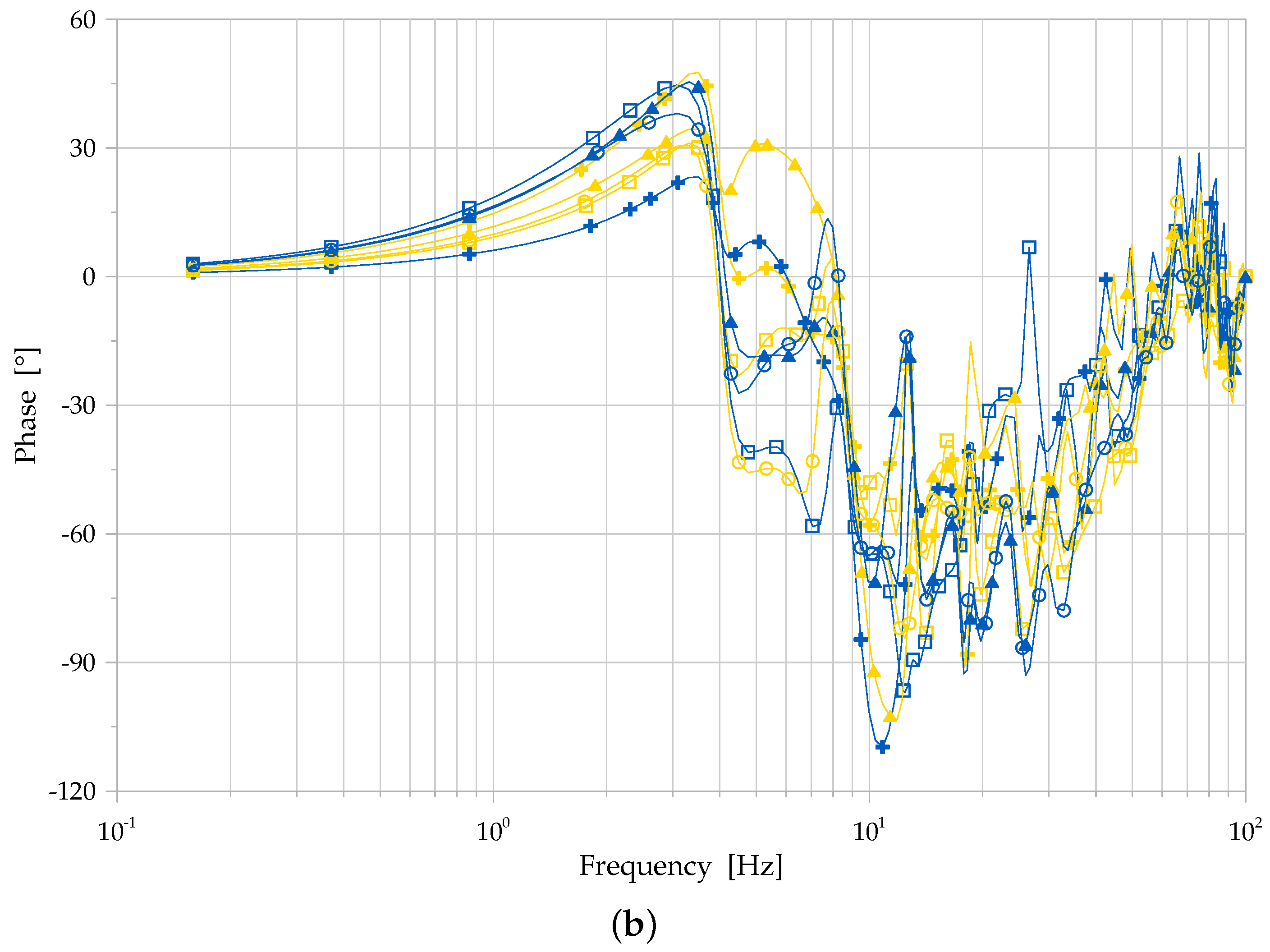
In order to describe the outputs of an ARMA model analysis, knowing that the frequency response of a linear dynamic model describes how the model reacts to harmonic inputs, the Frequency Response Function (FRF) is often depicted by two types of plot: one showing the amplitude change of the output and one displaying the phase shift, as a function of excitation frequency, namely a so-called Bode plot.
The described models are employed for the case study on the Brivio bridge, referring to Span 2, upstream side, with four different evaluations of the model transfer function, markedly in terms of the extracted Frequency Response Function.
- (A)
Investigation by matrix analysis (eight channels) of a time window equal to the first 72 s of the whole record
- (B)
Investigation by matrix analysis (eight channels) of a time window equal to the first 100 s of the whole record.
- (C)
Investigation by matrix analysis (eight channels) of a time window equal to the first 200 s of the whole record.
- (D)
Investigation by matrix analysis (eight channels) of a time window equal to 72 s, at starting time 1625 s of the whole record.
The specific results achieved out of the present ARMA implementation are synoptically reported in
Figure 11, as the most representative and typical Bode plots (ARMA model (B), whole set of eight channels), in order to display the magnitude and phase diagrams, as characteristic features of the extracted FRF, as evaluated by the ARMA approach. The results depicted in the magnitude diagram of the Bode plot of the FRF (
Figure 11a) highlight some main peaks in the response function, consistent with the data in
Table 2,
Table 3 and
Table 5. In addition,
Figure 11b displays the phase shift on the Bode plot for the FRF, where it may be observed, in particular, a marked negative phase shift for frequencies higher than 10 Hz, suggesting a filtering or damping effect above that frequency threshold.
From the results of the ARMA processing of the acquired data, the following main remarks hold. The suspected non-stationarity of the recorded data looks confirmed and the resulting FRFs turn out strongly dependent upon both time location and length of the processed record. Therefore, considering the analysis procedure, the extent of the sampling window should generally be selected for the model, possibly in consideration of the excitation loading conditions and the sought structural properties. Similarly, it turns out necessary to set a suitable criterion to select the type of the sub-records: either high peak values, high RMS values or local stationarity. Moreover, it is worth observing that a time compression procedure appears to be helpful to the aim of removing the zero–signal content parts, confirming, on one side, the need for future developments and further deepening and, on the other side, the promising features of ARMA model applications toward structural identification and interpretation.
6. Summary of Signal Processing Methodology and First Structural Interpretations
With respect to the contents described in previous
Section 2,
Section 3,
Section 4 and
Section 5, focused on the methods, procedures, outcomes and specific observations regarding the adopted general methodology of signal processing (resumed in
Box 3), the further main goal of the present section is to propose, as supported by the analysis results, some first interpretations on the current structural behaviour of the Brivio bridge. In particular, and with specific reference to previous analyses presented in [
7], the investigation is here developed considering additional structural features of the Brivio bridge, namely the possible influence of the parabolic arches on the vibration response of the whole structure and the deck, and the possible sources of non-linear phenomena in the monitored data, with a final resuming assessment on the dominant frequencies of the bridge infrastructure.
Box 3. General frame of the devised methodology of signal processing.
First signal processing analysis (as outlined in
Box 1)
Refined signal processing analysis (as outlined in
Box 2).
Wavelet analysis.
ARMA model analysis.
6.1. Influence of the Arches
With reference to the earlier observed results in [
7], it is here meant to attempt to address the following two main quests:
what is the meaning of the two first close natural frequencies of the bridge, displaying the same mode shape (referring to readouts at the deck only);
why the first two-mode shapes of the deck present a nodal point and the mode shape of the immediately higher frequency does not show a node symmetry.
Generally speaking, looking at the deck of a span as a beam or as a rectangular plate, it is expected that the first natural frequency shall present a mode shape with no nodes, making therefore of interest to understand why the bridge looks to present the behaviour described above. Taking into account that during the recording of ambient vibrations there were no measuring positions on the arches of the bridge (namely just sensors positioned on the deck), it can be expected that the behaviour of the whole structure could not completely be deciphered. In the following, an attempt is made to evaluate whether the supporting arches may display a structural dynamic behaviour that could influence the overall dynamic response of the spans of the bridge.
To evaluate the behaviour of the supporting arches of the bridge, the first reference is made to [
43,
44,
45]. Circular arches are therein considered for simplicity; nevertheless, the study of the behaviour of circular arches may first help to answer the above two basic questions, with which it is dealt here. Further refinements and observations may be derived, in future research, considering more detailed analyses (see, e.g., [
46,
47]), possibly coupled with additional numerical and model updating approaches, beyond those already produced in [
7].
First of all, the behaviour of simply supported arches with a complete opening angle is considered, which can be summarized as follows:
the mode shapes may be symmetrical or anti-symmetrical and their natural frequencies depend upon the slenderness ratio of the arch, defined as the ratio between the span of the arch and the radius of gyration of the cross-section of the arch;
the first symmetrical mode shape shows two nodes, one on each mid-span, while the anti-symmetrical mode exhibits one node in the centre of the arch;
in any case, the anti-symmetrical mode shape appears to be characterised by a natural frequency always lower than that of the symmetrical one.
In the following, the comparison of the dynamic behaviour of simply supported and fixed ended arches is considered, whose main conclusions may be stated as follows:
the mode shapes may be symmetrical or anti-symmetrical and their natural frequencies depend upon the slenderness ratio of the arch, irrespectively of the boundary conditions;
the first symmetrical mode shape has two nodes, one on each mid-span, and the anti-symmetrical one has one node in the centre of the arch, irrespectively of the boundary conditions;
in any case, it appears that the anti-symmetrical shape displays a natural frequency always lower than that of the symmetrical one, irrespectively of the boundary conditions and of the opening angle.
Observing that the supporting arches of the Brivio bridge are endowed with a parabolic shape and taking into account that the span of the arch is 42.8 m and the height of the arch is 8 m, the corresponding equation of the parabolic arch, referenced at mid-span, can be given as [m]: .
As a consequence, the opening arch angle results in about 106°. Such arch configuration, for the present considerations, may be approximated by a circular arch with a radius of 35.74 m and, with a reasonable engineering approximation, the conclusions of the previous paragraph may be applied to such a structural scheme as follows:
the first natural frequency of the arch shows an anti-symmetric mode shape with a node in the centre of the span;
the dynamic shape of the first mode of the arch shall influence the deformation of the deck of the bridge, which will respond with a node at mid-span.
It should further be observed that a small difference between the first natural frequencies of the upstream and downstream arches may also be a reason for the two close frequencies detected in the dynamic response as measured at the deck of the bridge.
6.2. Non-Linear Behaviour Conjecture
Concerning the hypothesis and interpretation of the linearity or non-linearity of the structural behaviour of the bridge, in order to improve the understanding of the vibration response of the bridge, the following observations may be outlined:
the distribution of the instantaneous values of response is strongly different from that of a Gaussian distribution;
the distribution of the positive and negative peaks fits quite well a Weibull distribution, with parameter at about 1.1, while it does not fit at all a Rayleigh distribution, as a confirmation that the distribution of the instantaneous values is not normal;
provided the knowledge that the response of a linear system is a Gaussian process, if the excitation is a Gaussian process and the linear operations will tend to suppress any deviations from the Gaussian form that may exist, if the vibration due to stationary traffic on a bridge may be considered as a Gaussian process, the response of a bridge with a linear behaviour should be a Gaussian process;
on the contrary, the response of a non-linear system is not a Gaussian process even if the excitation is a Gaussian process, suggesting the conclusion that the behaviour of the Brivio bridge seems to be a non-linear one, as observed with a Gaussian process input and a non-Gaussian recorded response process.
A confirmation of the potential non-linearity of the structural behaviour of the bridge could be assessed by evaluating the presence of harmonic distortions in the response of the bridge to harmonic excitation. However, this kind of analysis was not pursued so far in the study of the Brivio bridge, while the excitation due to ambient vibration generated by road traffic turns out to correspond to a multi-frequency excitation. Possible future performance of forced vibration tests with a harmonic excitation may be considered, to provide support in further assessing the possible linearity vs. non-linearity of the recorded response behaviour of the bridge.
6.3. Structural Frequencies of the Bridge
With reference to the observations in the previous sections and specific paragraphs and, particularly, considering the output data gathered in
Table 2,
Table 3,
Table 5,
Table 6 and
Table 7 and
Figure 5, it is possible to identify some effects of deviation from the originally conceived structural behaviour of the bridge, namely differences between the response of the spans and between the upstream and downstream sides. A numerical comparison of the collected peak frequencies of the bridge (see
Table 2 and
Table 3) with the previously identified data in [
7] cross-validates the employed methodologies and suggests, in future research, the adoption of complete model updating procedures for the study of the whole bridge structure, in view of achieving a global and effective process.
Focusing on the structural interpretation of such phenomena, i.e., without specific consideration for the traffic loading conditions, some issues shall be identified:
compliance of the boundary conditions, i.e., bridge abutments and piers, possibly affected by deterioration or scour effect within the river bed (see, e.g., [
48]);
stiffening effect and implication of the supporting parabolic arches, as firstly commented in the previous paragraphs;
possible partial degree of continuity of the deck beam across the simply supported spans;
apparent non-linearity in the structural response, possibly related to damping effects and deterioration of the mechanical constitutive properties of the underlying materials (see, e.g., [
49,
50]).
As an advancement in the investigation of the current structural behaviour of the Brivio bridge, the earlier results presented in [
7], the present analysis on the three spans allows for further global observations, as here consistently commented, suggesting a reliable and refined SHM procedure to be developed for the bridge, both at a local, i.e., material and constraints, level and at a global structural level, possibly in view also of evaluating potential future intervention and conservation scenarios, for the over hundred-year old structure.
7. Conclusions
The main aim of a systematic signal processing data analysis, as developed in this paper for the case study on the Brivio bridge, was that to produce a blind test on a comprehensive methodological procedure, with the further target to identify reliable structural features, such as the dominant frequencies of the structure, and to provide structural interpretations, like for the influences of specific functioning parts (e.g., arches, deck, bearings and boundary conditions) and for potential manifestations of global non-linear behaviour. This is extracted out of (non-stationary) response signals, recorded just on the bridge deck by standard wired accelerometers, over an earlier three-day spring experimental campaign, overall concerning all the three spans of the bridge.
The following general remarks and issues on the whole signal processing methodology and analysis may be drawn.
The quality of the recorded signals looks suitable for quite refined analyses (see, for instance, source and reconstructed signals by the Wavelet analysis,
Section 4 and
Figure 10). The adopted recordings may be affected by different ambient conditions, for instance, temperature (see, e.g., [
51]). However, an analysis of such types of effects appears to be out of the scope of the present investigation, though they may be considered for further experimental campaigns, as pointed out below. On the other hand, it is believed that the present analysis allows us to outline a number of fundamental features (such as non-stationarity of the response data, the influence of the arches on the mode shapes, non-linear behaviour, dominant frequencies), of the response signals and of the source infrastructure, which already provides a rather general and fundamental understanding, toward final structural interpretation.
A first preliminary analysis was performed on the full record of each of the eight measuring channel signals on both the upstream and downstream sides of all the three spans of the bridge, by determining the maximum, minimum and RMS values and by calculating their statistical distributions; moreover, correlation and spectral analysis were performed.
The outcomes of the above described preliminary analysis were summarized in
Table 2, as far as the dominant frequencies from all the signals; moreover, although the general characteristics of the signals turn out the same, for each channel and among the different channels, the signals of all the measuring positions result non-stationary, neither along the full record, neither on reduced duration records; for this reason, it was envisaged to apply special techniques for the statistical analysis of non-stationary data, among others a Wavelet analysis and an ARMA model.
As a first refinement of the analysis, three sub-records with a limited duration and with a high level of response were chosen, for each side and for each span. For each sub-record, the autocorrelation function and the “spectrum” (Fourier amplitude) were calculated and the crosscorrelation function between Channel 1 and each one of the other channels was determined. From this refined analysis, it may be concluded that the response of the bridge looks non-stationary in time and that the structural response presents different characteristics, as deciphered at the different measuring points.
For a more refined and detailed analysis of the signals, a Wavelet technique was further applied to the same two channels on each side of the middle span of the bridge. From
Table 6 and
Table 7, it appears that the upstream side and downstream side behave differently, as prompted by diverse dominant wavelet frequencies displayed by corresponding positions.
An additional refined analysis has been developed for some sub-records from Span 2 by ARMA models, confirming some main peak frequency values of the bridge (see
Table 2,
Table 3 and
Table 5). However, consistently, this stage of the study highlighted a non-stationarity character of the recorded data, as displayed by the Frequency Response Functions, requiring future further deepening, both in the signal sub-record selection and in the ARMA model methodological approach.
Further remarks may be drawn regarding a first structural interpretation of the current behaviour of the bridge, from the developed comprehensive signal processing analysis as in the followings.
The distributions of the instantaneous values and of the positive and negative peaks do not respectively fit a Gaussian distribution and a Rayleigh distribution; thus, the signals look like non-stationary, random normally distributed signals. A possible motivation for such features may be located by assuming that the bridge is not behaving as a linear structural system or that the traffic excitation is a stationary stochastic process having a probability distribution different from the normal one.
Not having a controlled input excitation onto the bridge, the AR (AutoRegressive) model was considered suitable for the study, even if, as here above mentioned, the excitation could not be considered to be a stationary stochastic process; the ARMA data processing confirmed the non-stationarity of the data, showing in the resulting FRF a strong dependence upon both time location of the processed record and length of the record.
The classical treatment of the dynamic behaviour of the arches may help to understand the presence of the first mode shape of the bridge with a node in the middle of each span, likely implied by the first natural frequency of the arch with an anti-symmetric mode shape, with a node in the centre of the arch itself; thus, the dynamic shape of the first model of the arch may influence the deformation of the deck of the bridge itself.
The analysis reasonably stays at the first, mainly qualitative, deductions that can be extracted from the acquired data, as deciphered through the present analysis. On the other hand, the elaborations on the estimation of the structural frequencies, do already provide quantitative measures of the current structural properties.
Mainly, in terms of salient aims and achievements of the study, the present contribution:
- (a)
forms a specific SHM case study, on a bridge of a peculiar infrastructural and historical value;
- (b)
assembles a general, replicable methodological procedure for systematic signal processing analysis; in that, standard techniques are employed (although ex-novo implemented and adapted to the specific case) and value should be recognized in the assembly of the whole, as a general methodology for data treatment, also for non-stationary response signals (see
Box 1,
Box 2,
Box 3), in that realm, possibly to be extrapolated to other similar case studies;
- (c)
runs it and delivers comprehensive results, with selected illustrative samples reported in the paper, and corresponding outcomes;
- (d)
seeks a final deciphering of the outcomes, toward interpretation of structural features and response characteristics of the bridge at hand.
The innovative contributions discussed by the case study investigation on the Brivio bridge highlighted several remarks both on methodological procedures and on first structural interpretations. In particular, it is worth observing that the effectiveness of consistent signal processing approaches as here advised (see
Box 1,
Box 2,
Box 3 in the paper, which shall have set a general signal processing methodology) is definitely confirmed, toward the final structural identification and interpretation.
Moreover, the global complete analysis of the responses concerning the structure, combined with the adoption of more refined signal processing tools, such as Wavelet analysis and ARMA modelling, allows for a further and more specific understanding of the current structural behaviour of the bridge. Therefore, the analysed results confirm, from a structural standpoint, the suggested need for setting an effective and reliable Structural Health Monitoring platform, possibly supporting the historical and fundamental infrastructural role of the Brivio bridge, also in view of restoration and conservation scenarios.
Therefore, the proposed contribution displays a functional assembly of existing techniques, in view of forming a feasible, self-implemented, general platform for signal processing analysis, with scopes of SHM at the Civil Engineering scale, with specific reference to infrastructure applications, as per the structural assessment of the considered historic bridge. It may serve as a guideline to process and interpret response signals, also when endowed with a non-stationary character systematically and effectively.
In terms of final deciphering of the natural frequencies of the structure, and more generally of a complete modal dynamics identification, after the present signal processing analysis, focused on the data treatment and with a first assessment of the dominant frequencies of the structure, a further detailed modal identification could be explored by inspecting the adoption of specific dedicated techniques, to be applied to the signal data, as here discussed and evaluated (in particular, on the full-time record or in sub-records), as per the regular and refined analyses in
Section 2 and
Section 3, or possibly before and/or after the Wavelet analysis or the ARMA model application, i.e., either on the source and/or the reconstructed signal or on “black–box” system modelled responses. This may be targeted to achieve quantitative estimations also of the mode shapes and, as well, of the mode damping ratios of the structure. Specifically, within the Frequency Domain, a “refined Frequency Domain Decomposition” (rFDD) technique, as methodologically outlined in trilogy [
52,
53,
54], could be employed, as systematically applied in [
55,
56,
57] (in a specific challenging context of non-stationary response signals, as that of seismic engineering), as well as in conjunction and/or comparison with identification strategies in the time domain, such as improved Data–Driven Stochastic Subspace Identification (SSI–DATA), as explored in [
58,
59]. This subsequent potential study, devoted to further investigate the implications of the present comprehensive signal processing analysis, in terms of additional and final interpretation of the present dynamic structural features of the bridge, may be considered for further, complementary work.
The current stage of analysis, and interpretation, provides the first run of inspection, based on data recordings that have been acquired. The present study could serve as a basis for possible further actions, in view of gaining an increased understanding of the structure at hand. Concerning further acquisition and processing, as future developments, it may be concluded that some further tests and additional measurement points provided on the arches of the bridge should help in achieving a wider experimental description of its dynamic behaviour. Additionally, some differential displacement transducers on the hangers of the bridge or on specific, possibly damaged, locations could be suitable, to enquire the behaviour of the arches and the implications on the response of the deck, being the two behaviours truly structurally coupled. Future investigation on ambient factor-induced responses would as well be possible, if the scheduling of additional measurements could be carried out, in different seasons and times, to additionally inspect issues of environmental effects, such as temperature, sun exposition, humidity, etc. (see, e.g., a wavelet-based analysis, self-coherent with that here inspected in
Section 4, recently developed in [
51], for thermal response separation of bridges, within long-term monitoring). Further, a broader application of the advanced analysis techniques, as here pointed out, like Wavelet and ARMA models, could also be advisable, with the aim to achieve a deeper study on the applicability of signal processing toward reaching a definite, consistent structural interpretation.


