Accurate Simulation of Neutrons in Less Than One Minute Pt. 2: Sandman—GPU-Accelerated Adjoint Monte-Carlo Sampled Acceptance Diagrams


European Spallation Source ERIC, Box 176, 221 00 Lund, Sweden
Quantum Beam Sci. 2020, 4(2), 24; https://0-doi-org.brum.beds.ac.uk/10.3390/qubs4020024
Submission received: 20 May 2020
/
Revised: 9 June 2020
/
Accepted: 12 June 2020
/
Published: 16 June 2020
(This article belongs to the Special Issue New Trends in Neutron Instrumentation)
Abstract
:A computational method in the modelling of neutron beams is described that blends neutron acceptance diagrams, GPU-based Monte-Carlo sampling, and a Bayesian approach to efficiency. The resulting code reaches orders of magnitude improvement in performance relative to existing methods. For example, data rates similar to world-leading, real instruments can be achieved on a 2017 laptop, generating neutrons per second at the sample position of a high-resolution small angle scattering instrument. The method is benchmarked, and is shown to be in agreement with previous work. Finally, the method is demonstrated on a mature instrument design, where a sub-second turnaround in an interactive simulation process allows the rapid exploration of a wide range of options. This results in a doubling of the design performance, at the same time as reducing the hardware cost by 40%.
1. Introduction
Neutron scattering facilities such as the European Spallation Source (ESS) currently under construction in Lund, Sweden, and the world-leading Institut Laue Langevin (ILL) in Grenoble, France, rely increasingly upon beam simulations to steer the evolution of the design of their instruments. The credibility of instrument conceptual design is now largely driven by Monte-Carlo simulation in preference to the more traditional approach of using analytical derivations. Such a change already happened in other fields—such as high energy and nuclear physics—due to the increased complexity of the respective scientific problems. Indeed, part of the reason in neutron scattering is likely to be the use of more complex instrument geometries, as will be touched upon in later sections of this paper.
There exist several software packages for building Monte-Carlo simulations of neutron beams, the most popular being McSTAS [1], SimRes [2], and VitESS [3]. McSTAS has the widest user base, and requires the user to write a modified version of C. VitESS has a design philosophy around GUI-based, modular, pre-compiled code running sequentially via pipes. SimRes allows easy switching between bi-directional simulation options, either forwards or the adjoint Monte-Carlo method in reverse.
Neutron guide simulations can be a very time consuming activity. A large fraction of the computing resource allocation at ESS was not just for neutronics jobs but also McStas simulations of guides.
In this paper, a new software methodology and tool for the design of neutron guides is described, called “Sandman”. It is currently available on GitHub [4], and offers significant computing speed improvements over the existing codes. It is written in C++, and is provided as a library. Instrument descriptions are written as a single instance of a class, and then a sequence of geometrical functions from that class. This is compiled and linked to the library.
There are three significant differences between Sandman and existing codes, though naturally each of these have a solid grounding in computational physics.
Firstly, Sandman works directly on 2-D phase space maps, called acceptance diagrams (see, for example, Reference [5]). These are maps of beam divergence angle and position y that are transmitted by each component. By manipulating these maps, one can accurately define the transmission region of the beam from one optical module to the next. The principle was computationally automated for monochromatic beams in a previous technique called neutron acceptance diagram shading (NADS) [6]. It provided a significant performance gain for the simulation of high resolution instruments, which would normally take several hours on large computing clusters using 3D Monte-Carlo approaches.
The main drawback with acceptance diagram shading is that it is monochromatic. A poly-chromatic neutron beam, such as produced by spallation sources, requires multiple passes or an assumed wavelength integral range that is small (≲15%). For example, a mechanical velocity selector, monochromator, or narrow bandwidth chopper instrument would require normalisation simply by multiplying by the width of the wavelength band. This approximation breaks down for poly-chromatic beams.
The solution for wide bandwidth poly-chromatic simulations is to marry the acceptance diagram shading technique with a Monte-Carlo sampling approach. It is important to note that this results in quite a different code compared to existing 3D Monte-Carlo approaches. The acceptance diagram shading method is two dimensional, and intrinsically faster than 3D ray tracing for an identical optical system. As will be shown later in this article, there is no planar intersection to solve. The fundamental requirement in the 2D method is that the horizontal and vertical phase space maps are independent, as one obtains from neutron guides with quadrilateral cross sections. Octagonal neutron guides or those with mirrors that are similarly inclined in a diagonal sense, so as to mix the horizontal and vertical phase space, cannot be modelled at present using NADS or Sandman, though the use case for such guides is quite narrow. Until this phase space mixing is implemented, second order effects such as rotational misalignment or multiple scattering cannot be done internally and would rely on external software.
The second major feature of the code is the adjoint method, reverse tracing, which is a long-time optional feature of SimRes [2]. Adjoint Monte-Carlo was formulated at an early stage in computer simulations, as a variance reduction method to deal with neutron and photon shielding issues [7], and has been demonstrated in high energy physics [8]. It also has precedence in computer graphics ray tracing for decades, enabling CGI effects in movies, interactive 3D simulations and computer games. One would not trace photons from a light source in all possible directions and hope that the ray eventually intersects the camera location. Similarly, in the design of a neutron optical system, it will be shown in Section 2.1 why one should start at the sample end of the guide. Sandman is written in such a way to only compute the adjoint physical model. The adjoint method can be more problematic, particularly in the case of shielding and high energy work where particle interactions and secondary particles are created. However, in the current application of simple, non-interacting particle beams, these additional complications are not present.
Thirdly, Sandman is not designed to run on the CPU, like traditional software, nor is it a hybrid code that detects available hardware and deploys itself to the most efficient devices. Instead, it is written purely for the graphics card (GPU) using the Cuda API. This paper represents a second (and successful!) attempt to produce pure GPU neutron beam simulations. The first attempt failed in 2008–2010, in the sense that the CPU code was still faster, for a number of reasons. Cuda was a very new API at the time, and the development was in very early stages. The GPU memory transfer bottleneck, and the available memory, were major code design issues: one had to prepare the memory, process the data, and receive the output data quicker than simply doing the computation on the CPU. The direct computational treatment of acceptance diagrams was also a fairly new idea. The developments that enabled a successful project this time, starting in 2018, are a combination of easy access to good pseudo-random number generators on the GPU; an increasingly large memory bandwidth driven by the hardware needs of the 3D game industry; multiple GB of GPU memory being available; and mature, parallel methods to reduce large arrays of data.
The speed of this code brings great utility. Sandman offers a neutron guide designer the possibility of simulating a neutron guide with performance matching that of many real-world instruments in real-time, namely ∼ neutrons per second on the sample. From the perspective of the guide designer, running a white beam simulation is essentially instantaneous.
2. Description of the Method
2.1. Reverse Tracing
Sandman is an adjoint method, modelling the neutron beam in reverse, starting at the sample end of the guide. To see why this is effective, one must first consider the neutron transport system as a black box with a transmission efficiency T in the forwards direction, and in the reverse direction.
The probability that a neutron trajectory passes successfully from the source to the sample is a conditional probability , where is the probability that the neutron emerges from the system and reaches the sample, and is the probability that a neutron successfully enters the guide system from the moderator. Thus we see that T, the forwards transmission efficiency, is the conditional probability that a neutron hits the sample, assuming it enters the guide.
Existing Monte-Carlo codes generate trajectories already by pre-selecting the edges of phase space so that the generated trajectories have . The problem is that, as the resolution of the instrumentation increases, T becomes increasingly small. Neutron fluxes at the guide entrance could be – n/cm/s, decreasing to on-sample fluxes of n/cm/s. Calculating T in the optimisation of a high-resolution small angle scattering instrument requires many CPU-hours of computing time [6].
Now, if we consider the adjoint problem, in reverse —this is the conditional probability that the neutron trajectory intersects the moderator, assuming that the trajectory intersects the sample position. If we only generate neutron trajectories at the sample such that , then accurately simulating by computing backwards is significantly faster than the equivalent simulation of T by computing forwards.
To see why this is so, we must only consider Bayes’ theorem:
Or equivalently, . The moderator illumination is designed to be as efficient as possible, that is, maximising , whereas the instrument Q resolution is inversely proportional to terms depending on , so . T also depends on the beam conditioning in general, which prepares the divergence and wavelength ranges to a minimum tolerable value that define the Q (=) and E resolution, so . T is often very small, typically with x in the range 3–6, and is therefore very close to 1. Hence, there is a difference that is several orders of magnitude between and T in computing time. All that remains afterwards is to multiply by the moderator brightness, as usual, and normalise the initial phase space to the much smaller area and solid angle factors of the sample to guide exit rather than the moderator-guide entrance phase space as one would for T. It is a useful exercise for the reader to verify for themselves that the two calculation directions produce an identical numerical result for the instrument performance, but it is an intuitive result. After all, the classical geometrical equations for non-interacting particles are independent on the direction of time.
2.2. Neutron Trajectory Calculation Method
2.2.1. GPU Software Development
Graphics accelerator cards were originally designed to accelerate matrix calculations for 3D computer graphics in games. In the mid-2000s, scientists realised that these computing devices could be tapped for general purpose computing. In response, NVIDIA—a major manufacturer of these cards—created a C++ API that facilitated this use case, called Cuda. This had an order of magnitude impact on computational sciences, and was revolutionary.
Cuda can be used in a very low-level way, giving access to precisely how computations are performed. At the time of writing, the creators have provided a vast online library [9] of online material to get started. Cuda allows many thousands of parallel threads to run whilst working on a task. The threads are broken up into warps of 32 threads each, and each warp is placed in a queue to run on one of many “Streaming Multiprocessors” (SMs). Whilst all of these threads can be thought of as being evaluated independently during the computation, one must bear in mind that within a warp, all conditional branches are evaluated by all threads. The threads that fail the conditional do not skip over the code block and continue to the next instruction, instead they step through to keep all threads synchronised within the warp. This means that careless branching can cause significant performance penalties.
Whilst Cuda allows for a concept called “unified memory”, meaning that the graphics card software automatically manages whether data is stored in system memory or GPU memory, and transfers backwards and forwards as needed, there can be a performance hit for this developer convenience. Sandman does not use unified memory. It allocates memory on the GPU, generates all the random numbers in place, and only transfers data from the GPU to system RAM after the simulation is complete and the individual trajectories have been fully reduced. The performance impact of this choice has not been experimentally tested, but it would be expected to be small given the efficient organisation of the Sandman code. Nonetheless, there is a (subjective) clarity argument for having well-defined memory allocation, transfer, and clean-up steps that the author prefers, and some other developers prefer a single allocation statement for the compiler and drivers to resolve.
Cuda contains a number of utility functions that are very helpful for this kind of work. Good pseudo-random number generators are available with cuRAND. In particular, the Mersenne Twister is easily accessed by passing CURAND_RNG_PSEUDO_MTGP32 to the function curandCreateGenerator().
Atomic functions allow the user to perform computations and guarantee that another thread will not interfere with the result. atomicAdd(addr,b) is called frequently in Sandman to reduce the final histograms. The value stored at addr is added to b and the result is written back to the address addr.
One final, noteworthy point for GPU software development is the precision of the floating point mathematics. Moving from single precision to double precision floating point decreases the performance by a factor of 2–3 on high end, modern GPUs, and more than a factor of ten for older GPUs. For this reason, Sandman is compiled using single precision floating point and uses fused multiply-add extensively, according to NVIDIA’s guidelines [10]. As will be clear later in the paper, there is no observable impact on accuracy compared to other codes that use double precision, which may help other development teams evaluate their requirements and code efficiency.
2.2.2. Beam Geometry and Propagation
The initial phase space volume is calculated from the same double triangle method as for standard computational acceptance diagrams [6], except that the trajectory “source” phase space is computed at the sample end with the guide exit geometry. The algorithm for triangle point picking is used to generate the initial phase space samples [11].
Beam propagation through a spatial distance d along the beam axis is, in the small-angle approximation, a simple shear operation of every point in phase space, with the updated position values given by:
Reflection in a supermirror is a three stage process. Before one deals with the mirror itself, the prerequisite is to transport the beam to the end of the distance d corresponding to the length of the supermirror as described in Equation (3). If the spatial component y of the particle is skewed to a point beyond the position of the mirror surface in question, then we know that this particle intersected the mirror somewhere.
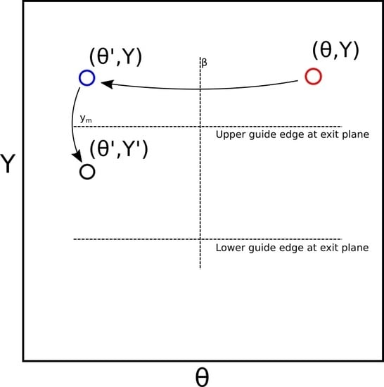
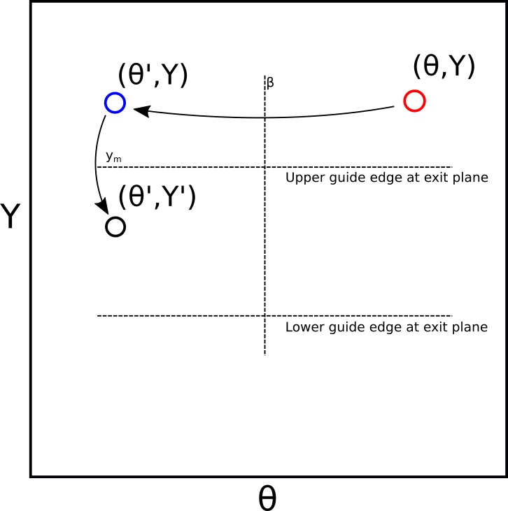
This is perhaps the most useful distinction between acceptance diagram work and conventional ray tracing, and a contributing factor to the speed of the technique. One does not care where the reflection happened—it could be anywhere at all along the length of the mirror—only if it happened. The mirror does not have to be parallel to the beam axis, one assumes the general case that is inclined at a grazing angle relative to the reference axis of the beam (with being the parallel case). If the reflection occurred, then the point in phase space is transformed according to these three steps:
where is the new divergence coordinate of the trajectory relative to the straight beam axis, is the new spatial coordinate, and is the new statistical weight of the trajectory. The and calculations are visualised in Figure 1.
Equation (6) contains the function , which is the supermirror reflectivity at a wavelength and a grazing angle , empirically given by:
where the wavelength- and m-dependent critical angle is given relative to that of total external reflection from atomically smooth nickel with natural isotopic abundances () by:
when the units for are Ångstroms, and for are degrees.
A neutron guide of arbitrary shape is constructed by breaking the system into sections. The beam is first propagated to the exit of the section according to Equation (3), and then for both opposite faces of the guide mirror one performs the application of Equations (4)–(6) in a while() loop until no more point transformations occur. This is done twice in total, once for each acceptance diagram, that is, once in the horizontal plane and once in the vertical plane, in order to model the beam in its entirety.
These equations are fast and simple to deploy. They are prime candidates for fused multiply-add functions (FMA), which are implemented in the GPU hardware and are enabled by default as a compiler optimisation option. An astute reader will note that a while() loop involves branching. According to the basic Cuda introduction, this could slow down the warp dramatically. In practice, however, it is found that particles requiring reflection operations are not isolated cases, and running the reflection steps across the whole warp does not have a measurable impact on the speed, compared to isolating the individual particles requiring reflections. The same result was found for polygons in the original acceptance diagram code [6].
An aperture component can be modelled by setting the statistical weight of the trajectory to zero for trajectories where the position of the neutron y lies beyond the edge of the aperture. This is done by multiplication with a Heaviside function.
A change in axis origin, such as might happen when a guide splits into multiple channels, is modelled by a translation in the y axis by the required amount:
where s is the transverse distance between the centre of the two guide pieces at the join.
Similarly, a rotation of the beam axis—as happens for each section of a curved guide—is modelled by a translation in the axis according to
where is the angle of rotation. Curved guides can then be modelled by repeatedly simulating a straight guide section of the appropriate length (typically 0.5–1 m) using Equations (3)–(6), followed by a rotation with Equation (10), for as many sections as are needed for the curve.
Converging and diverging guides, following elliptic or parabolic shapes, are modelled in a similar way, except that the guides have different entrance and exit widths/heights given by the conic section equations, and no rotation stage.
The final important geometry type is a multi-channel bender. To avoid the use of conditionals, and to allow transporting the neutrons through an accurate simulation of several individual channels, the first step is to divide the phase space into channels and identify which channel the neutron trajectory intersects. Then, for each trajectory, one stores the channel number at the entrance plane. One then shifts the trajectory spatially, so that all trajectories are simulated entering the same bender channel. Optionally, an aperture frame can be modelled that is narrower than the channel width by the channel wafer thickness, to simulate the phase space losses on the front face of the wafers. The neutrons are then transported down a single, narrow channel using the curved guide function described above. Then, at the exit plane, the lateral trajectory shift is applied in reverse so that the trajectories emerge from the correct physical location as though there were multiple channels.
2.2.3. Monitoring and Merging Phase Space
Simulating the trajectories according to the previous two sections will create two matrices in computer memory of 3 columns each, with one matrix representing the horizontal transport efficiency and the other representing the vertical transport efficiency. Beam monitors create a snapshot of the phase space, which are finalised with the statistical weights w at the end of the simulation.
To arrive at a computation of the neutron flux at the sample position, one must merge these two phase spaces and normalise the data to the solid angle illumination of the sample geometry and source brightness of the moderator.
Just as for acceptance diagrams, the moderator brightness is given by:
and we separate the integral of the brightness into two parts, one for each plane, in the small angle approximation, so that
where and are the width and height of the sample, and and are the width and height of the guide exit, separated from the sample by a distance D.
The flux is given by
with the guide system reverse transmission being exactly as discussed in Section 2.1. Now we can see why the reverse tracing method works:
The phase spaces are merged by calculating a total weight , where and are the independently calculated weights of the horizontal and vertical planes respectively. is then simply the sum of divided by the array size. The current is computed from the flux by trivially integrating over the wavelength.
It might be possible, in some future research, to “bootstrap” the computation by exploiting the independence of the horizontal and vertical planes still further. This could be achieved by repeatedly offsetting the and array indices before multiplication, thus artificially expanding the number of 3D samples. However, since the code is already very fast there was no material benefit to exploring this curious idea, and one could easily stumble into a statistical minefield without exercising caution.
3. Benchmarking
3.1. Original NADS Model Tests
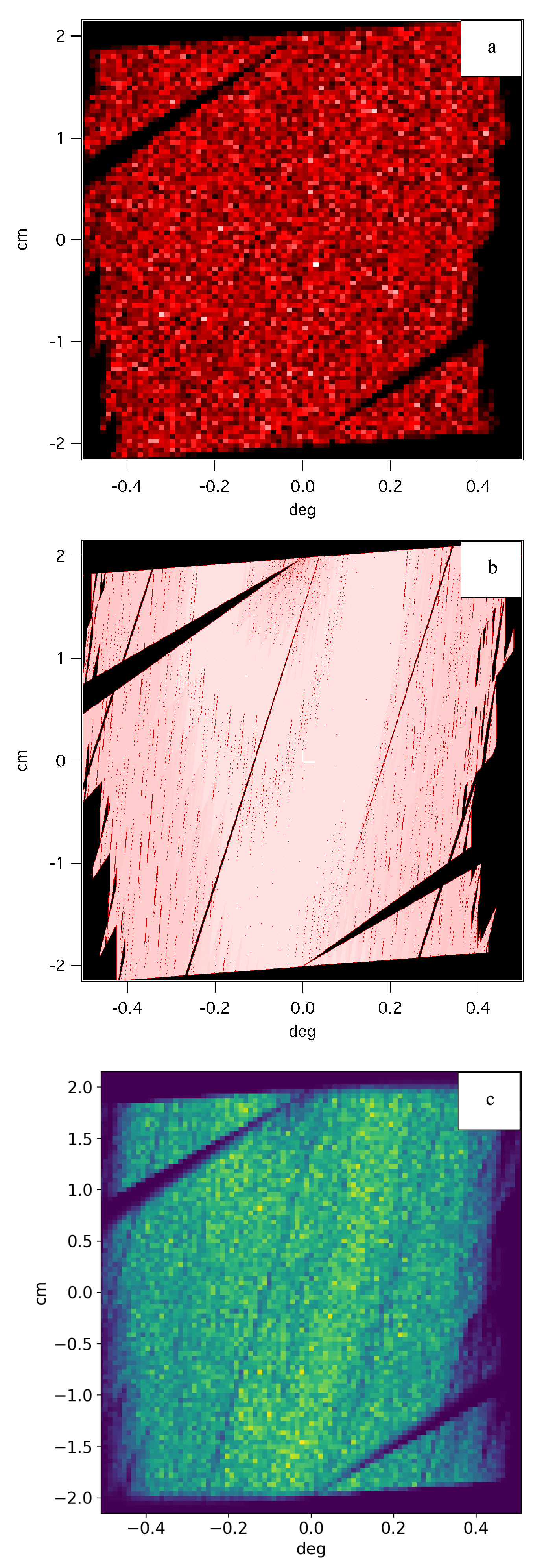
The initial NADS code was extensively tested against several real-world instruments whilst being deployed for the design of ILL H5 guide system [12]. The same benchmarks were repeated for Sandman also. In this current paper, only the D22 instrument will be reported, to show agreement between the three methods—VITESS [3] and NADS after the original paper on that technique [6], and Sandman. The horizontal phase space is reproduced at the position of the first beam attenuator, and shown in Figure 2, where one can see that the agreement between the three methods is good. Minor discrepancies may arise between these packages, typically, in the definition of the m-dependent reflectivity of supermirrors, and corrections for circular apertures vs. square apertures, but these are not significant.
Using a laptop variant of a GTX 1060 GPU in an Alienware R13–R3 laptop from 2017, Sandman can evaluate neutron trajectories per second at the sample position of the D22 SANS instrument, with the maximum collimation distance of 17.6 m. This is the same order of magnitude as the neutron flux on the instrument itself, meaning that the technique demonstrates simulations in real time at the world’s leading neutron source. Whilst this laptop was considered an extreme “gaming” machine at the time, and purchased with the Sandman software application in mind, equivalent performance has become widely available in the subsequent years.
3.2. ESS Design Use Case
In a recent paper [13], a cost optimisation of a spallation source facility was given, in which a re-design was performed on a mature instrument design (“the baseline design”). In that costing paper, the goal was to demonstrate the efficacy of the design methodology, and no real discussion was presented on the use of the software itself. In the present paper, the results illustrate the advantages of the Sandman code. One may modify the geometry, compile and run the code, and obtain the results immediately without having to wait for computing resources to become available and run the job. It allows a scientist to design a system in real time.
Using information in the published reports on the instrument in question, it was possible to reconstruct an accurate model of the phase space in good agreement with those the team generated using McStas. Thereafter, the geometry was interactively modified according to the cost optimisation process [13]. The main thrust of the process is to remove the over-engineering in the supermirror m-values and guide dimensions, and curve the guide to block direct line-of-sight view of the source to save money on shielding. The guidelines are essentially the same as were made available in the form of a design handbook [14] six years prior.
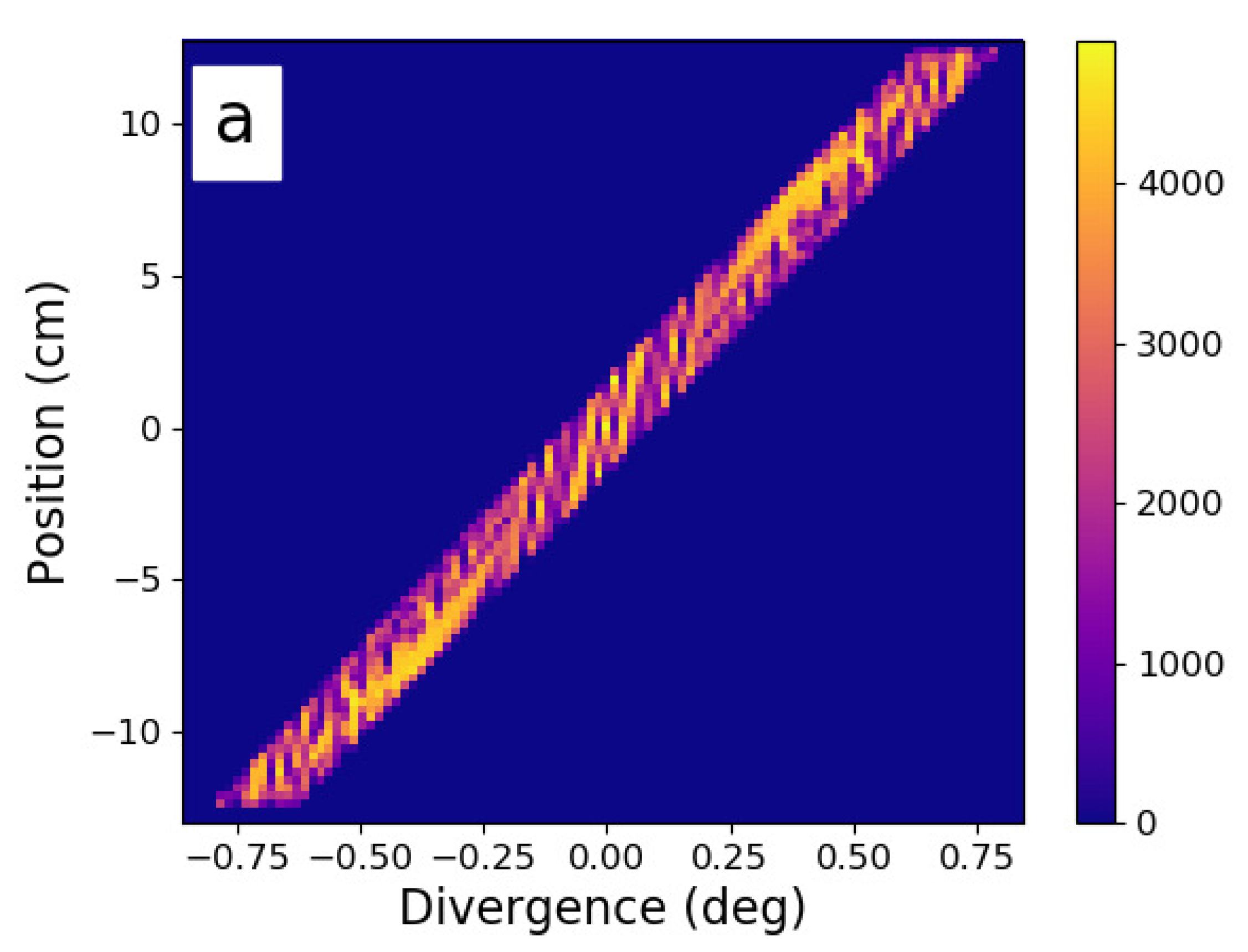
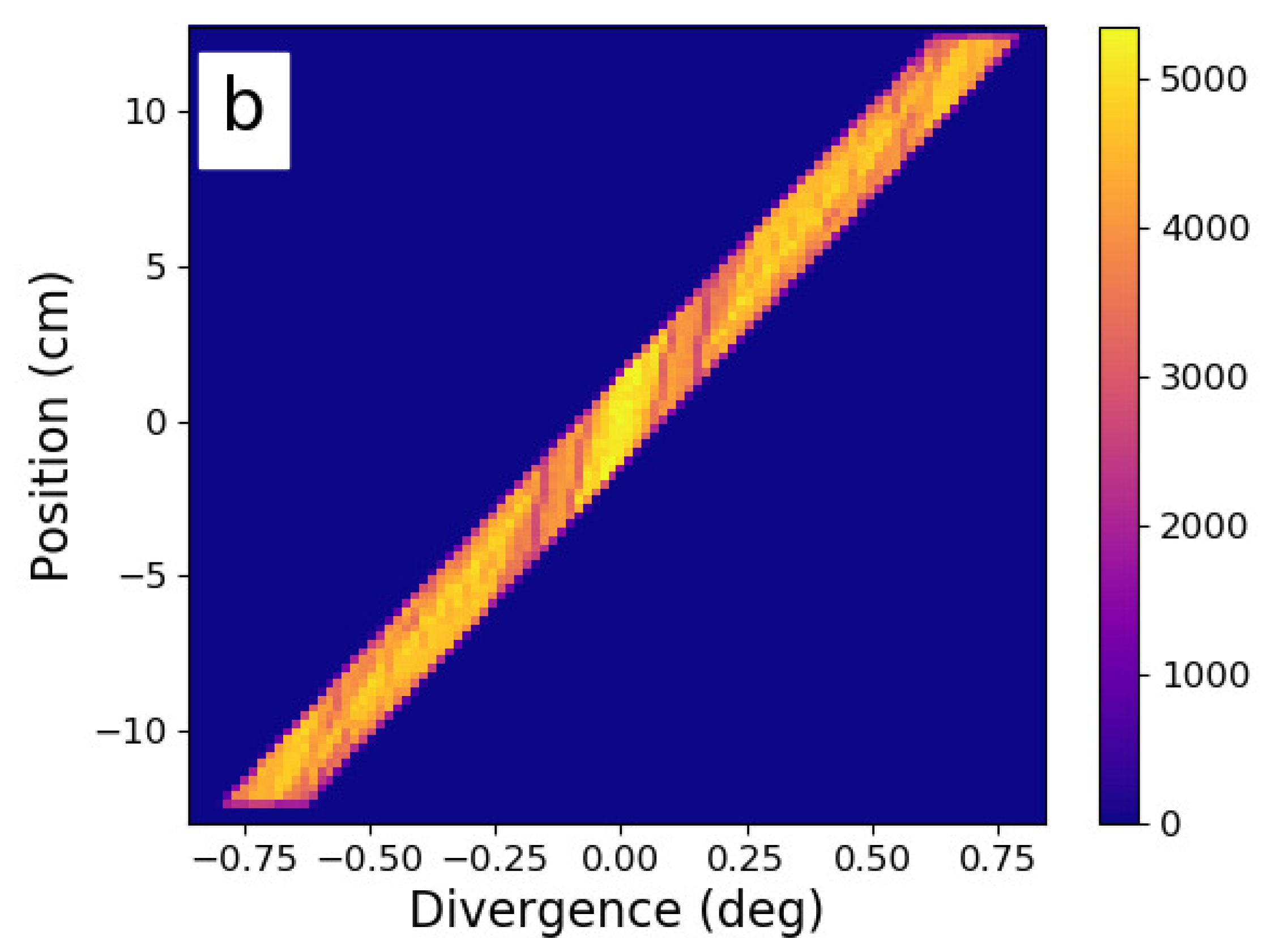
The baseline design had benefited from the input of four scientists and five project managers, over a period of 7 years, and as such, it should certainly be considered mature. Nonetheless, using Sandman for only three days, it was possible to double the instrument performance and reduce the cost of the optics and shielding systems by 40%, from €4.4 M to €2.6 M. Three different variants of the beam were examined, with and without benders to curve out of line of sight, along with two different types of expansion/compression geometry. The best option was then manually refined according to the principles described in the previous work [13]. If one examines the resulting phase space in Figure 3, it is interesting that the brightest parts of the phase space increased only by a small amount. The 200% simulated performance relative to the baseline comes from narrowing the guide geometry and reducing the m-value of the guides to fill in the dark parts of phase space. Both of these measures are certainly not de rigueur in the world of modern neutron guide design and may sound counter-intuitive. On the other hand, elimination of phase space dead areas is fairly straightforward with a good understanding of conic sections—particularly the deliberate manipulation of off-axis effects such as coma [15]. Such phenomena dominate the optical characteristics of systems with spatially extended sources and samples, especially when designers use elliptic shapes to approximate the functionality of parabolæ.
4. Conclusions
A system for simulating neutron guides via adjoint Monte-Carlo sampling of phase space has been described, running on the GPU. It is believed that this represents the fastest possible method for simulating poly-chromatic neutron beams. The count rates using a 2017 laptop approach the same order of magnitude as real world count rates at world-leading instruments, that is, ∼ n/s for D22 at the Institut Laue-Langevin in the highest resolution setting. The code has been benchmarked against existing guide studies from the ILL, and design work from an ESS instrument. For the latter, a use case was presented that shows the main strength of the technique—the interactive design of a guide in real-time, allowing rapid design development as part of a holistic approach to the optical and shielding systems. In so doing, a solution was found with roughly double the performance of an apparently mature design, with cost reductions of almost €2 M, after only three days of work.
Funding
This research received no external funding.
Acknowledgments
The author is very grateful to C. Dewhurst, J. Šaroun, D. Mildner, J. Copley, and J. Cook for interesting and useful discussions.
Conflicts of Interest
The author declares no conflict of interest.
Abbreviations
The following abbreviations are used in this manuscript:
| CPU | Central Processing Unit |
| ESS | European Spallation Source |
| FMA | Fused multiply-add |
| GPU | Graphical Processing Unit |
| NADS | Neutron Acceptance Diagram Shading |
| ILL | Institut Laue Langevin |
| SMs | Streaming Multiprocessors |
References
- Willendrup, P.; Farhi, E.; Lefmann, K. McStas 1.7 a new version of the flexible Monte Carlo neutron scattering package. Physica B 2004, 350, 735. [Google Scholar] [CrossRef]
- Saroun, J.; Kulda, J. Neutron ray-tracing simulations and data analysis with RESTRAX. Proc. SPIE 2004, 5536, 124. [Google Scholar]
- Wechsler, D.; Zsigmond, G.; Streffer, F.; Mezei, F. VITESS: Virtual instrumentation tool for pulsed and continuous sources. Neutron News 2000, 11, 25. [Google Scholar] [CrossRef]
- Bentley, P.M. 2018. Available online: https://github.com/localoptimum/sandman (accessed on 16 June 2020).
- Mildner, D. Acceptance Diagrams for Curved Neutron Guides. Nucl. Instrum. Methods Phys. Res. Sect. A 1990, A290, 189. [Google Scholar] [CrossRef]
- Bentley, P.M.; Andersen, K.H. Accurate simulation of neutrons in less than one minute Pt. 1: Acceptance Diagram Shading. Nucl. Instrum. Methods Phys. Res. Sect. A 2008, 602, 564. [Google Scholar] [CrossRef]
- Coveyou, R.R.; Cain, V.R.; Yost, K.J. Adjoint and Importance in Monte Carlo Application. Nucl. Sci. Eng. 1967, 27, 219–234. [Google Scholar] [CrossRef]
- Desorgher, L.; Lei, F.; Santin, G. Implementation of the reverse/adjoint Monte Carlo method into Geant4. Nucl. Instrum. Methods Phys. Res. Sect. A 2010, 621, 247–257. [Google Scholar] [CrossRef]
- 2020. Available online: https://developer.nvidia.com/ (accessed on 16 June 2020).
- Precision and Performance: Floating Point and IEEE 754 Compliance for NVIDIA GPUs; Technical Report; TB-06711-001_v11.0; NVIDIA: Santa Clara, CA, USA, 2020.
- Weisstein, E.W. Triangle Point Picking from MathWorld—A Wolfram Web Resource. 2020. Available online: http://mathworld.wolfram.com/TrianglePointPicking.html (accessed on 16 June 2020).
- Bentley, P.M.; Boehm, M.; Sutton, I.; Dewhurst, C.D.; Andersen, K.H. Global optimisation of an entire neutron guide hall. J. Appl. Cryst. 2011, 44, 483. [Google Scholar] [CrossRef]
- Bentley, P.M. Instrument Suite Cost Optimisation in a Science Megaproject. J. Phys. Commun. 2020, 4, 045014. [Google Scholar] [CrossRef]
- Zendler, C.; Santoro, V.; Ansell, S.; Cherkashyna, N.; Rodriguez, D.M.; Cooper-Jensen, C.; DiJulio, D.; Bentley, P.M. European Spallation Source Neutron Optics and Shielding Guidelines, Requirements and Standards; Technical Report ESS-0039408; European Spallation Source: Lund, Sweden, 2015. [Google Scholar]
- Bentley, P.M.; Kennedy, S.J.; Andersen, K.H.; Rodriguez, D.M.; Mildner, D.F.R. Correction of optical aberrations in elliptic neutron guides. Nucl. Instrum. Methods Phys. Res. Sect. A 2012, 693, 268–275. [Google Scholar] [CrossRef] [Green Version]
Figure 1.
Illustration of the reflection of a phase space point in an inclined mirror plane, according to Equations (4) and (5).
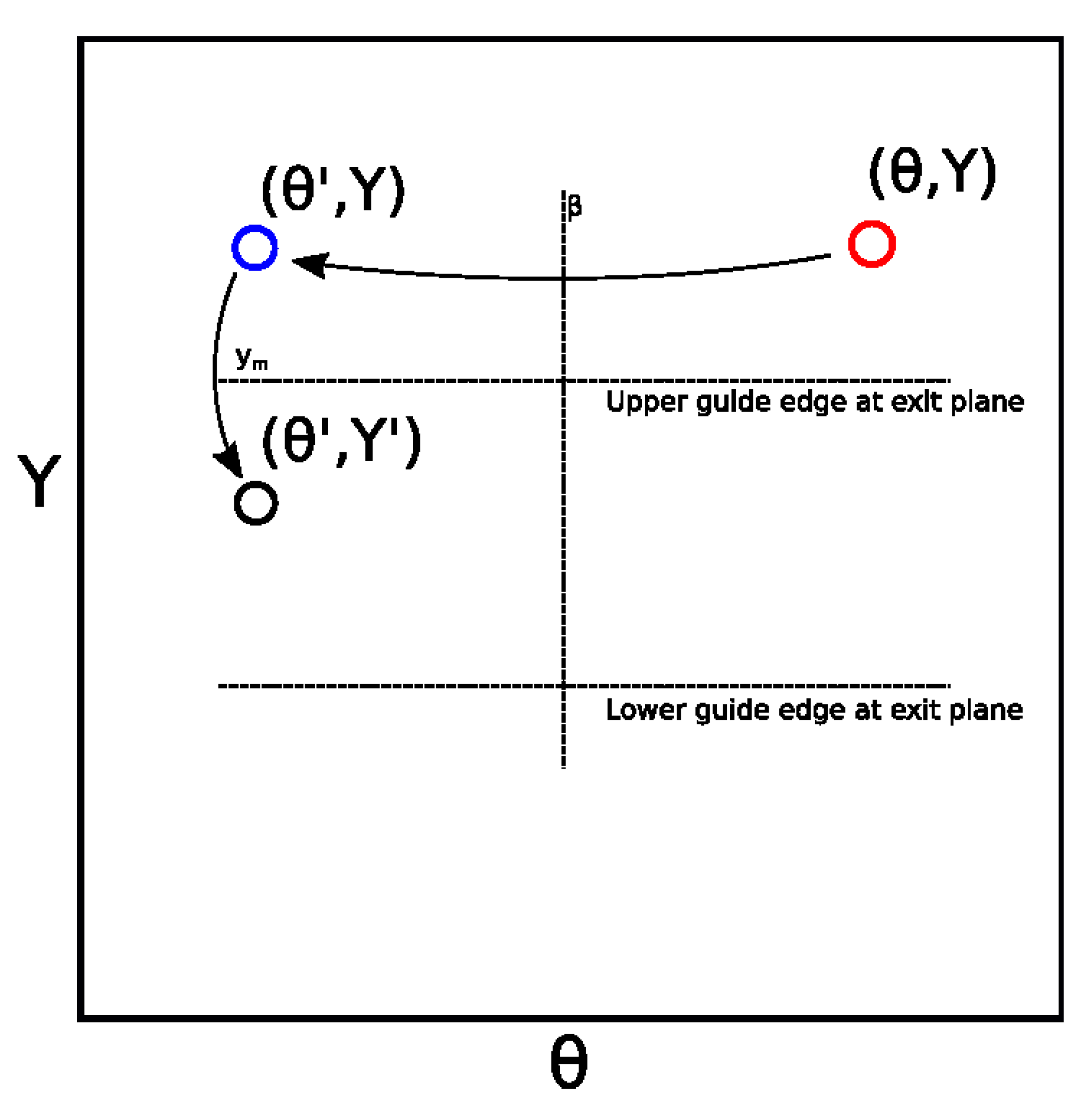
Figure 2.
Simulation of the D22 instrument phase space at the attenuator position, computed with: (a) VITESS, from Reference [6]; (b) Acceptance Diagram Shading, from Reference [6]; (c) Sandman, the present work.

Figure 3.
Redesign of a mature ESS instrument concept, and the improvements in phase space that were obtained. Here we see the horizontal phase space at the sample position. (a) the instrument baseline, with ∼7 years of development work. (b) the results of three days of redesign work using Sandman, providing double the performance and a €1.8 M cost reduction [13].


© 2020 by the author. Licensee MDPI, Basel, Switzerland. This article is an open access article distributed under the terms and conditions of the Creative Commons Attribution (CC BY) license (http://creativecommons.org/licenses/by/4.0/).
Share and Cite
MDPI and ACS Style
Bentley, P. Accurate Simulation of Neutrons in Less Than One Minute Pt. 2: Sandman—GPU-Accelerated Adjoint Monte-Carlo Sampled Acceptance Diagrams. Quantum Beam Sci. 2020, 4, 24. https://0-doi-org.brum.beds.ac.uk/10.3390/qubs4020024
AMA Style
Bentley P. Accurate Simulation of Neutrons in Less Than One Minute Pt. 2: Sandman—GPU-Accelerated Adjoint Monte-Carlo Sampled Acceptance Diagrams. Quantum Beam Science. 2020; 4(2):24. https://0-doi-org.brum.beds.ac.uk/10.3390/qubs4020024
Chicago/Turabian StyleBentley, Phillip. 2020. "Accurate Simulation of Neutrons in Less Than One Minute Pt. 2: Sandman—GPU-Accelerated Adjoint Monte-Carlo Sampled Acceptance Diagrams" Quantum Beam Science 4, no. 2: 24. https://0-doi-org.brum.beds.ac.uk/10.3390/qubs4020024