The Large-Area Detector for Small-Angle Neutron Scattering on iMATERIA at J-PARC
by
 ,
,
Yohei Noda
1, 
Hideki Izunome
2,
Tomoki Maeda
1,
Takumi Inada
1,
Satoru Ueda
1 and
Satoshi Koizumi
1,* 1
Institute of Quantum Beam Science, Ibaraki University, 162-1 Shirakata, Tokaimura, Nakagun, Ibaraki 319-1106, Japan
2
Hitachi Denki Kogyo Co., Ltd. 1270-17 Tomecho, Hitachi, Ibaraki 319-1231, Japan
*
Author to whom correspondence should be addressed.
Quantum Beam Sci. 2020, 4(4), 32; https://0-doi-org.brum.beds.ac.uk/10.3390/qubs4040032
Submission received: 31 July 2020
/
Revised: 7 September 2020
/
Accepted: 15 September 2020
/
Published: 23 September 2020
(This article belongs to the Special Issue New Trends in Neutron Instrumentation)
Abstract
:An area detector with a central hole structure was built up for small-angle neutron scattering (SANS) on the iMATERIA instrument at Japan Proton Accelerator Research Complex (J-PARC). Linear position-sensitive detector tubes filled with 3He gas were arranged in three layers leaving a central hole. As a result of the calibration process, a SANS measurement with wide q-range from 0.007 Å−1 to 4.3 Å−1 was achieved in double-frame operation, supplying neutrons with wavelengths from 1 Å to 10 Å. As a merit of this central hole structure, neutron transmission can be measured simultaneously to reduce experimental time and effort. This is ideal for time-resolved studies, in which the sample transmission can be time-dependent, throughout the whole experiment. Additionally, the data storage system in ‘event mode’ format provides an excellent platform for such time-resolved experiments.
1. Introduction
Small-angle neutron scattering (SANS) has long been effectively used for studying mesoscopic and microscopic structures of polymeric, biological, and metallurgic materials. A variety of SANS spectrometers are in operation at neutron facilities. For example, as a reactor type-instrument, there are GP-SANS and BIO-SANS at Hi Flux Isotope Reactor (HFIR) [1], 45m-SANS(NG-3), 30m-SANS (NG-7), 30m-SANS (NG-B), and 10m-SANS at National Institute of Standards and Technology(NIST) [2], D11 [3], D22, and D33 [4] at Institut Laue-Langevin (ILL), KWS-1 [5], KWS-2 [6], and SANS-1 [7] at Forschungsreaktor München II (FRM-II), QUOKKA [8,9] and BILBY [10] at Australian Nuclear Science and Technology Organisation (ANSTO), 40m-SANS at High-Flux Advanced Neutron Application Reactor (HANARO) [11], SANS-J-II [12,13] and SANS-U [14] at Japan Research Reactor No. 3 (JRR-3). As a spallation source instrument, there are EQ-SANS [15,16] at Sapallation Neutron Source (SNS), Sans-2d [17] at ISIS, TAIKAN [18,19] at J-PARC, and SKADI and LoKI at European Spallation Source (ESS) (under construction) [20]. SANS instruments at pulsed spallation sources that typically employ the time-of-flight (TOF) approach to utilize neutrons over a wide wavelength range simultaneously. Hence, wide dynamic q-range can be obtained by a single measurement, as indicated by the pioneering works [21,22,23].
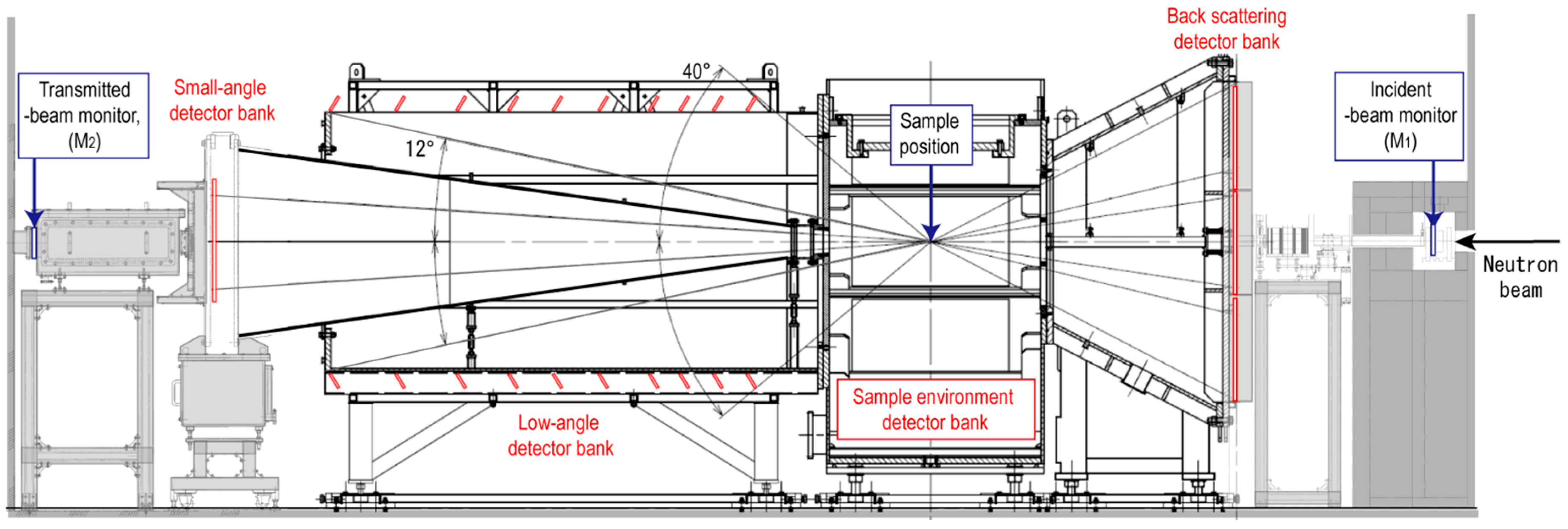
iMATERIA [24,25] at J-PARC’s Materials and Life Science Facility [25,26,27] is a versatile neutron scattering spectrometer with a large number of position-sensitive detectors (PSDs), classified into four detector banks; back scattering (BS, 2θ ≈ 180°), sample environment (SE, 2θ ≈ 90°), large angle (LA, 12° < 2θ < 40°), and small angle (SA, 0.6° < 2θ < 5.5°) detector banks (Figure 1). Here, 2θ is the scattering angle. We have engaged in upgrading iMATERIA to make it more suitable for SANS. The original area SANS detector at iMATERIA was a simple array of PSD tubes, with the center covered with a cadmium beam stop. However, high-intensity fast neutrons from the J-PARC neutron source transmitted through this beam stop to paralyze the central PSD tubes. In order to avoid this situation, we newly designed an area detector with a central hole, a similar fashion to TAIKAN at J-PARC [18,19]. In this article, we report the design, calibration process, and performance of the newly upgraded SANS area detector.
2. Instrumentation
2.1. 3He PSD Tube
We employed 3He PSD tubes (outer diameter: ϕ12.7 mm, 3He gas pressure: 20 atm) by Toshiba Electron Tube and Devices Co., Ltd. (Tochigi, Japan). The tube wall is made of 0.25 mm thick stainless steel.
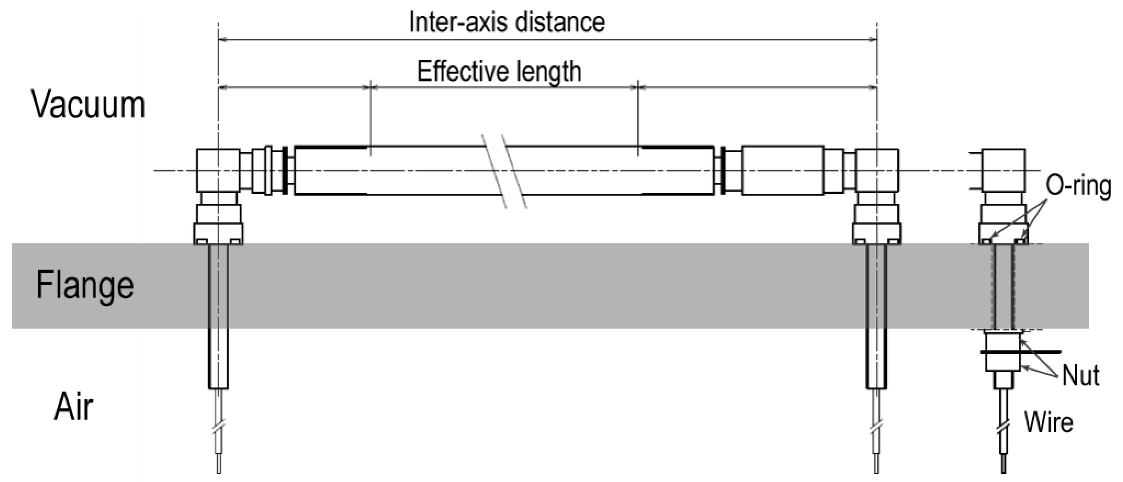
In many neutron scattering instruments, including almost all SANS instruments, the space between the sample and detectors is evacuated in order to minimize scattering of neutrons by air. At the same time, we need to apply high voltages (~1680 V) to the PSD tubes. To avoid high-voltage discharge, the conductive wires should be placed in atmospheric conditions. As shown in Figure 2, both ends of type E6867 PSD tube are designed to fit the flange of vacuum chamber by use of O-ring. Consequently, the active length of the PSD tube can be located in vacuum conditions, while the conductive wires are located in atmospheric conditions. This PSD tube (type E6867) circumvents the high-voltage discharge problem ingeniously, and is free from background from the atmospheric chamber, which is difficult to avoid to with some other types of PSD tubes. The lengths of the 3He PSD tubes are listed in Table 1.
2.2. 3He PSD Tube Arrangement
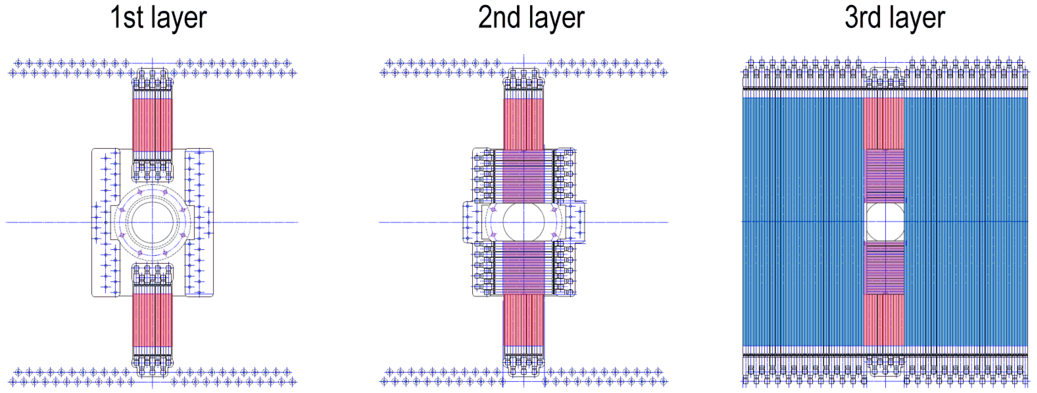
The area detector, with a central hole, is realized by PSD tubes with three different lengths arranged in three layers (Figure 3). The first layer of PSD tubes (E6867-127) is arranged vertically in the top and bottom blocks, above and below the straight-through beam. Then, as a second layer, PSD tubes (E6867-100) are arranged horizontally, covering the ineffective region of the first layer. Finally, PSD tubes (E6867-600) were arranged vertically, covering over the ineffective region of the PSD tubes in the second layer. The first and second layers are placed 14.5 mm and 29 mm downstream of the third layer, respectively. The 40 mm-thick detector flange have thin area for accommodating the first and second layer PSDs. Prior to manufacturing the flange, the stresses and deflections caused by the chamber evacuation were simulated by a finite-element-analysis software, ANSYS. By this simulation, it was confirmed that introduction of rib on the atmospheric side of the flange can reduce the stresses and deflections to allowable level. Figure 4 indicates the photograph of the built-up area detector.
2.3. Readout Module and Data Processing Software
To determine the position of the neutron capture, we employed a neutron encode (NEUNET) module (Techno AP Co. Ltd., Ibaraki, Japan) [26,28], commonly employed in J-PARC’s Material and Life Science Facility. The NEUNET module is based on the charge-division method for neutron position detection and is designed for TOF experiments at spallation neutron sources. The neutron capture event generates pulse currents in both terminals of the PSD tubes. The pulse current signal is amplified by a charge amplifier (AMP 97 board), and then the NEUNET module outputs the ID number of PSD tube (8 bit), the observed pulse heights at both terminals (12 bit × 2) and the time of the event. The full detail of the data format is described in the literature [28]. For synchronizing the neutron detection with neutron pulse, a 25 Hz trigger signal from the proton accelerator is supplied to the NEUNET module. The output data from the NEUNET module are registered on a large-scale storage system by use of DAQ-Middleware [26,29]. For data reduction from the event-mode data, ‘iM analysis’ software has been developed. Users can perform background subtraction, counting efficiency correction and circular/sector averaging to obtain a one-dimensional scattering profile on a LINUX-based workstation.
3. Data Processing
3.1. Position Sensitive Detection by Charge Division Method
We employed the charge division method for the position-sensitive detection of incoming neutrons into PSD tubes. When a neutron enters into a PSD tube, it is captured by a 3He nucleus inside the tube to generate a charge cloud by the following reaction:
3He + neutron → 3H + proton + 764 keV.
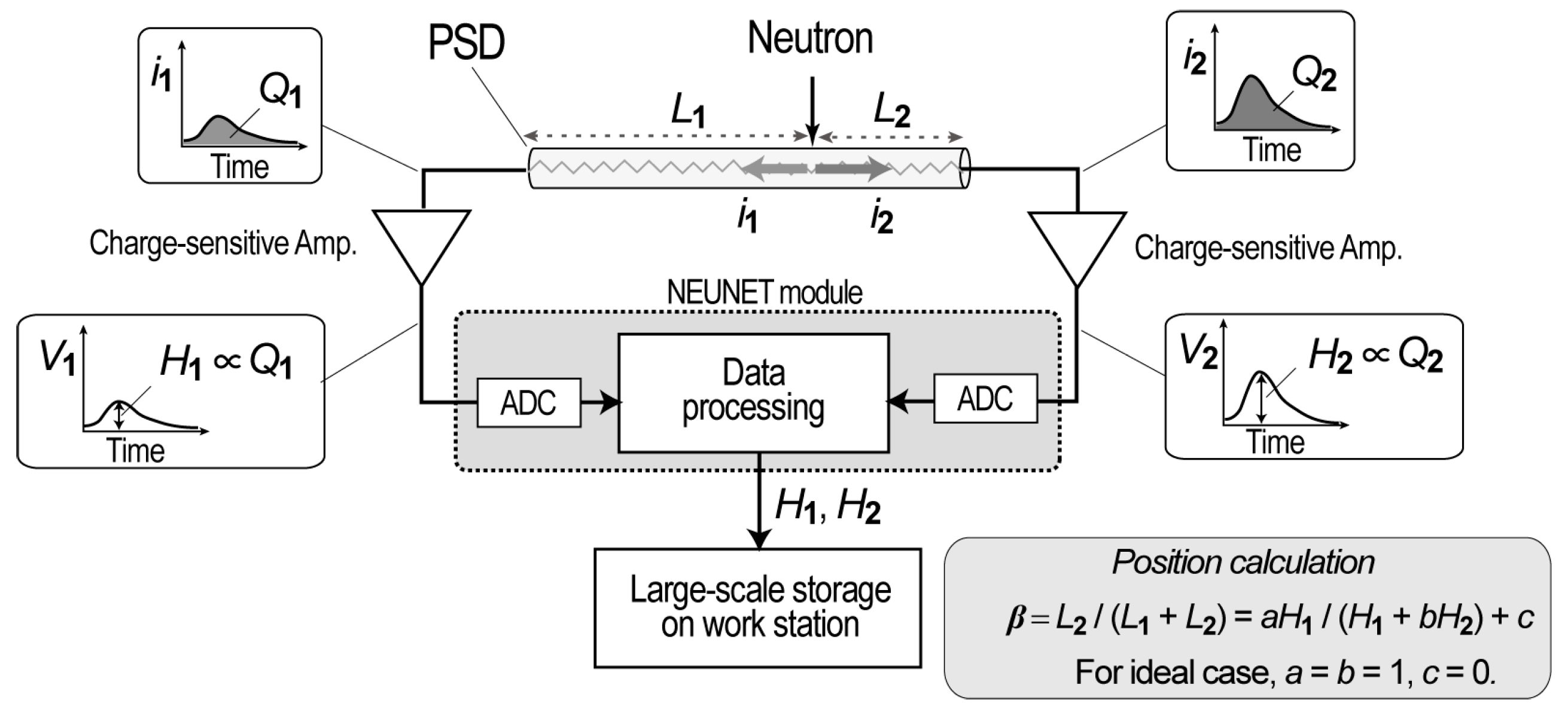
As a result of the high voltage, the charge cloud generates an electric current, which is divided into two distinct pathways, as indicated by i1 and i2 in Figure 5. The ratio of i1 and i2 is determined by the inverses of the pathway resistances through which they flow. If the cross-sectional area of the cathode wire is constant, the resistance is hence proportional to the length of the each of the pathways. Therefore, i1/i2 equals to L2/L1. Here L1 and L2 are the length of the pathways in which i1 and i2 flow, respectively. For evaluating i1/i2, the small pulse current resulting from neutron irradiation is enhanced by a charge-sensitive amplifier. The time evolution of the signal is then converted to digital data. Finally, the pulse heights of the temporal profiles (H1 and H2) are obtained for both pathways. By use of β (= L2/(L1 + L2)), the position of detected neutron (r) is calculated as follows:
r = βr1 + (1 − β)r2.
Here, r1 and r2 are the positions of both ends of the PSD tube. β is related to H1 and H2 as follows:
β = aH1/(H1 + bH2) + c.
Here, a, b, and c are correction parameters, which should be determined by calibration for each PSD tube. It will be discussed later. In ideal case (a = b = 1 and c = 0), β = H1/(H1 + H2) is satisfied.
3.2. Event-Mode Data Histograming
Event-mode data for each detection events are composed of PSD number, pulse heights (H1 and H2), and a detection time. A merit of event-mode data is that we can repeatedly select a period for analysis, since the event-mode data contains absolute time of detection for every single event. However, in return for this advantage, event-mode data collection consumes much more memory. For example, typical SANS measurement (30 min under 500 kW operation) requires about 1 GB.
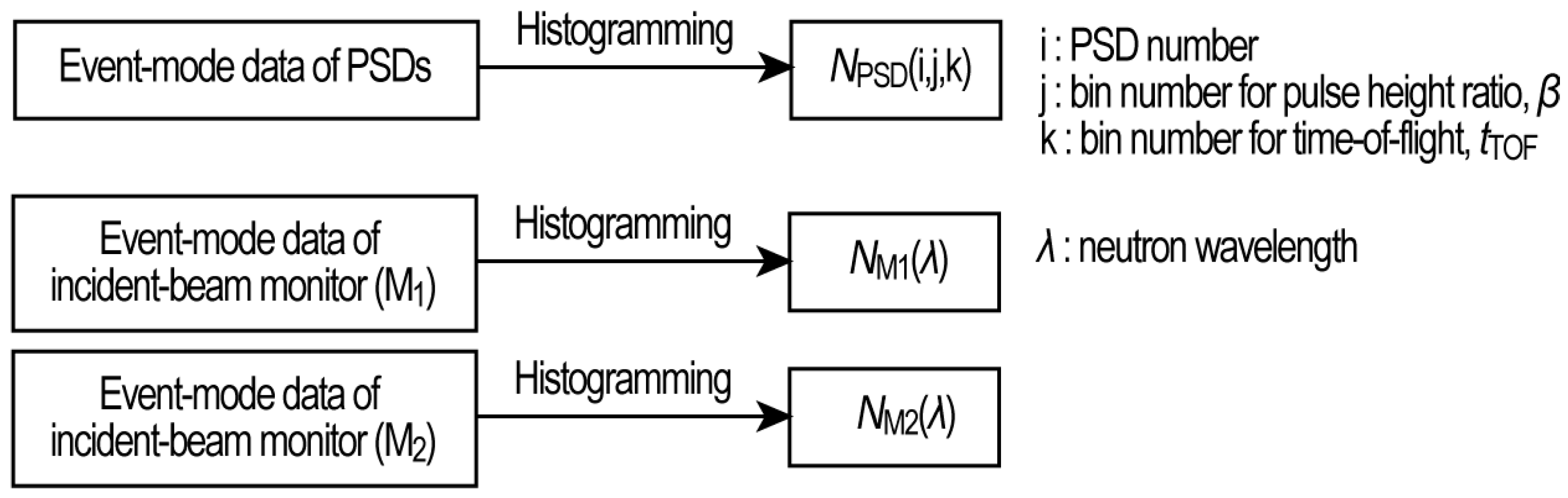
As a first data-processing step, a three-dimensional histogram array, NPSD(i,j,k) is constructed from the event data (Figure 6, 1st line). The indices i, j, and k label PSD number, pulse height ratio (β), and time-of-flight (tTOF), respectively. The neutron counts observed at the incident-beam monitor (M1) and transmitted-beam monitor (M2) are also stored as event-mode data. From these event-mode data, one-dimensional histogram arrays NM1(λ) and NM2(λ) are obtained (Figure 6, 2nd and 3rd lines). Here, the neutron wavelength λ is given by λ = (h/mn) (tTOF/L), where h is Planck’s constant, mn is neutron mass, and L is neutron flight path length. (L = 23.14 m for M1, and 32.37 m for M2).
3.3. Calculation of Geometric Arrays
The following geometric arrays are dependent only on the geometric conditions of the area detector. For indices i and j, the xyz coordinates of the neutron detection position are calculated using the following equation:
x(i, j) = β(j)x1(i) + (1 − β(j))x2(i),
y(i, j) = β(j)y1(i) + (1 − β(j))y2(i),
z(i, j) = β(j)z1(i) + (1 − β(j))z2(i).
y(i, j) = β(j)y1(i) + (1 − β(j))y2(i),
z(i, j) = β(j)z1(i) + (1 − β(j))z2(i).
Here, r1(i) (= (x1(i), y1(i), z1(i))) and r2(i) (= (x2(i), y2(i), z2(i))) are the positions of both ends of the PSD tube labeled ‘i’. The origin of the xyz coordinate is set at the sample position. The z-axis is set along the incident beam line. Then, the scattering angle, 2θ(i, j) is given by the following equation:
The solid angle for each channels, ∆Ω(i,j) is calculated as follows:
Here, 2R is effective diameter of the PSD tubes (=12.2 mm), and px and py is pixel width along the PSD tubes [30]. The neutron wavelength, λ(i, j, k) is given by the following equation:
Here, L1 is the flight path length from the moderator to the sample (26.50 m). The scattering vector magnitude, q is defined as q = (4π/λ)sinθ. For each channel, a three-dimensional array of q, Q(i,j,k) can be calculated as follows:
3.4. One-dimensional Profile Calculation
The one-dimensional profile I(q) is given by the following equation:
where Is(q) and Ib(q) indicate the SANS profiles for sample and background (empty cell) measurements, respectively. Is(q) and Ib(q) are calculated from the event data histograms by the following equations:
I(q) = Is(q) − Ib(q),
Here, K is a prefactor for obtaining absolute intensity in cm−1, and ds is a sample thickness. The subscripts ‘s’ and ‘b’ on the event data histogram arrays indicate sample and background (empty cell) measurement, respectively. The subscript ‘c’ means closed-beam measurement by locating a B4C block at the sample position. W(i, j, k, n) is an indicator function for the 1D profile calculation
The q sequence defined as follows:
q(n) = q0 αn.
Here, n is bin number of q, q0 is initial value of q, and α is common ratio (we employ α = 1.025). M(i,j,k) is an indicator function for mask. M(i,j,k) = 1 for channels which should be considered, and M(i,j,k) = 0 for channels which should be neglected. M(i,j,k) is the product of the following three sub-functions:
Here, Mg(i,j) is a geometric mask, used for neglecting ineffective regions of the PSD tubes. Mλ(λ) is a neutron wavelength mask. Mt(k) is a mask for time. A sensitivity correction function, η(i,j,k), is the product of the following two sub-functions:
ηPSD(i) is the sensitivity of each PSD tube. ηλ(λ) is a neutron wavelength-dependent sensitivity, which is assumed to be common for all the PSD tubes. Since they have the same 3He gas pressure and tube diameter, their detection efficiency should be similar. Although slight variations in the wavelength-dependent sensitivity are expected among the PSD tubes, this approach works well as shown later in Section 4.3. Ts(θ, λ) is a transmission considering the effect of scattering-angle dependent thickness [31,32], calculated as follows:
Here, Ts0(λ) is a transmission for θ = 0 as determined by the monitor counts of M1 and M2 as follows:
The above transmission parameters relate to sample measurement. For background measurement, Tb(θ, λ) and Tb0(λ) are calculated in a similar manner. The subscript of event data histogram ‘o’ means a background measurement without an empty cell. If there is no sample cell, Tb0(λ) = 1.
4. Results and Discussion
4.1. Calibration of Position Detection
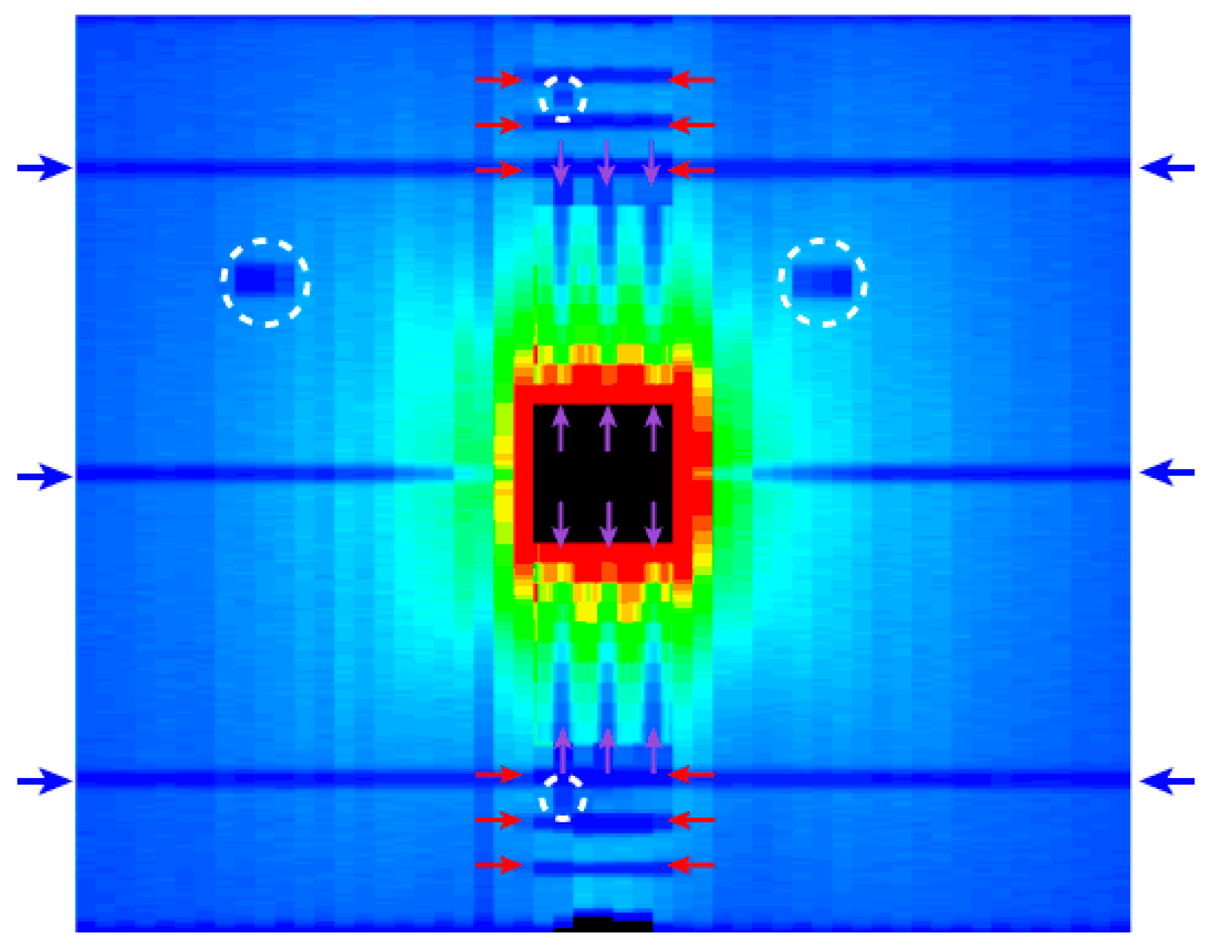
The position of neutron detection is calculated by Equations (3) and (4), based on the charge-division method. For determining the correction factors (ai, bi and ci), we conducted a calibration measurement using a cadmium mask plate as follows: three cadmium strips (0.5 mm thickness and 10 mm width) were fixed on an aluminum plate, across the each of the PSD tubes. The distance between the strips is 200 mm for E6867-600 and 30 mm for E6867-127 and E6867-100. The scattered neutrons from a 1 mm glassy carbon standard were observed with the mask plate just in front of the area detector. Figure 7 shows the two-dimensional distribution of neutron counts on the area detector with accumulating neutron events for all tTOF (the ‘real-space histogram’). The neutron count histogram along the PSD tube shows three dips due to the cadmium mask strips. After the adjustment of the correction factors, ai, bi and ci, the positions of the dips were aligned in straight lines as shown in Figure 7. The image in Figure 7 was obtained with the ai, bi, and ci parameters after this calibration process. The determined ai, bi, and ci parameters were then registered in the configuration file of the data reduction software.
4.2. Efficiency of Each PSD, ηPSD(i)
Figure 8 shows the neutron count as a function of the position along a typical PSD tube. As an incoherent scatterer, 1 mm-thick H2O was placed at the sample position. The neutron count is flat except for narrow regions at both ends. Based on this observation, the sensitivity along the PSD tubes was regarded as homogeneous. The narrow region with low sensitivity at both ends was omitted by use of geometrical mask, Mg(i,j). Where there were slight sensitivity variations for each PSDs, a correction factor ηPSD(i) was introduced. We determined ηPSD(i) by comparing the neutron counts for each PSD tube, for the measurement of incoherent scattering due to H2O, and registered them in the configuration file of the data reduction software.
4.3. Neutron Wavelength Dependence of Detection Efficiency, ηλ(λ)
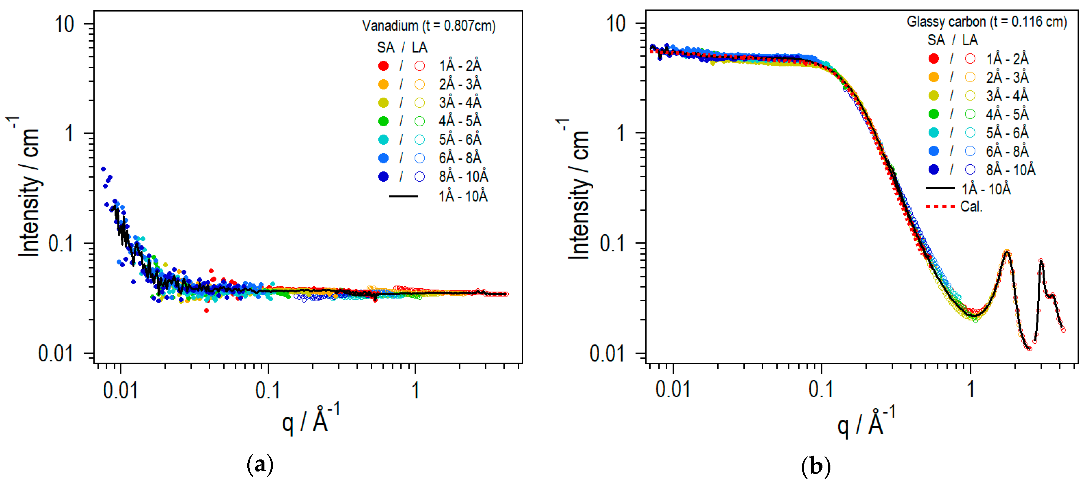
For achieving wide q-range by combining SANS contribution with various λ, we should properly apply λ-dependent terms (TS(λ) and ηλ(λ)) in Equation (10), otherwise the obtained profile is distorted artificially. For this purpose, we measured scattering from vanadium, which shows q-independent flat region due to incoherent scattering at q > 0.03 Å−1.
As a calibration process, with tentatively setting ηλ(λ) = 1, I(q) for limited λ-region was calculated by use of Mλ(λ). Then, we shifted obtained I(q) profiles to obey a common single I(q) profile. As an inverse of this shift factor, we determined ηλ(λ). Figure 9a shows the one-dimensional profile obtained with the determined ηλ(λ). The determined ηλ(λ) is registered in the configuration file of the data reduction software.
Figure 9b shows the one-dimensional profile from a glassy-carbon standard [33] supplied by Dr. Ilavsky (Advanced Photon Source at Argonne National Laboratory). Here, the ηλ(λ) determined by the vanadium measurement were applied. The calculated 1D profiles with different λ-ranges overlapped each other to form a totally combined profile for λ = 1 Å − 10 Å as shown by a thick black line. The coincidence between the different λ-range profiles was pretty good, but not perfect probably due to a weak inelastic effect. The totally combined profile agreed well with the absolute intensity profile measured by Dr. Ilavsky, as shown by a red dotted line. Here, we adjusted the prefactor for absolute intensity (K in Equation (10)). The determined K were registered on the configuration file of the data reduction software. For different collimation conditions, a measurement with the glassy carbon standard for K determination should be repeated. In Figure 9b, the 1D profile from LA detector bank (q = 0.13 Å−1 − 4.3 Å−1) clearly shows diffraction peaks due to the stacking of hexagonal carbon layers. The TOF-SANS approach provides structural information all the way from the mesoscopic scale to the atomic scale in a single experiment.
5. Conclusions
An area detector, with a central hole structure, was built up for circumventing the loss of central PSDs caused by intense irradiation by fast neutrons. As a result of the calibration process, a wide q-range SANS profile from 0.007 Å−1 to 4.3 Å−1 was obtained from a single measurement. In addition, the central hole structure enables a simultaneous transmission measurement, which reduces experimental time and effort and is ideal for time-resolved studies. Additionally, the data storage system with the ‘event-mode data’ format provides an excellent platform for the time-resolved studies. The time-division width for analysis can be chosen, varied, and reset even after the measurement. The hardware and software conditions for TOF-SANS experiments have been completed for users. Since the introduction on January 2016, the area detector has been in stable operation over four years, and utilized in studies of a variety of industrial materials, such as polymer electrolyte membrane [34,35,36]. Table 2 summarizes the specification of the SANS detector. As a future prospect, we are continuously engaged in the effort for extending the q-range to lower and higher q values.
Author Contributions
Conceptualization: S.K.; methodology: Y.N. and S.K.; data curation and formal analysis: Y.N., H.I., T.M., T.I., and S.U.; investigation: Y.N., H.I., T.M., T.I., S.U., and S.K.; resources: Y.N. and S.K.; writing—original draft preparation: Y.N.; writing—review and editing: S.K.; supervision: S.K.; project administration: S.K. All authors have read and agreed to the published version of the manuscript.
Funding
This research was financially supported by Ibaraki Prefecture (Leading Research Project of Ibaraki Neutron Beam line).
Acknowledgments
SANS experiments were carried out at BL20 iMATERIA in J-PARC MLF (proposal no. 2016PM0005, 2017PM0001, 2018PM0005, 2019PM3003, and 2020PM3004). We appreciate support from iMATERIA staff. We appreciate Jan Ilavsky (Advanced Photon Source at Argonne National Laboratory) for supplying a glassy carbon standard with the scattering data for calibration. We appreciate Robert A. Robinson (University of Wollongong and Ibaraki University) for helpful discussions.
Conflicts of Interest
The authors declare no conflict of interest.
References
- Heller, W.T.; Cuneo, M.J.; DeBeer-Schmitt, L.M.; Do, C.; He, L.; Heroux, L.; Littrell, K.; Pingali, S.V.; Qian, S.; Stanley, C.B.; et al. The suite of small-angle neutron scattering instruments at Oak Ridge National Laboratory. J. Appl. Crystallogr. 2018, 51, 242–248. [Google Scholar] [CrossRef]
- NIST Center for Neutron Research, Neutron Instruments. Available online: https://www.nist.gov/ncnr/neutron-instruments (accessed on 22 September 2020).
- Lindner, P.; Schweins, R. The D11 Small-Angle Scattering Instrument: A New Benchmark for SANS. Neutron News 2010, 21, 15–18. [Google Scholar] [CrossRef]
- Dewhurst, C.; Grillo, I.; Honecker, D.; Bonnaud, M.; Jacques, M.; Amrouni, C.; Perillo-Marcone, A.; Manzin, G.; Cubitt, R. The small-angle neutron scattering instrument D33 at the Institut Laue–Langevin. J. Appl. Crystallogr. 2016, 49, 1–14. [Google Scholar] [CrossRef]
- Feoktystov, A.; Frielinghaus, H.; Di, Z.; Jaksch, S.; Pipich, V.; Appavou, M.-S.; Babcock, E.; Hanslik, R.; Engels, R.; Kemmerling, G.; et al. KWS-1 high-resolution small-angle neutron scattering instrument at JCNS: Current state. J. Appl. Crystallogr. 2015, 48, 61–70. [Google Scholar] [CrossRef]
- Houston, J.E.; Brandl, G.; Drochner, M.; Kemmerling, G.; Engels, R.; Papagiannopoulos, A.; Sarter, M.; Stadler, A.; Radulescu, A. The high-intensity option of the SANS diffractometer KWS-2 at JCNS – characterization and performance of the new multi-megahertz detection system. J. Appl. Cryst. 2018, 51, 323–336. [Google Scholar] [CrossRef]
- Mühlbauer, S.; Heinemann, A.; Wilhelm, A.; Karge, L.; Ostermann, A.; Defendi, I.; Schreyer, A.; Petry, W.; Gilles, R. The new small-angle neutron scattering instrument SANS-1 at MLZ—Characterization and first results. Nucl. Instrum. Methods Phys. Res. Sect. A Accel. Spectrometers Detect. Assoc. Equip. 2016, 832, 297–305. [Google Scholar] [CrossRef] [Green Version]
- Wood, K.; Jeffries, C.M.; Knott, R.B.; Sokolova, A.V.; Jacques, D.; Duff, A.P. Exploring the structure of biological macromolecules in solution using Quokka, the small angle neutron scattering instrument, at ANSTO. Nucl. Instrum. Methods Phys. Res. Sect. A Accel. Spectrometers Detect. Assoc. Equip. 2015, 798, 44–51. [Google Scholar] [CrossRef]
- Wood, K.; Mata, J.; Garvey, C.J.; Wu, C.-M.; Hamilton, W.A.; Abbeywick, P.; Bartlett, D.; Bartsch, F.; Baxter, P.; Booth, N.; et al. QUOKKA, the pinhole small-angle neutron scattering instrument at the OPAL Research Reactor, Australia: Design, performance, operation and scientific highlights. J. Appl. Crystallogr. 2018, 51, 294–314. [Google Scholar] [CrossRef]
- Sokolova, A.V.; Whitten, A.E.; De Campo, L.; Christoforidis, J.; Eltobaji, A.; Barnes, J.; Darmann, F.; Berry, A. Performance and characteristics of the BILBY time-of-flight small-angle neutron scattering instrument. J. Appl. Crystallogr. 2019, 52, 1–12. [Google Scholar] [CrossRef]
- Han, Y.-S.; Choi, S.-M.; Kim, T.-H.; Lee, C.-H.; Cho, S.-J.; Seong, B.-S. A new 40m small angle neutron scattering instrument at HANARO, Korea. Nucl. Instrum. Methods Phys. Res. Sect. A Accel. Spectrometers Detect. Assoc. Equip. 2013, 721, 17–20. [Google Scholar] [CrossRef]
- Koizumi, S.; Iwase, H.; Suzuki, J.-I.; Oku, T.; Motokawa, R.; Sasao, H.; Tanaka, H.; Yamaguchi, D.; Shimizu, H.M.; Hashimoto, T. Focusing and polarized neutron small-angle scattering spectrometer (SANS-J-II). The challenge of observation over length scales from an ångström to a micrometre. J. Appl. Crystallogr. 2007, 40, s474–s479. [Google Scholar] [CrossRef]
- Noda, Y.; Koizumi, S.; Yamaguchi, D. Multi-tube area detector developed for reactor small-angle neutron scattering spectrometer SANS-J-II. J. Appl. Crystallogr. 2016, 49, 128–138. [Google Scholar] [CrossRef]
- Okabe, S.; Karino, T.; Nagao, M.; Watanabe, S.; Shibayama, M. Current status of the 32m small-angle neutron scattering instrument, SANS-U. Nucl. Instrum. Methods Phys. Res. Sect. A Accel. Spectrometers Detect. Assoc. Equip. 2007, 572, 853–858. [Google Scholar] [CrossRef]
- Zhao, J.; Gao, C.Y.; Liu, D. The extendedQ-range small-angle neutron scattering diffractometer at the SNS. J. Appl. Crystallogr. 2010, 43, 1068–1077. [Google Scholar] [CrossRef] [Green Version]
- Zhao, J. Data processing for the SNS EQ-SANS diffractometer. Nucl. Instrum. Methods Phys. Res. Sect. A Accel. Spectrometers Detect. Assoc. Equip. 2011, 647, 107–111. [Google Scholar] [CrossRef]
- Duxbury, D.; Heenan, R.; McPhail, D.; Raspino, D.; Rhodes, N.; Rogers, S.; Schooneveld, E.; Spill, E.; Terry, A. Performance characteristics of the new detector array for the SANS2d instrument on the ISIS spallation neutron source. J. Instrum. 2014, 9, C12051. [Google Scholar] [CrossRef]
- Takata, S.-I.; Suzuki, J.-I.; Shinohara, T.; Oku, T.; Tominaga, T.; Ohishi, K.; Iwase, H.; Nakatani, T.; Inamura, Y.; Ito, T.; et al. The Design and q Resolution of the Small and Wide Angle Neutron Scattering Instrument (TAIKAN) in J-PARC. In Proceedings of the 2nd International Symposium on Science at J-PARC—Unlocking the Mysteries of Life, Matter and the Universe—; Physical Society of Japan: Tokyo, Japan, 2015; Volume 8, p. 036020. [Google Scholar]
- Iwase, H.; Takata, S.-I.; Morikawa, T.; Katagiri, M.; Birumachi, A.; Suzuki, J.-I. Installation of a high-resolution position-sensitive scintillation detector in the small and wide angle neutron scattering instrument (TAIKAN), MLF, J-PARC. Phys. B Condens. Matter 2018, 551, 501–505. [Google Scholar] [CrossRef]
- Andersen, K.; Argyriou, D.; Jackson, A.; Houston, J.; Henry, P.; Deen, P.; Toft-Petersen, R.; Beran, P.; Strobl, M.; Arnold, T.; et al. The instrument suite of the European Spallation Source. Nucl. Instrum. Methods Phys. Res. Sect. A Accel. Spectrometers Detect. Assoc. Equip. 2020, 957, 163402. [Google Scholar] [CrossRef]
- Seeger, P.A.; Jnr, R.P.H. Small-angle neutron scattering at pulsed spallation sources. J. Appl. Crystallogr. 1991, 24, 467–478. [Google Scholar] [CrossRef] [Green Version]
- Thiyagarajan, P.; Epperson, J.E.; Crawford, R.K.; Carpenter, J.M.; Klippert, T.E.; Wozniak, D.G. The Time-of-Flight Small-Angle Neutron Diffractometer (SAD) at IPNS, Argonne National Laboratory. J. Appl. Crystallogr. 1997, 30, 280–293. [Google Scholar] [CrossRef]
- Heenan, R.K.; Penfold, J.; King, S.M. SANS at pulsed spallation sources: Present and future prospect. J. Appl. Cryst. 1997, 30, 1140–1147. [Google Scholar] [CrossRef]
- Ishigaki, T.; Hoshikawa, A.; Yonemura, M.; Morishima, T.; Kamiyama, T.; Oishi-Tomiyasu, R.; Aizawa, K.; Sakuma, T.; Tomota, Y.; Arai, M.; et al. IBARAKI materials design diffractometer (iMATERIA)—Versatile neutron diffractometer at J-PARC. Nucl. Instrum. Methods Phys. Res. Sect. A Accel. Spectrometers Detect. Assoc. Equip. 2009, 600, 189–191. [Google Scholar] [CrossRef]
- Nakajima, K.; Kawakita, Y.; Itoh, S.; Abe, J.; Aizawa, K.; Aoki, H.; Endo, H.; Fujita, M.; Funakoshi, K.-I.; Gong, W.; et al. Materials and Life Science Experimental Facility (MLF) at the Japan Proton Accelerator Research Complex II: Neutron Scattering Instruments. Quantum Beam Sci. 2017, 1, 9. [Google Scholar] [CrossRef] [Green Version]
- Sakasai, K.; Satoh, S.; Seya, T.; Nakamura, T.; Toh, K.; Yamagishi, H.; Soyama, K.; Yamazaki, D.; Maruyama, R.; Oku, T.; et al. Materials and Life Science Experimental Facility at the Japan Proton Accelerator Research Complex III: Neutron Devices and Computational and Sample Environments. Quantum Beam Sci. 2017, 1, 10. [Google Scholar] [CrossRef] [Green Version]
- Takada, H.; Haga, K.; Teshigawara, M.; Aso, T.; Meigo, S.-I.; Kogawa, H.; Naoe, T.; Wakui, T.; Ooi, M.; Harada, M.; et al. Materials and Life Science Experimental Facility at the Japan Proton Accelerator Research Complex I: Pulsed Spallation Neutron Source. Quantum Beam Sci. 2017, 1, 8. [Google Scholar] [CrossRef] [Green Version]
- Satoh, S.; Muto, S.; Kaneko, N.; Uchida, T.; Tanaka, M.; Yasu, Y.; Nakayoshi, K.; Inoue, E.; Sendai, H.; Nakatani, T.; et al. Development of a readout system employing high-speed network for J-PARC. Nucl. Instrum. Methods Phys. Res. Sect. A Accel. Spectrometers, Detect. Assoc. Equip. 2009, 600, 103–106. [Google Scholar] [CrossRef]
- Nakayoshi, K.; Yasu, Y.; Inoue, E.; Sendai, H.; Tanaka, M.; Satoh, S.; Muto, S.; Kaneko, N.; Otomo, T.; Nakatani, T.; et al. Development of a data acquisition sub-system using DAQ-Middleware. Nucl. Instrum. Methods Phys. Res. Sect. A Accel. Spectrometers Detect. Assoc. Equip. 2009, 600, 173–175. [Google Scholar] [CrossRef]
- He, L.; Do, C.; Qian, S.; Wignall, G.; Heller, W.T.; Littrell, K.; Smith, G.S. Corrections for the geometric distortion of the tube detectors on SANS instruments at ORNL. Nucl. Instrum. Methods Phys. Res. Sect. A Accel. Spectrometers Detect. Assoc. Equip. 2015, 775, 63–70. [Google Scholar] [CrossRef] [Green Version]
- Brulet, A.; Lairez, D.; Lapp, A.; Cotton, J.-P. Improvement of data treatment in small-angle neutron scattering. J. Appl. Crystallogr. 2007, 40, 165–177. [Google Scholar] [CrossRef]
- Grillo, I. Small-Angle Neutron Scattering and Applications in Soft Condensed Matter. In Soft Matter Characterization; Springer Science and Business Media LLC: Berlin, Germany, 2008; pp. 723–782. [Google Scholar]
- Zhang, F.; Ilavsky, J.; Long, G.G.; Quintana, J.P.G.; Allen, A.J.; Jemian, P.R. Glassy Carbon as an Absolute Intensity Calibration Standard for Small-Angle Scattering. Met. Mater. Trans. A 2009, 41, 1151–1158. [Google Scholar] [CrossRef] [Green Version]
- Holderer, O.; Carmo, M.; Shviro, M.; Lehnert, W.; Noda, Y.; Koizumi, S.; Appavou, M.-S.; Appel, M.; Frielinghaus, H. Fuel Cell Electrode Characterization Using Neutron Scattering. Materials 2020, 13, 1474. [Google Scholar] [CrossRef] [PubMed] [Green Version]
- Zhao, Y.; Yoshimura, K.; Mahmoud, A.M.A.; Yu, H.-C.; Okushima, S.; Hiroki, A.; Kishiyama, Y.; Shishitani, H.; Yamaguchi, S.; Tanaka, H.; et al. A long side chain imidazolium-based graft-type anion-exchange membrane: Novel electrolyte and alkaline-durable properties and structural elucidation using SANS contrast variation. Soft Matter 2020. [Google Scholar] [CrossRef] [PubMed]
- Koizumi, S.; Noda, Y.; Maeda, T.; Inada, T.; Ueda, S.; Fujisawa, T.; Izunome, H.; Robinson, R.A.; Frielingshaus, H. Advanced Small-angle scattering Instrument Available in Tokyo area II. Time-of-flight Small-Angle Neutron Scattering Developed on iMATERIA Spectrometer at High Intensity Pulsed Neutron Source J-PARC. Quantum Beam Sci. 2020. submitted. [Google Scholar]
Figure 1.
iMATERIA spectrometer at J-PARC, with neutrons entering from the right to the detectors at the left.
Figure 1.
iMATERIA spectrometer at J-PARC, with neutrons entering from the right to the detectors at the left.

Figure 2.
Schematic picture of 3He PSD tube.

Figure 3.
Three-layer arrangement of PSD tubes for central hole structure (view from the upstream side).
Figure 3.
Three-layer arrangement of PSD tubes for central hole structure (view from the upstream side).

Figure 4.
Photograph of the large area detector; front side view (a) and back side view (b). As shown in panel b, on the downstream side of the flange, there are aluminum boxes fixed. They accommodate electronic boards of charge amplifiers for the signals from PSDs.
Figure 4.
Photograph of the large area detector; front side view (a) and back side view (b). As shown in panel b, on the downstream side of the flange, there are aluminum boxes fixed. They accommodate electronic boards of charge amplifiers for the signals from PSDs.
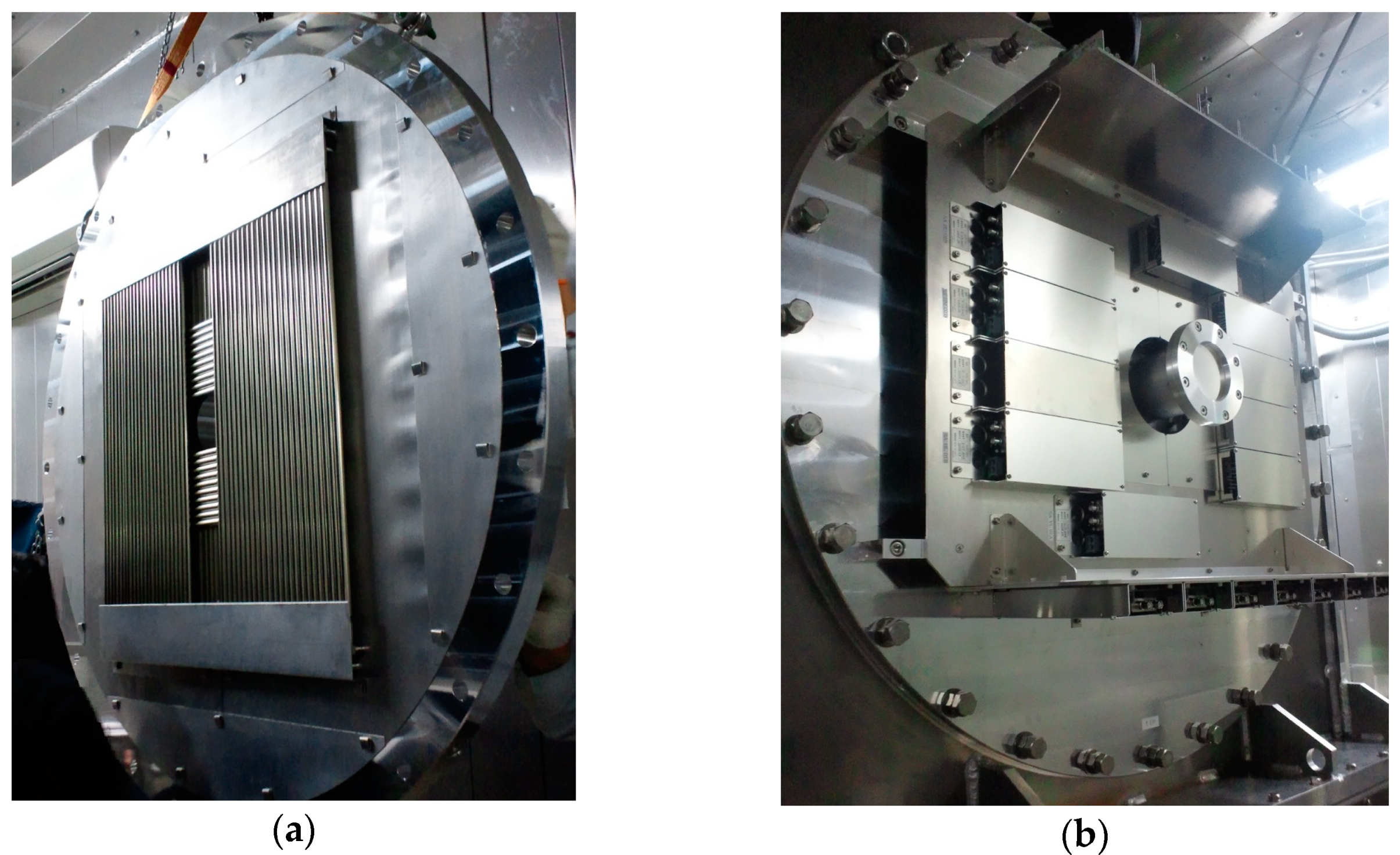
Figure 5.
Schematic picture of charge-division method.

Figure 6.
Scheme of event-mode data histogramming.

Figure 7.
Two-dimensional distribution of scattered neutron counts on the area detector (real-space histogram), which was covered with the cadmium mask plate. The calibrated correction factors (ai, bi, and ci) were applied at the data processing. The pixel color indicates the neutron count rate, with red as maximum and blue as minimum. The red, purple, and blue arrows indicate the positions of the cadmium mask strips for the first, second, and third layer PSDs, respectively. The white dashed circles indicate other cadmium pieces placed asymmetrically in order to check the overall PSD orientation.

Figure 8.
Neutron count efficiency along a typical PSD tube.
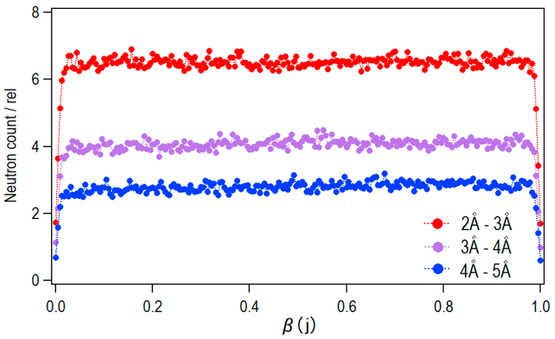
Figure 9.
SANS profiles of vanadium (t = 0.807 cm) (a) and glassy carbon standard (t = 0.116 cm) (b).
Figure 9.
SANS profiles of vanadium (t = 0.807 cm) (a) and glassy carbon standard (t = 0.116 cm) (b).


Table 1.
3He PSD tube lengths.
| Product Code | Effective Length [mm] | Inter-Axis Distance [mm] |
|---|---|---|
| E6867-600 | 600 | 749 |
| E6867-127 | 127 | 230 |
| E6867-100 | 100 | 203 |
Table 2.
Specification of the SANS detector on iMATERIA.
| Detector Area (SA bank) | 689 mm × 600 mm 91 mm × 91 mm (Central hole) |
| Number of PSD tubes | 46 (E6867-600) 14 (E6867-127) 20 (E6867-100) |
| Scattering angle, 2θ | 0.6°–5.5° (SA bank) 12°–40° (LA bank) |
| Moderator-to-sample distance | 26.500 m |
| Sample-to-detector distance | 4.684 m (first layer) 4.6695 m (second layer) 4.655 m (third layer) |
| Neutron wavelength range | 1–5 Å (single frame mode) 1–10 Å (double frame mode) |
| Standard collimation | 20 × 20 mm (2.17 m away from sample) 10 × 10 mm (0.22 m away from sample) |
| Total q range (double frame mode) | 0.007–0.60 Å−1 (SA bank) 0.13–4.3 Å−1 (LA bank) |
© 2020 by the authors. Licensee MDPI, Basel, Switzerland. This article is an open access article distributed under the terms and conditions of the Creative Commons Attribution (CC BY) license (http://creativecommons.org/licenses/by/4.0/).
Share and Cite
MDPI and ACS Style
Noda, Y.; Izunome, H.; Maeda, T.; Inada, T.; Ueda, S.; Koizumi, S. The Large-Area Detector for Small-Angle Neutron Scattering on iMATERIA at J-PARC. Quantum Beam Sci. 2020, 4, 32. https://0-doi-org.brum.beds.ac.uk/10.3390/qubs4040032
AMA Style
Noda Y, Izunome H, Maeda T, Inada T, Ueda S, Koizumi S. The Large-Area Detector for Small-Angle Neutron Scattering on iMATERIA at J-PARC. Quantum Beam Science. 2020; 4(4):32. https://0-doi-org.brum.beds.ac.uk/10.3390/qubs4040032
Chicago/Turabian StyleNoda, Yohei, Hideki Izunome, Tomoki Maeda, Takumi Inada, Satoru Ueda, and Satoshi Koizumi. 2020. "The Large-Area Detector for Small-Angle Neutron Scattering on iMATERIA at J-PARC" Quantum Beam Science 4, no. 4: 32. https://0-doi-org.brum.beds.ac.uk/10.3390/qubs4040032