Modeling Exposure to Heat Stress with a Simple Urban Model
by
 , ,
, ,
Peter Hoffmann
1,3,* ,
,
Jana Fischereit
2,3,
Stefan Heitmann
1,4,
K. Heinke Schlünzen
2,3 and
Ingenuin Gasser
1,4 1
Department of Mathematics, Universität Hamburg, Bundesstr. 55, 20146 Hamburg, Germany
2
Meteorological Institute, Universität Hamburg, Bundesstr. 55, 20146 Hamburg, Germany
3
Centrum für Erdsystemforschung und Nachhaltigkeit (CEN), Universität Hamburg, Bundesstr. 55, 20146 Hamburg, Germany
4
Lothar Collatz Center for Computing in Science, Universität Hamburg, Bundesstr. 55, 20146 Hamburg, Germany
*
Author to whom correspondence should be addressed.
Urban Sci. 2018, 2(1), 9; https://0-doi-org.brum.beds.ac.uk/10.3390/urbansci2010009
Submission received: 30 November 2017
/
Revised: 3 January 2018
/
Accepted: 16 January 2018
/
Published: 24 January 2018
(This article belongs to the Special Issue Environmental Impacts on Urban Health and Well-Being—Sectoral Components towards Understanding the Urban System)
Abstract
:As a first step in modeling health-related urban well-being (UrbWellth), a mathematical model is constructed that dynamically simulates heat stress exposure of commuters in an idealized city. This is done by coupling the Simple Urban Radiation Model (SURM), which computes the mean radiant temperature (), with a newly developed multi-class multi-mode traffic model. Simulation results with parameters chosen for the city of Hamburg for a hot summer day show that commuters are potentially most exposed to heat stress in the early afternoon when has its maximum. Varying the morphology with respect to street width and building height shows that a more compact city configuration reduces and therefore the exposure to heat stress. The impact resulting from changes in the city structure on traffic is simulated to determine the time spent outside during the commute. While the time in traffic jams increases for compact cities, the total commuting time decreases due to shorter distances between home and work place. Concerning adaptation measures, it is shown that increases in the albedo of the urban surfaces lead to an increase in daytime heat stress. Dramatic increases in heat stress exposure are found when both, wall and street albedo, are increased.
1. Introduction
Modeling the health of urban dwellers is a complex task. Urban areas affect human health due to the combination of multiple environmental stressors such as heat stress [1], air pollution [2], and noise [3]. All of these environmental stressors have elevated levels compared to their rural surroundings [4,5,6]. However, there are several factors that affect the impact of such stressors on health discussed by von Szombathely et al. [7] in their conceptual model for health-related urban well-being (UrbWellth). For instance, environmental stressors can only lead to a higher mortality or morbidity if urban dwellers are exposed to them (e.g., being outside). The exposure depends on the location of the urban dwellers as well as on their behavior [8] (e.g., activity patterns and choice of traffic mode) and on the intensity of the stressors. This intensity depends on the characteristics of cities (e.g., morphology, materials used, and green spaces) and consumer behavior (e.g., energy usage, emissions of pollutants from car traffic). It is therefore important for the modeling of UrbWellth to take into account different processes within the urban system, in particular human behavior.
Most studies assessing exposure to environmental stressors are either based on static population data [9,10] or require actual measurements [11]. There are, however, efforts to model individual behavior and combine this with stressor data using agent-based models [12]. This approach has not been feasible for a city with a large number of urban dwellers up to now because of computing constraints and lack of information about individual behavior. Thus, exposure modeling approaches with intermediate complexity are needed, where the modeling of urban stressors and a simplified representation of the movement of urban dwellers within the city are combined. Schindler and Caruso [13] did this by coupling multiple models (e.g., air pollution dispersion model, and traffic model) for an idealized city. With this coupled modeling system, they were able to identify urban morphologies that reduce the overall exposure to air pollution.
In this study, we focus on modeling exposure of commuters to heat stress. Heat stress is shown to increase the morbidity as well as mortality of humans [14]. Under heat wave conditions, mortality is increased during and shortly after such an event [1]. Thorsson et al. [15] showed that the mean radiant temperature is an appropriate measure for analyzing the heat stress related mortality of urban dwellers. depends on the morphology of the surrounding area, which can be quite heterogeneous within one urban area. It has been shown that an increase in the aspect ratio of street canyons (i.e., building height divided by street width) leads to a reduction of due to increased shading [16]. Hence, planning cities with narrow streets and high buildings might reduce heat stress exposure. However, it is not clear up to now how large this effect is during the course of the day and integrated over an entire city, because street orientation determines when shading is effective. Higher aspect ratios in average reduce wind speeds within a street canyon which would increase the heat perceived by humans assuming the same temperatures and . The intensity of this effect compared to shading is unclear in detail, but it is probably the smaller one and will not be included in the current investigations to keep them more simple.
Changing the morphology of the city has implications on the population distribution and subsequently on commuting patterns. The albedo of urban surfaces also has a large impact on the radiation within street canyons and consequently on . Since a reduced albedo is shown to decrease the urban heat island effect, urban planners are considering to the use of light colors as a climate adaptation measure. Schrijvers et al. [16] found that an increase in the albedo results in a increase. However, they also concluded that this effect is smaller than the effect of shading due to buildings. Consequently, a detailed investigation of the combined impact of changes in the aspect ratio and in the albedo on heat stress exposure is needed.
Taking an approach similar to Schindler and Caruso [13], we use a simplified coupled model in order to investigate the impact of different urban morphologies (e.g., building height distribution and street canyon geometry) and different surface characteristics (i.e., albedo) on the heat stress exposure of urban dwellers. In this model, a circular city is assumed with only two traffic flow directions, towards the city center and away from the city center. By introducing a multi-class multi-modal macroscopic traffic model the location of the commuters can be simulated depending on their home location, work place and choice of traffic mode. The heat stress is determined as a function of the city morphology and the albedo of urban surfaces with the Simple Urban Radiation Model (SURM) [17]. The dimensions and other simplified characteristics (e.g., building height distribution) of the city are based on data for the city of Hamburg because it has been extensively investigated within the interdisciplinary UrbMod project, which aims to develop a modeling framework for UrbWellth [7]. Hamburg is the biggest city in northern Germany with approximately 1.8 million inhabitants. Its climate is of marine influence: the winters are mild; while summers are moderately warm due to the moderating influence of the North Sea [18]. Despite the moderate summer climate, hot days (maximum temperatures ≥ 30 ) occur on average five days per year [19], which can cause daytime heat stress. Hence, meteorological conditions for a hot summer day are selected for the simulations in the present study.
The benefits of this simplified modeling approach are: (i) The effects of individual processes (e.g., impact of traffic on exposure) can be identified more easily than in a complex model; (ii) Computational effort is reduced, which enables production of a larger number of simulations. In addition, not enough information is available for more detailed simulations, especially with respect to individual behavior.
In Section 2, the simplified city, the different model components and the computation of exposure are described. The results of simulations conducted for a cloudless summer day as well as the results of sensitivity studies with varied city morphology and albedo are presented in Section 3 and discussed in Section 4. Concluding remarks are given in Section 5.
2. Model
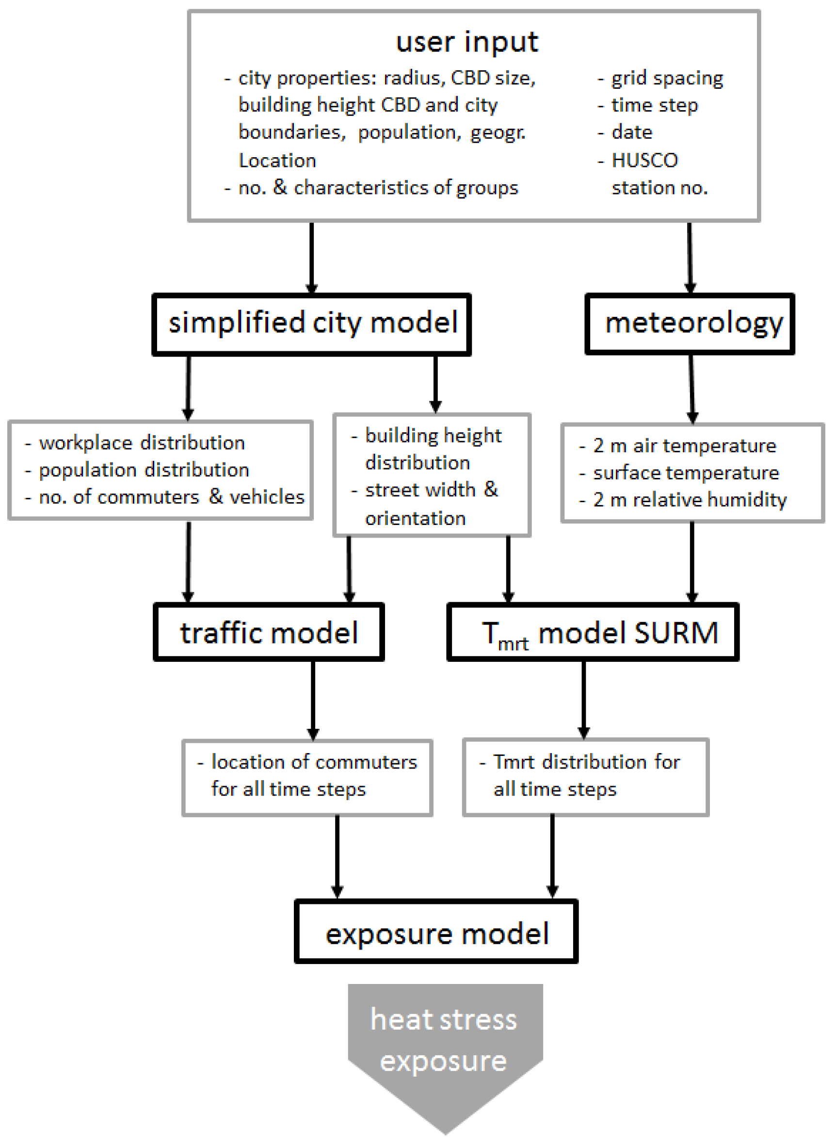
In the present study, we introduce a simplified model for heat stress exposure of commuters. Figure 1 shows the the different model components, their inputs and outputs, and the meteorological data employed. After all values are set in the user input routine, the simulation starts with setting up the simplified city (Section 2.1), which includes properties of the city (e.g., radius, geographic location, canyon geometries, wall and street albedo, working population), the model grid (e.g., grid length, street orientation increments), the groups (i.e., home and work location, and modal split) and the time steps for the model components. In the next step, the traffic model computes the location of the commuters throughout the day (Section 2.2). Thereafter, the meteorological data (Section 2.4) are imported in order to run the SURM model [17] (Section 2.3), which calculates the mean radiant temperature, , on the same grid and for the same time steps. Since and the traffic are currently coupled through the building height distribution of the city they can be run sequentially. It is, however, possible to run both modules in parallel if needed (e.g., if feedbacks are implemented). Finally, the exposure is computed for the different groups using a given threshold for (Section 2.5). A detailed description of the model components and data are given in the following sections.
2.1. Simplified City Model
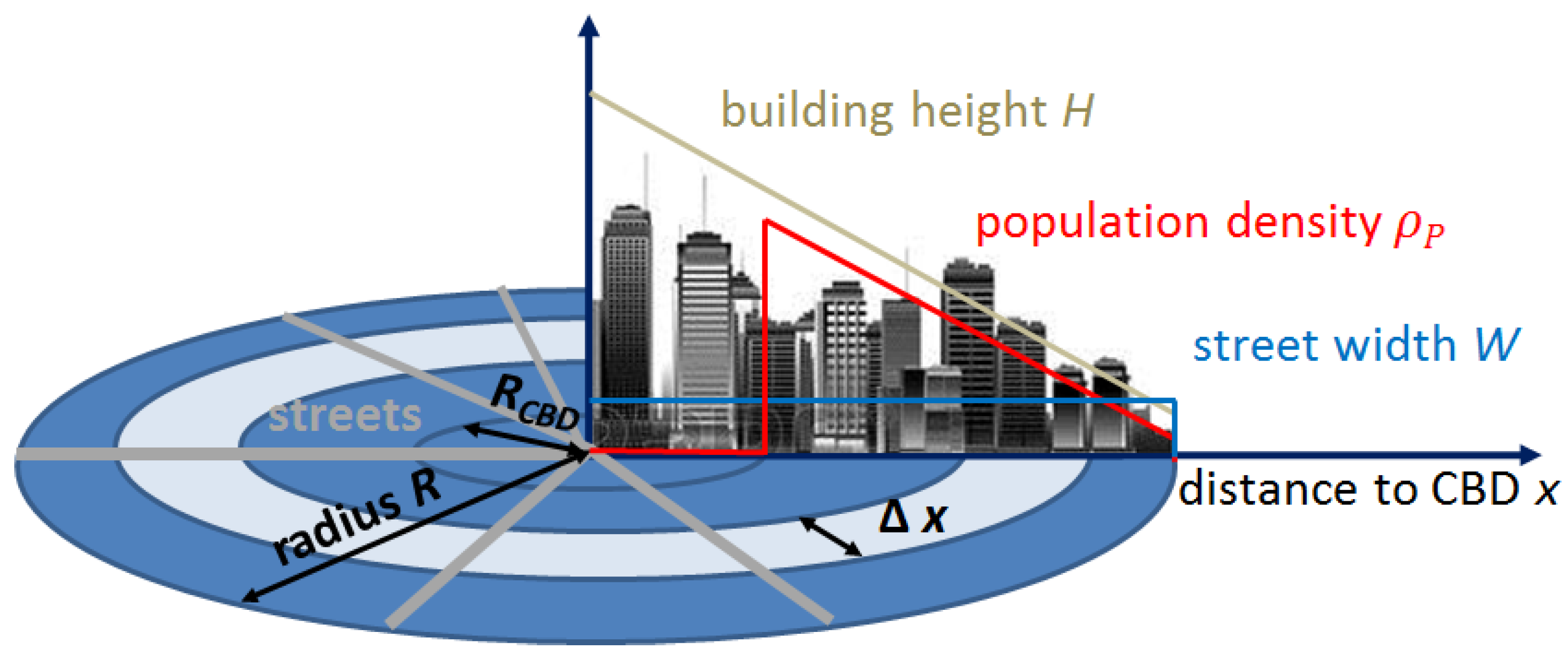
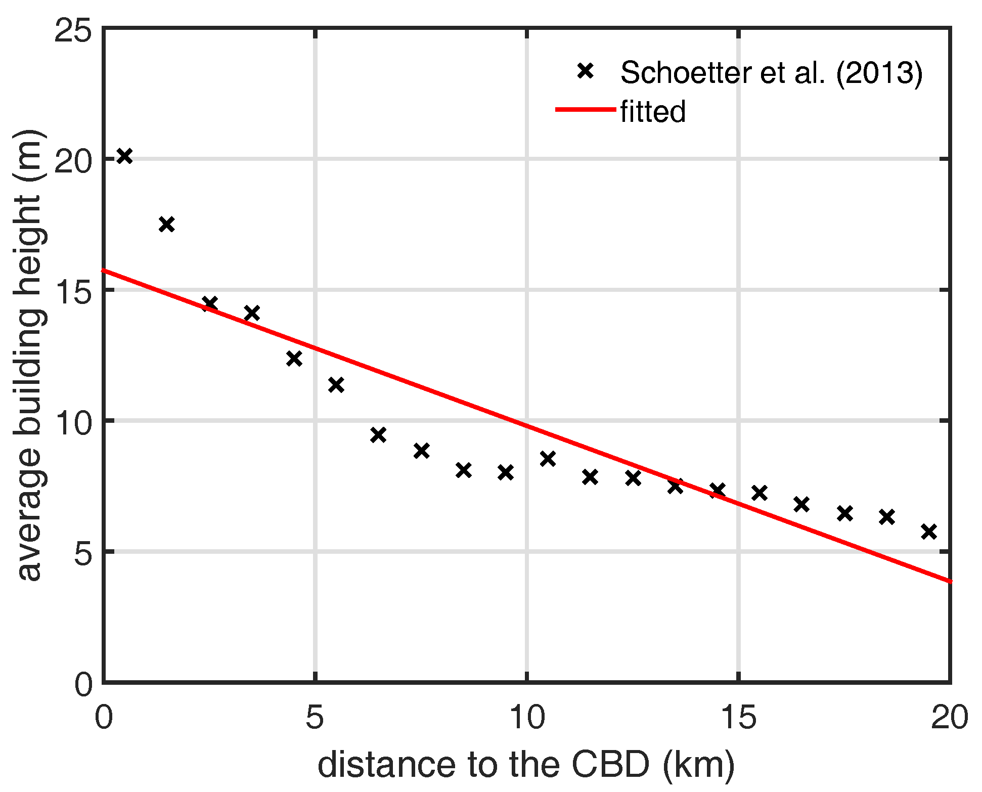
The simplified city used for the simulations is assumed to be circular with a radius R (Figure 2). It consists of a central business district (CBD) in the city center, where most of the workplaces are located, surrounded by mostly residential buildings. The height of the buildings H depends only on the (non-negative) distance to the CBD, x (Equation (1)). In this paper, a negative linear relationship is assumed: the further away from the CBD the smaller are the buildings. The factor is chosen so that H is equal to in the CBD and equal to at the city boundaries (Equation (2)). The idealizing assumption of a linear change of H can be justified with an analysis of building height data for Hamburg taken from Schoetter et al. [4]. Figure 3 shows the building height average for different distances from Hamburg’s city center using 1 km bins and the corresponding linear fit (explained variance = 0.78). Close to the city center building heights increase rapidly, which is on the one hand due to larger office and retail buildings near the city center and on the other hand due to the smaller area used to compute the average building height. The latter can lead to a large impact of single high buildings (e.g., Sankt-Petri-Church with a 132 m bell tower). This is also reflected in the large height variability within the distance bins (not shown). Hence, as a first order approximation, a linear dependency is reasonable.
The population density is assumed to be proportional to H and therefore also a function of x (Equation (3)), with the exception of the CBD. Within a radius , the population is set to zero assuming that the buildings are occupied by offices only. The constant is positive and needs to be calculated from city properties. The density needs to be multiplied with the area A in order to yield the population at a certain distance from the CBD.
The constant needs to fulfill the constraint that the integral over all circular rings equals the total population (Equation (4)). Since the population within the CBD is set to zero, the limits for the integral are the radius of the CBD, , and the radius of the city, R.
Solving the integral gives:
The average street width W is set to be constant throughout the city because there is no obvious functional relationship between street width and distance to the CBD. Hence, only the aspect ratio of the street canyons decreases linearly with x. is used to couple the city model with the module of the mean radiant temperature described in Section 2.3.
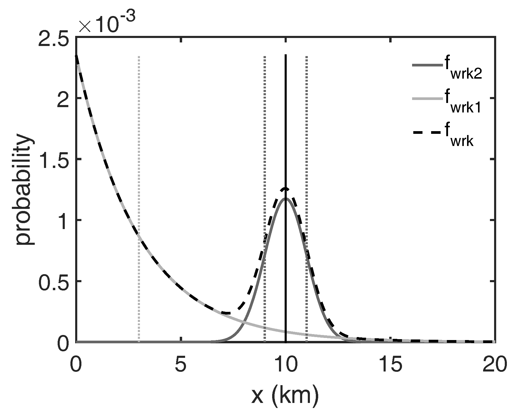
The spatial distribution of workplace of citizens has two modes for a given location (Equation (7)). The first mode, , reflects that most workplaces are located close to or in the CBD. It is approximated by an exponential distribution (Equation (8)) with an e-folding distance , which can be viewed as the size of the CBD. The second mode takes into account that there are workplaces close to the home location (e.g., people working in grocery stores or other service providers). Here, no directional preference is assumed. As a functional relationship the normal distribution is chosen (Equation (9)), where only the standard deviation needs to be specified. As an example, Figure 4 shows the two distributions as well as the combined distribution for urban dwellers living 10 km from the CBD.
For the simulations conducted in the present study, the city is discretized with equal grid spacing with respect to distance to the CDB, , and street orientation, .
The diversity of the behavior of the urban population population groups is introduced to the coupled model. These are groups that differ with respect to choice of traffic mode and working hours. The group properties could be extended using socio-demographic variables such as gender, age, income and preferred choice of home location. These variables could be determined from geospatial analysis in combination with surveys as done by Kandt et al. [20].
2.2. Traffic Model
The traffic model is needed in order to know the location of the commuters throughout the day because the heat stress exposure (, which varies throughout the city) depends on location. Therefore, the model should be able to track the location of individual vehicles or group of vehicles. There are at least two major approaches in modeling road traffic: macroscopic and microscopic. For the current problem, microscopic models, which simulate the movement of individual cars, are not feasible because it is too expensive to compute the traffic for the whole city due to the large number of cars. Instead a macroscopic model is applied, modified to track groups of vehicles in the simulations. Macroscopic models were introduced in the 1950s by Lighthill et al. [21] and describe the traffic flow using the macroscopic quantities vehicle density, , and average velocity, v. Using the conservation of the number of vehicles, , within a discrete area the flow can be modeled using the continuity equation (Equation (10)).
The number of vehicles can be expressed in terms of vehicle density in an area A (Equation (11)). The area A for the annuli of the circular city can be calculated using Equation (12).
The velocity v decreases, similar to Greenshields model, linearly with increasing until a maximum car density (used values in Table 1) is reached, where (Equation (14)).
Since we are interested in the exposure of different groups, with different home and work place locations as well as different choice of transport mode, needs to be split up into partial densities , where . Each describes the number of vehicles from a specific population group that has the same home and work location. The total number of densities is determined based on the number of grid points, , the number of flow directions, (=2; towards the CBD and away from the CBD), and the number of population groups, , using the following formula:
Using the -vector, Equation (13) becomes:
while the velocity is dependent on the total density at each grid point (Equation (17)).
Zhang et al. [22] showed that the flow-density relations of bicycle and car traffic are similar when the maximum density and the maximum velocity are chosen accordingly. Therefore, Equations (16) and (17) are used to model the bicycle traffic in the present traffic model. Modeling public transport (buses, subways, and rapid-transit trains) is not as easy to implement in a simple model, as introduced here. However, most public transport is climatized and some trains run underground. Therefore, public transport is not considered in the present study but will be included in the modeling system in the future following the approach of Gasser et al. [23]. In the current version of the traffic model the information about whether the commuters are on the road or either at work or at home is added. This is achieved by introducing an indicator function, (Equation (18)), that depends on the time t as well as on the location x. can take the value 0 for not being on the road and +/−1 for being on the road. The sign of indicates the flow direction. and denote the place of work and home, respectively. and are the times when commuters start to go to work and to go home, respectively. is equal to the end of work while is computed for each separately so that the the commuters arrive at work on time, assuming no traffic jams. depends on the mode of transport, the distance to work, and the start of work. (=12:00 CET) and (=24:00 CET) are set to distinguish between commuting to work and from work.
This yields the final model equations:
Equations (17) and (20) are solved using a local Lax-Friedrich scheme (LLxF) [24], with constant grid spacing . The latter is chosen because it accounts for a rarefraction wave, which occurs when gets close to and therefore v close to 0 km/h (i.e., traffic jam). Special care needs to be taken at the boundaries of the city in order to conserve the total number of cars. Hence, an extra grid point is added at both ends of the grid. At these grid points is set to 0.
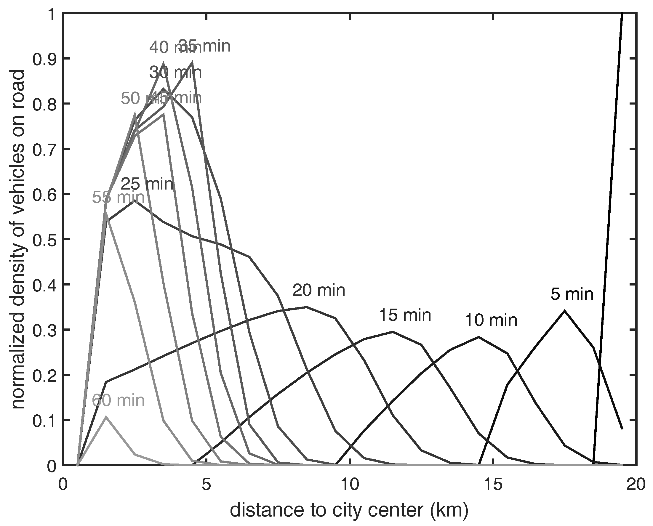
To test the applicability of the LLxf scheme to the given problem, test simulations are conducted with . The simulation starts ( min) with at the last grid point ( km) and for all other grid points. The maximum velocity is set to 50 km/h, the grid spacing to 1 km, the time step to 1 min and the flow is directed towards the city center. Figure 5 presents the simulation results normalized with for every 5th time step. The use of the LLxF scheme leads to a rarefraction of the density within the first time steps, which reflects the start of vehicles in front of a traffic jam. The normalized density increases after 15 min due to the decrease of the area with decreasing distance to the CBD. After about 20 min, the first vehicles reach their destination (i.e., CBD). Thereafter, the density increases near the CBD . Due to the large number of vehicles, the velocity decreases. This results in a traffic jam and a backwards moving shock wave, which is visible between 25 min and 35 min. Here, the density increases rapidly to 90% of while the density peak moves into the opposite direction (away from the CBD) compared to the traffic flow direction (towards the CBD). This is a typical behavior of traffic flow [25]. After 40 min the rate of vehicles arriving at the CBD becomes larger than the rate of vehicles approaching the traffic jam. Consequently, the density decreases until all vehicles have arrived at the CBD after around 65 min. Based on these results it can be concluded that the traffic model in combination with the LLxf scheme produces a realistic traffic flow.
2.3. Model
As a measure for heat stress, the mean radiant temperature is used, because it is a good measure for human comfort [15] and is very closely linked to the urban morphology [26,27]. is defined as the uniform temperature of an assumed black-body radiation enclosure in which a subject would experience the same net-radiation energy exchange as in the actual more complex radiation environment [28]. can be calculated according to Equation (21):
Here, denote long-wave radiation fluxes and diffuse radiation fluxes from various sources with different view factors . represents the direct shortwave radiation flux reaching the human body that is assumed to have albedo and emissivity and projection factor . is the Stefan-Boltzmann constant. In this study, the Simple Urban Radiation Model (SURM) [17] is applied to estimate the radiation fluxes within an idealized symmetrical street canyon of infinite length without vegetation on a cloudless day. The model simulates incoming shortwave radiation based on the day of the year and geographical latitude and accounts for the absorption of radiation by water vapor in the atmosphere. Based on aspect ratio , street orientation and time of the day, shading of the street canyon floor, walls and the person are calculated. The diffuse radiation fluxes from the sky and the reflected radiation fluxes from walls and ground are treated as lambert equivalent; long-wave radiation fluxes from sky, walls and ground are considered as diffuse isotropic. In the model version (2.2) of SURM applied in this paper, surface temperatures of shaded walls and ground areas are assumed to be equal to air temperature. For sunny areas a uniform but time dependent wall and ground temperature is prescribed (Section 2.4). A detailed description of the model is given by Fischereit [17].
The applied accounts for rotational symmetric people standing within a street canyon and not for car passengers. The heat stress within a car depends on many different aspects, for instance if the car is air conditioned or not and how fast the car is going. There are comprehensive models for heat stress in vehicles available [29]. It is planned to include such models in the modeling framework in the future. For the present study, the computed can be regarded as a measure of potential heat stress of car passengers, because radiation is an important factor when determining heat stress within cars.
2.4. Meteorology
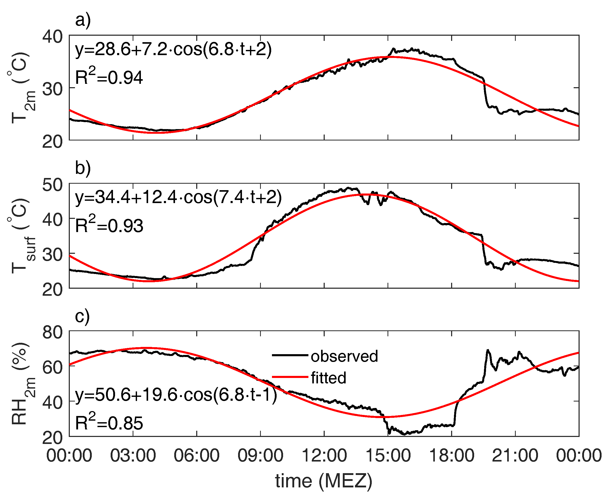
The meteorological data of the Hamburg Urban Soil Climate Observatory (HUSCO) [30] are used as input data for calculations (Section 2.3). HUSCO provides measurements for every minute from several stations within the city of Hamburg. The observations of 2m temperature, , surface temperature, , and 2m relative humidity, , at the CBD station “Innenhof Stadthausbrücke” for a summer day with extreme temperatures (4 July 2015; Figure 6) are selected for the simulations conducted in this study. Here, it is assumed that the meteorological conditions, consisting of temperature, humidity and wind, do not vary throughout the city, neglecting for simplicity the differences that are found in real urban areas with complex impacts of urban structures e.g., [18,30]. These simplifications are a first essential step for assessing the feasibility of a joint modeling of morphology and and traffic. The surface temperatures as well as the wall temperatures are set to in the sun and are assumed to be equal to in shade. By doing so, we account for the most important spatial variations during daytime e.g., [31] and therefore the effect of morphology on radiation, if homogeneous surface properties and calm wind conditions are assumed. This simplifies the complex relationship between the urban materials and structures found within cities with heterogeneous surface properties e.g., [32]. To reduce the noise, the meteorological data are fitted to a trigonometric function (Equation (22)) using the Levenberg-Marquardt nonlinear least squares algorithm [33].
Here, t is the time in seconds starting at midnight with . The fitted functions and the explained variance of the fits are shown in Figure 6. For both and , the observations can be sufficiently well reproduced indicated by a of 0.94 and 0.93, respectively. The performance of the fitted time series is not as good () but still satisfactory. It reproduces the observed time series until 14:00 CET quite well. Thereafter, rapid changes in occur, which cannot be captured with a single frequency . However, the errors are in an acceptable range of +/− 10%. These functions are used as the idealized meteorological forcing, assuming zero wind conditions.
2.5. Exposure Model
The exposure to an environmental stressor such as heat stress due to high temperatures, , is the sum of the exposure at the workplace, , the exposure during the travel to work, , the exposure at home, and the exposure during free time . The current version of the model does not allow the computation of the exposure at home and at work because heat stress, i.e., , in buildings is not accounted for. There are detailed models for heat stress in buildings available [34]. It is planned to include such models in the future. In addition, the computation of is quite difficult because of the lack of knowledge and corresponding data about the behavior and therefore the location of urban dwellers during their free time. Hence, the focus of this study is on the exposure during the commute to work .
Thorsson et al. [15] showed that only the exposure to above (heat stress) and below (cold stress) a certain threshold can be related to a higher mortality rate. In the present study the focus is on heat stress. Hence, following Lau et al. [35] the exceedance of for heat stress is used to calculate the exposure (Equation (23)). They introduced a variable called overheating degree hours (), which is the sum of time with values above . It can be generally written as:
where is the time interval of interest (e.g., years or days). Lau et al. [35] did not explicitly consider the exposure of the population. The latter is represented by utilizing the traffic model (Section 2.2). With this model, it is possible to compute the exposure for every subpopulation (i.e., partial densities in the traffic model) because their position is known throughout the day. The average exposure over a day can then be computed with the following equation:
where c is . It is also possible to calculate the exposure of certain groups (e.g., only bike commuters) when only the results for the corresponding are summed up and is replaced by the corresponding population group. In addition, the exposure can be computed as a function of distance by changing the limits of the spatial integral accordingly.
3. Simulations
3.1. General Set-Up
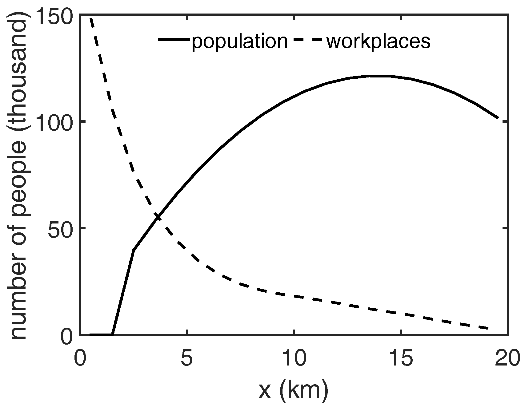
For the first test of the coupled model, the population is split up into four groups (Table 2), which each make up 25% of the commuting population. The first two groups work 8 h a day (typical for German workers), but with different working hours. For both groups, a half an hour lunch break is included. The modal split for commuters in Hamburg is 41% cars, 33% public transport, 11% bikes, and 12% other [36]. In the present study, only car and bike traffic are considered. Hence, the modal split for the groups is chosen to have an average ratio of cars to bikes of 4 to 1. Group 1 uses more bikes and fewer cars to commute to work compared to the average commuter, while, for Group 2 it is vice versa. The other two groups have the same modal split as the first ones but work only part time. The ratio between part-time and full-time workers is 0.37 following data from the city of Hamburg. The population and workplace distribution for the simplified city are given in Figure 7. About 50% of all workplaces are located within 3 km from the CDB while more than 2/3 of the urban dwellers live further than 10 km from the CBD.
3.2. Reference Case
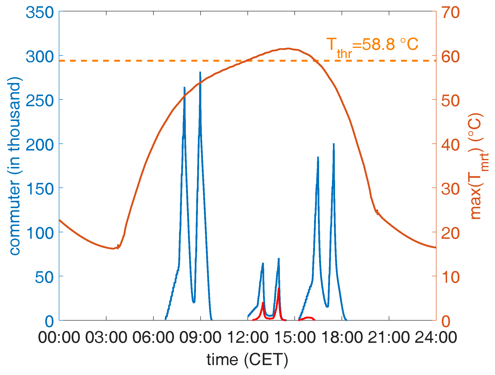
The results for the simulations using a building height of 16 m in the CBD, based on the fitted curve in Figure 3, are presented in Figure 8. This figure shows the time series of the maximum in the city, , the total traffic (cars and bikes), and the exposed commuters. The diurnal cycle of is asymmetric and skewed towards the afternoon, which is due to the combined effect of the solar radiation and the meteorological variables (Figure 6). The phase of both and is shifted towards the afternoon, while the effect of the solar radiation is symmetric with respect to solar noon (not shown). Consequently, increases rapidly after sunrise but slows down after 7:30 CET, when the increase is mainly due to the increase in and . is reached at 12:00 CET while the maximum of 61.6 is reached at 14:30 CET. Thereafter, decreases at a rate that is comparable to the increases in the morning hours. Hence, is crossed at 16:15 CET only 1 h and 45 min after the maximum.
The number of commuters on the road is not a continuous variable because only the traffic of commuters with regular working hours (start of work in the morning and end of work afternoon or early afternoon) is considered. Hence, there are two pronounced peaks in the number of commuters on the road shortly before 8:00 CET and 9:00 CET in the morning and two smaller peaks in the early afternoon (around 13:00 CET and 14:00 CET), which correspond to part-time workers driving home, and two peaks in the late afternoon (17:00 CET and 18:00 CET). Since values above occur after 9:00 CET and before 16:30 CET mostly part-time worker coming back from work are exposed to heat stress. Only a small fraction of commuters with longer working hours are exposed. This is reflected in the average values for for the four groups. Group 4 ( = 5.5 min per commuter) is exposed the most, followed by Group 3 ( = 3.7 min per commuter). Group 1 ( = 0.5 min per commuter) is only marginally exposed while Group 2 shows nearly zero exposure. Since bike commuters need longer to go to work they are more exposed than car commuters.
3.3. Influence of City Structure
To investigate the impact of the urban morphology on heat stress exposure, simulations with different building height distributions () and different street widths () are conducted. The building heights influence both the aspect ratio and the population distribution and therefore and traffic, respectively. The only model parameter that is chosen to vary is the building height in the CBD , which affects the building height, home location and work place distribution. The street width W only has an impact on and therefore on . As a measure of traffic the accumulated time spent on the road and in a traffic jam ( 15 km/h for cars and 5 km/h for bikes) is computed.
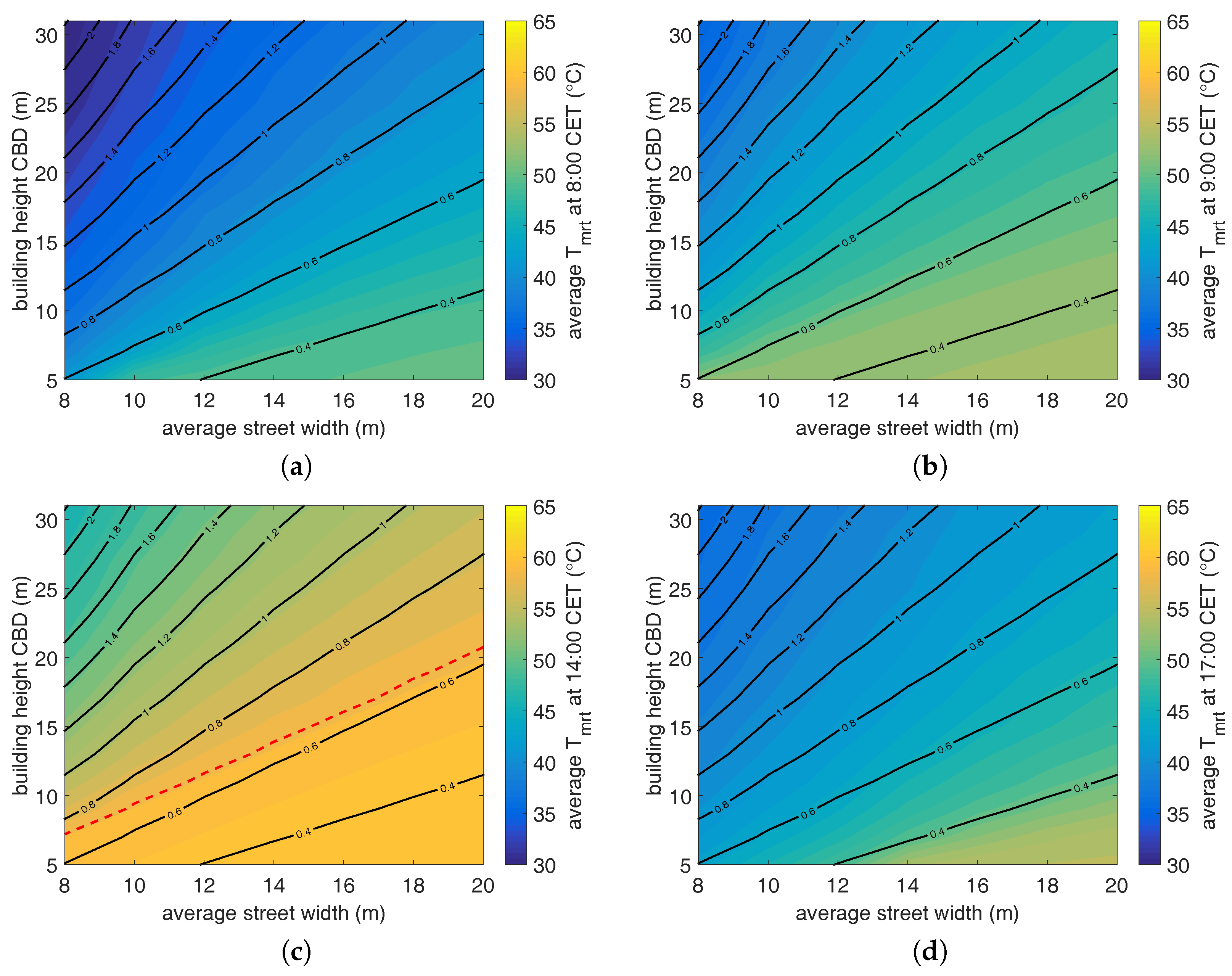
The impact of the different city morphologies on the is presented in Figure 9. In general, the area averaged for the whole city increases with decreasing building height and increasing W during daytime. The influence of the two variables, however, depends on the time of the day. At 9:00 CET (Figure 9b) and 14:00 CET (Figure 9c) both variables are equally important because the contour lines are almost aligned with the contour lines of the averaged . For average of 0.6 and lower a saturation of the at 14:00 CET is reached. Due to the large zenith angle and the large distances between buildings the influence of the buildings on the radiation budget diminishes and the reaches the value for a human on an infinite plane. The closer the time is to sunrise and sunset, respectively, the more important W becomes, as indicated by the crossing of and contour lines (Figure 9a,b,d).
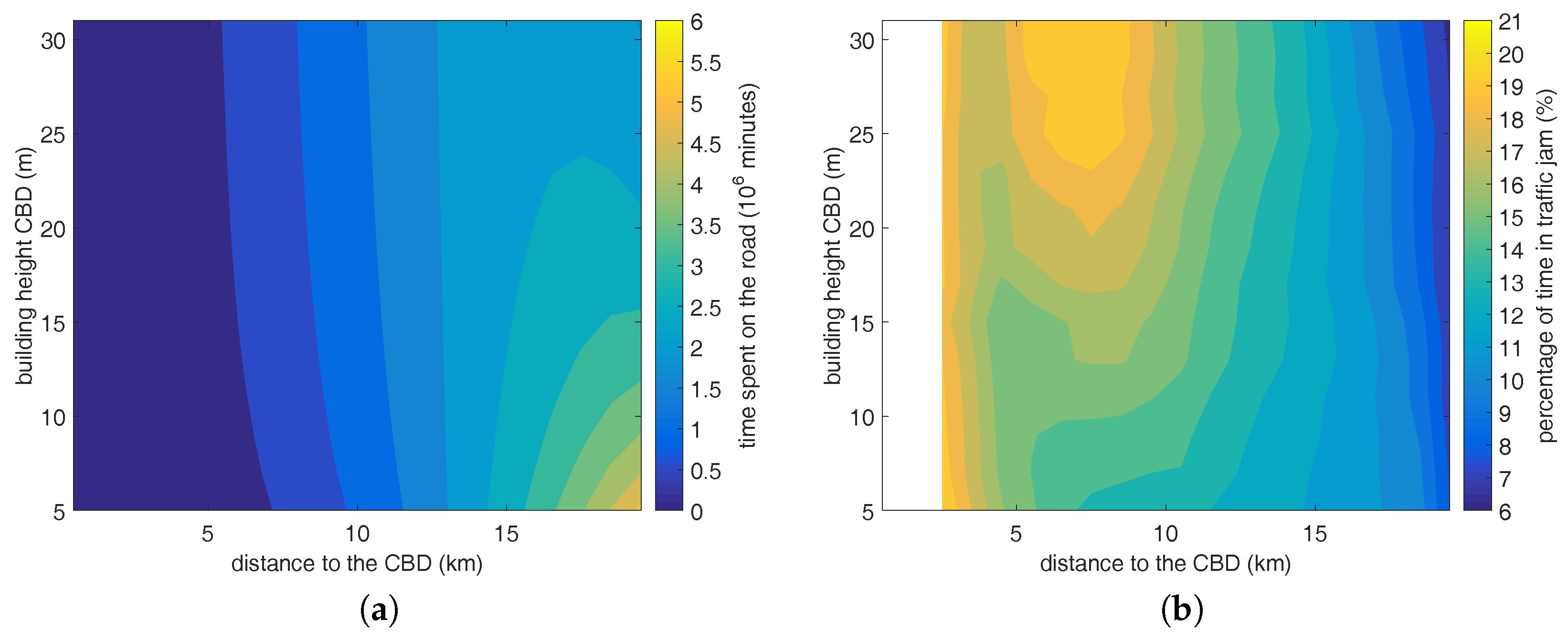
In Figure 10, the dependency of the building height distribution (i.e., population distribution) on the traffic is presented. Figure 10a shows the total time spent on the road for the different home locations. A more compact city structure (i.e., large ) leads to a reduction in the total time spent in traffic. For = 5 m the total time is min (33 min per commuter), while for = 31 m it is only min (27 min per commuter). This is mainly a result of urban dwellers living closer to the CBD. The increase in traffic jams for more compact city structures slightly compensates for this effect. Figure 10b shows the percentage of time spent in a traffic jam as a function of and the distance of the home location to the CBD. The increase in traffic jams of more than 23% at a distance of 5 and 9 km from the CBD can be attributed to the car traffic. Traffic jams of commuters riding their bike are rare in the simulations conducted but the commuting time still increases because of Equation (19). Traffic jams increase the commuting time up to 31% when only car traffic is considered.
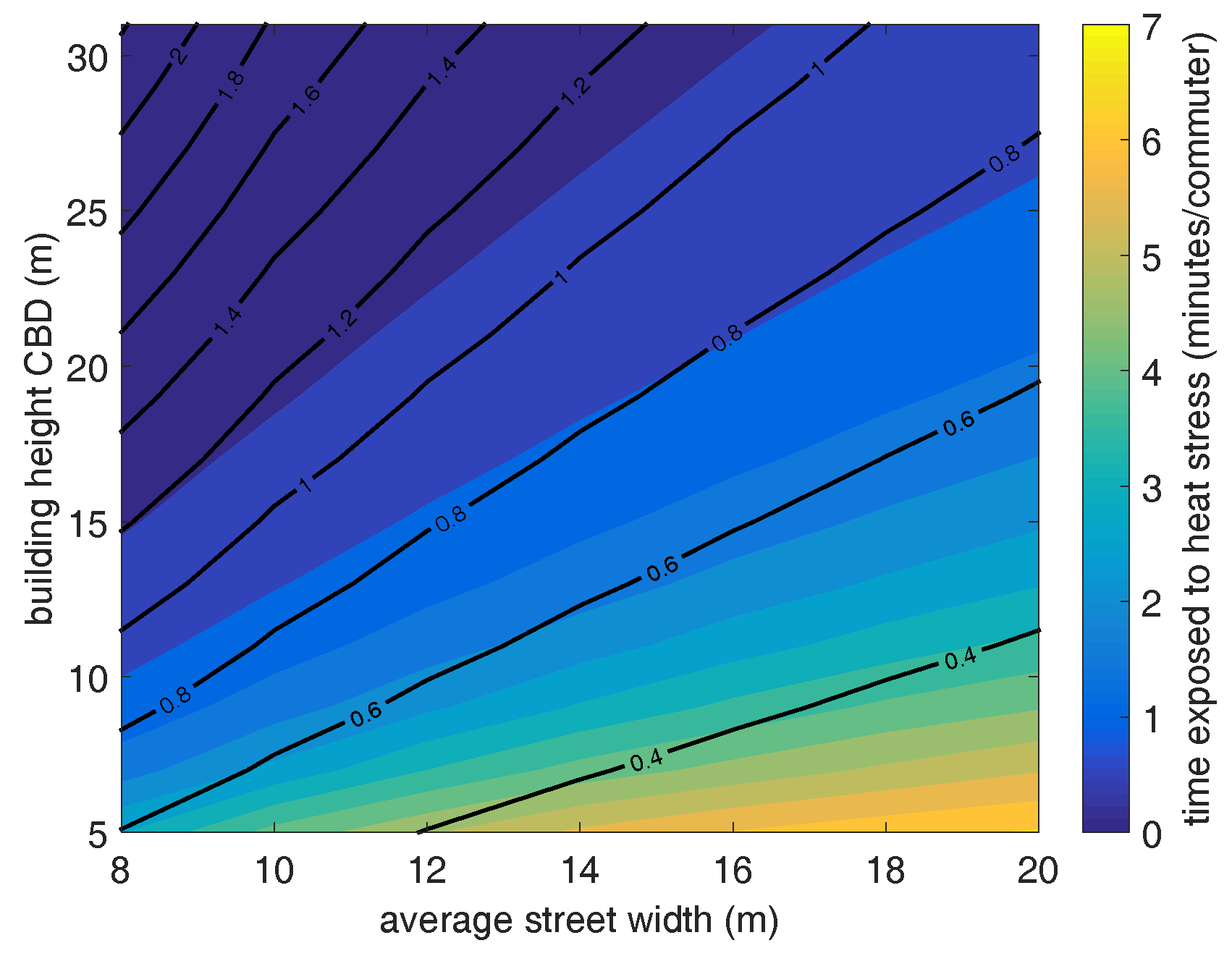
Figure 11 shows the average exposure for all commuters as a function of and W. The lowest values are associated with large values. While for large values is closely related to , becomes more and more independent of W for small values. This can be explained by the increasing influence of the time spent outside with decreasing compared to the influence of the morphology on in the early afternoon (Figure 9c), with changes of and being aligned.
3.4. Influence of Albedo
Another climate adaptation measure that can be investigated with the simple coupled model is the modification of urban materials with respect to their albedo (e.g., painting walls and roofs of buildings white). is a measure for the reflectivity of the surfaces with respect to radiation. The larger , the more shortwave radiation is reflected, which could lead to a reduction of the air temperature. For that reason, it is proposed to use materials with higher for climate adaptation. Within the model it is possible to vary the values of for walls and street surfaces, and , respectively. In the first step, only the values for are changed and in the second step, is also changed. The range of values (0.1 to 0.6) is taken from Boettcher et al. [37], who implemented adaptation measures developed for the city of Hamburg in an atmospheric model. An of 0.6 can be reach by using white or by using more reflective walkways [37].
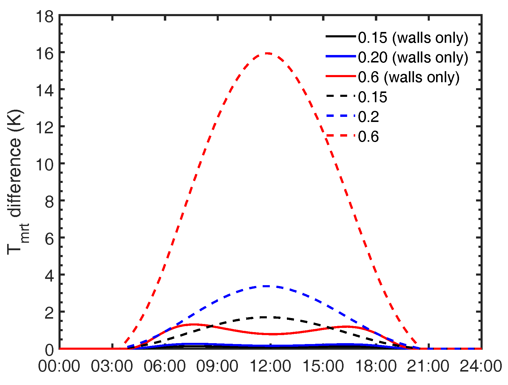
Figure 12 shows the time series for the difference in the averaged compared to the simulation with (all other variables correspond to the reference case). The impact of changing (solid lines in Figure 12) is small compared to changing the albedo of all surfaces (dashed lines in Figure 12). The increase of from 0.1 to 0.6 results in increased values of up to 1.3 K in the early morning and late afternoon hours and up to 0.8 K around noon. Smaller changes in (e.g., from 0.1 to 0.2) show increases that are negligible. The diurnal behavior can be explained by the small solar angle around sunrise and sunset, which results in a larger influence of the reflected radiation of the walls in the radiation budget. Increasing of all surfaces leads to much larger increases that follow the curve of the incoming solar radiation (not shown). Even a small change in from 0.1 to 0.15 increases the averaged by up to 1.7 K around noon. An increase from 0.1 to 0.6 results in a dramatic increase of almost 16 K around noon. The increases in in both sensitivity studies affect also the exposure of the urban dwellers to heat stress. Changing from 0.1 to 0.6 results in an increase in of about 104% (from 1.3 min per commuter to 2.7 min per commuter) while the same change in of all surfaces results in an that is more than 90 times larger (from 0.16 min per commuter to 14.8 min per commuter).
The results for the different groups (Table 2) as well as car and bike commuters are given is Table 3. When changing only , all groups show approximately a doubling in , except for Group 2, which is almost not exposed at all. In addition, for car and bike commuters the relative change is quite similar. A different relation can be seen when changing both and . Group 4 experiences the largest absolute increase of +23 min per commuter. Since the other groups are almost not exposed when = = 0.1, the relative changes are quite large for these groups. For = = 0.6, even the full-time workers are exposed. In addition, the increase is larger for bike commuters than for car commuters.
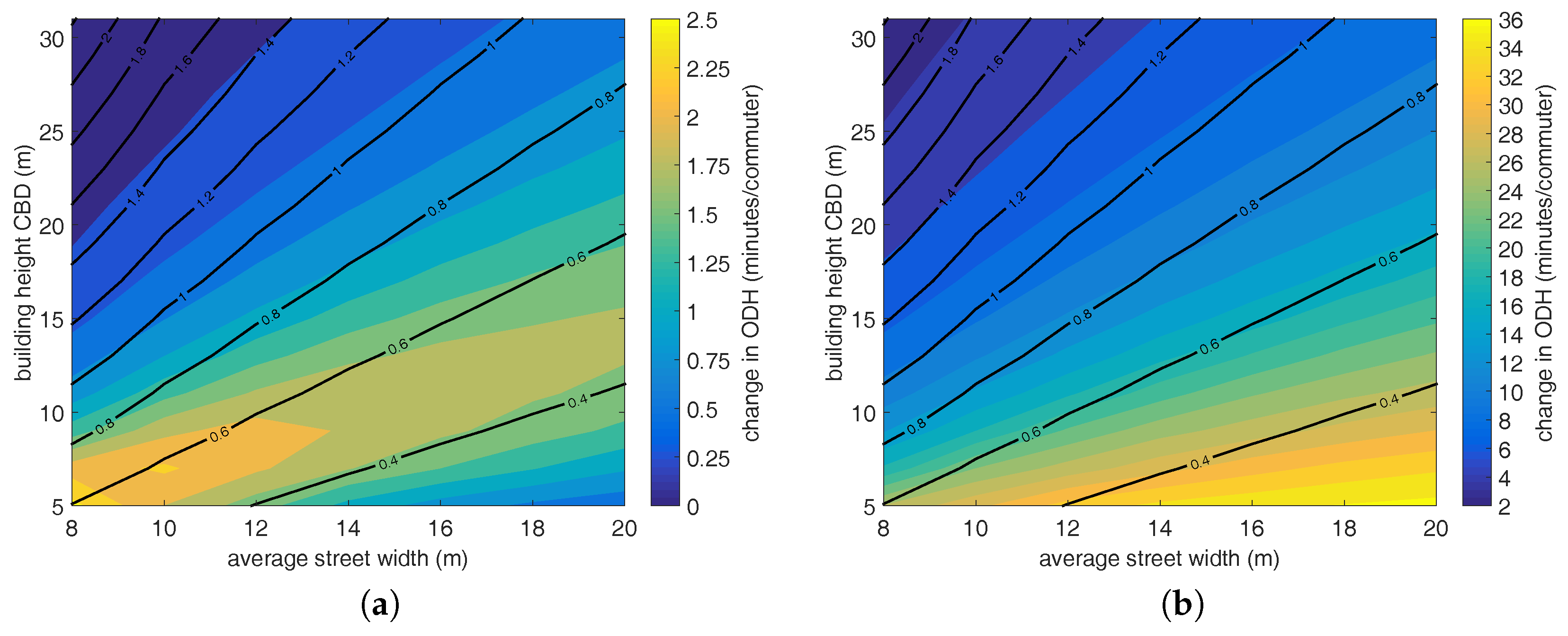
The combined effect of the changes and changes in the city morphology are presented in Figure 13. Here, the differences in are shown as a function of W and . For increased (Figure 13a), the differences in are closely related to the averaged . For both large and very small , the differences are small. A maximum increase of 2 min per commuter and more can be found for between approximately 0.5 and 0.7. The changes in are one magnitude larger if of all surfaces is increased (Figure 13b). The increases show a moderate functional relationship to , with a maximum increase of more than 30 min per commuter for < 0.4.
4. Discussion
Several assumptions were made for the development of the coupled model in order to reduce the complexity of the problem. The exposure of commuters to heat stress is modeled assuming simplified cities with idealized behavior of the population groups and idealized morphology. These assumptions were essential to solve the problem with reasonable computing time and data storage use. In addition, missing information (e.g., the relationship between work and home location or between city morphology and population distribution) currently makes very detailed models challenging.
Assuming a circular city neglects the heterogeneity of cities resulting from topography (e.g., valleys, mountains, rivers, and lakes) and from urban development, which might shift the CBD to a different location or leads to heterogeneous population density (e.g., if slopes are too steep for building). This heterogeneity does not allow the detection of the impact of single changes (e.g., building height) on heat stress due to the complex interactions between city morphology and traffic. Hence, the results for realistic cities (e.g., cities in narrow valleys or coastal cities) will differ in detail from these presented here. Nonetheless, some findings can be generalized for cities in the mid-latitudes. Since the diurnal cycle of is linked closely to the incoming solar radiation, the maximum will be around noon or in the early afternoon. Consequently, part-time workers with morning shifts or workers who work outdoors are more likely to be exposed to heat stress during heat waves (high temperature and clear sky) than office workers with longer working hours.
For a realistic city, the traffic is also much more complex than it is considered to be in the present study. Streets divert into a complex network, which includes streets with non-uniform average width and varying capacities (i.e., different maximum vehicle density), intersections, and traffic lights. Furthermore, only the traffic due to commuters is considered here as is done in other exposure studies e.g., [13]. Traffic due to public transport and heavy vehicles as well as non-work-related traffic is neglected. For the current problem this simplification does not have a large impact on the results because the increase in commuting time due to traffic jams is only up to 23% (Figure 13a). It is, however, possible that the travel time and time spent in a traffic jam (Figure 10) will be impacted by additional traffic. For exposure studies of traffic noise or traffic-induced air pollution these simplifications would have a much greater effect because stressor and traffic are closely related. The large uncertainty results from the unknown relationship between home location and workplace. In the present model configuration, the total commuting time is small for compact cities because more commuters live close to their workplaces.
Commuters using public transport or other means of transport are not considered in this study. Hence, the findings on heat stress exposure are only valid for commuters who use their car or bike. In order to include all commuters in an exposure model, additional assumptions about the time spent outside or on the heat conditions in trains and buses would have had to be made. This would have required data on how much time they spend to walk to the next public transportation station or to walk directly to work, which were not available. However, such data will be collected within the UrbMod project with the help of detailed surveys. In addition, the population distribution, which is varied in the present study by changing the building height distribution, is likely to have an effect on the modal split within a city. Again, additional information on the dynamics of this relationship is required to take it into account in the modeling system.
is regarded as a proxy for heat stress of urban commuters in this study. It is valid for commuters who use their bike because their body is exposed to the radiation within the street canyon. While more complex models for outdoor human comfort exist that in addition to the radiation budget account for the effects of wind speed, humidity, air temperature and even of clothing and physical activity [38,39] studies show that is a good measure for heat-related mortalities [15], which indicates that it sufficiently reflects the daytime heat. For the human comfort of car passengers more complex models exist [29]. However, they require a number of input data that need to be collected (e.g., geometry of the cars or availability of air conditioning) before such models can be applied to assess the heat stress for a large number of cars. Hence, having a simple measure such as that accounts for the radiation, which plays an important role in vehicular thermal comfort models, is a good first guess. Keeping in mind the limitations mentioned, the number of commuters exposed to heat stress might be overestimated using just as a measure for heat stress.
In addition, the model employed neglects shading of trees as well as evaporative cooling effects of urban green. Both effects could reduce the heat stress of commuters. Furthermore, by assuming a constant throughout the city the effects of hot urban surfaces such as asphalt or walls might be underestimated. The influence of the abovementioned effects on the heat stress should be considered by taking into account the spatial variability of the meteorological conditions using mesoscale e.g., [40] or building-resolving microscale atmospheric models e.g., [41].
Schrijvers et al. [16] also showed that an increase in the aspect ratio leads to a reduction of for large parts of the street canyon. However, they also simulated the effect of the mixing of the air within the street canyon, which has additional effects on the distribution near the surface. As a consequence in some parts of the street canyon could increase with increased aspect ratio under the right meteorological conditions. However, the case study for Hamburg by Schoetter et al. [4] also showed that the perceived temperature (PT) [42], which uses as an input variable, decreases with increasing building height. Since values for the whole city decrease with increasing aspect ratios and the commuting time decreases with larger building heights, the lowest heat stress exposure can be found for compact city structures with high aspect ratios. However, in the present study the effect of the traffic seems to be more important for cities with lower aspect ratios but large building heights (i.e., wide streets). For these city configurations the temperature threshold, , is exceeded for a longer timespan. Hence, the time spent outside has more impact on the exposure.
The findings with respect to the influence of the albedo on the are also in line with results by Schrijvers et al. [16]. They used a more complex street canyon model and found an increase in with increasing albedo. In addition, as a result of the changes in the Universal Thermal Climate Index (UTCI) [43], computed for pedestrians, showed an increase despite a reduction in the air temperature. Consequently, the increase in heat stress exposure due to an increase in found in the present sensitivity study seems to be a robust finding. The strength of the increase depends, however, largely on the surfaces that are changed. Changes in of walls have a much smaller effect than the changes in of all surfaces.
5. Conclusions and Outlook
In the present study, a simplified city model is introduced which couples a multi-class (multiple groups), multi-mode (cars and bikes) traffic model with a heat stress model for street canyons in order to compute the heat stress exposure of commuters who use bikes and cars. The applied approach has advantages compared to studies that only compute the exposure based on a static population distribution e.g., [10]: it is possible to compute the exposure for individual groups (e.g., with similar behavior and home location).
Part-time workers are potentially more exposed to daytime heat stress than full-time workers during a hot summer day in a city like Hamburg, Germany, located in the mid-latitudes. Sensitivity studies with varied urban morphology and varied albedo of walls and streets show that the lowest exposure with respect to high values can be expected for compact cites (i.e., large aspect ratios and high buildings in the CBD): (a) due to reduced values within the city; and (b) due to shorter commuting times, and for low albedo materials (i.e., non-reflecting materials) due to the reduced reflection of short-wave radiation. This general finding is in line with other studies with more complex human comfort models e.g., [4,16], which, however, did not account for the dynamics of commuters. In addition, while many studies on heat stress focus only on single street canyons, the results of the present study suggest that they are also valid for whole cities, with varying building heights and street orientations. Hence, there is strong evidence that it is possible to reduce daytime heat stress by changes in the city morphology and in the reflectivity of urban surfaces. This knowledge can be used to plan climate adaption measures.
In addition to being able to track groups of commuters, the traffic model introduced accounts for changes in the commuting time due to traffic jams. Based on the findings of the sensitivity study, in more compact cities commuters spend more time in traffic jams. This effect is smaller than the effect of reduced commuting times resulting from commuters living closer to their workplace in more compact cities. Hence, the total commuting time decreases for compact cities, this leads to an additional reduction in heat stress exposure.
The coupled model system is the first step towards modeling UrbWellth [7]. For UrbWellth, daytime heat stress is only one of other stressors such as night-time heat stress, traffic noise, and air pollution. Consequently, the next steps are the extension of the system by adding more models to it (e.g., a heat stress model for car passengers, atmospheric model, pollutant emission model), the application of the model to a more complex city and eventually the computation of medical outcomes e.g., years of life lost [44]. Other important steps are the thorough evaluation of the model results with real life data collected within the UrbMod project, and the subsequent evaluation of the model by applying it to other cities around the world.
Acknowledgments
The present work has been performed in the framework of the research project “Cities in Change—Development of a multi-sectoral urban-development-impact model (UrbMod)”, a joint project of University of Hamburg, Hamburg University of Technology, University Medical Center Hamburg-Eppendorf, Institute of Coastal Research at Helmholtz Zentrum Geesthacht, Max-Planck-Institute for Meteorology, and HafenCity University, funded by the State of Hamburg. Special thanks go to Sarah Wiesner from the Meteorological Institute of the University of Hamburg for providing meteorological data from the Hamburg Urban Soil Climate Observatory (HUSCO).
Author Contributions
Peter Hoffmann, Jana Fischereit, Stefan Heitman and Ingenuin Gasser designed the study; Jana Fischereit provided the SURM source code and wrote Section 2.3; Peter Hoffmann, Stefan Heitmann and Ingenuin Gasser developed the traffic model; Peter Hoffmann conducted the experiment and analyzed the results; Peter Hoffmann, Ingenuin Gasser, Jana Fischereit, Stefan Heitmann and K. Heinke Schlünzen wrote the paper.
Conflicts of Interest
The authors declare no conflict of interest.
Abbreviations
The following abbreviations are used in this manuscript:
| CBD | Central business district |
| CET | Central European time |
| HUSCO | Hamburg Urban Soil Climate Observatory |
| PT | perceived temperature |
| SURM | Simple Urban Radiation Model |
| UrbWellth | health-related urban well-being |
| UTCI | Universal Thermal Climate Index |
References
- Kovats, R.S.; Hajat, S. Heat stress and public health: A critical review. Annu. Rev. Public Health 2008, 29, 41–55. [Google Scholar] [CrossRef] [PubMed]
- Brunekreef, B.; Holgate, S.T. Air pollution and health. Lancet 2002, 360, 1233–1242. [Google Scholar] [CrossRef]
- Babisch, W.; Wolf, K.; Petz, M.; Heinrich, J.; Cyrys, J.; Peters, A. Associations between traffic noise, particulate air pollution, hypertension, and isolated systolic hypertension in adults: The KORA study. Environ. Health Perspect. 2014, 122, 492–498. [Google Scholar] [CrossRef] [PubMed]
- Schoetter, R.; Grawe, D.; Hoffmann, P.; Kirschner, P.; Grätz, A.; Schlünzen, K.H. Impact of local adaptation measures and regional climate change on perceived temperature. Meteorol. Z. 2013, 22, 117–130. [Google Scholar] [CrossRef]
- Fenger, J. Urban air quality. Atmos. Environ. 1999, 33, 4877–4900. [Google Scholar] [CrossRef]
- Garcia, A. Environmental Urban Noise; WIT Press: Southampton, UK, 2001. [Google Scholar]
- Von Szombathely, M.; Albrecht, M.; Antanaskovic, D.; Augustin, J.; Augustin, M.; Bechtel, B.; Bürk, T.; Fischereit, J.; Grawe, D.; Hoffmann, P.; et al. A Conceptual Modeling Approach to Health-Related Urban Well-Being. Urban Sci. 2017, 1, 17. [Google Scholar] [CrossRef]
- Yang, L.E.; Hoffmann, P.; Scheffran, J. Health impacts of smog pollution: The human dimensions of exposure. Lancet Planet. Health 2017, 1, e132–e133. [Google Scholar] [CrossRef]
- Willers, S.M.; Jonker, M.F.; Klok, L.; Keuken, M.P.; Odink, J.; van den Elshout, S.; Sabel, C.E.; Mackenbach, J.P.; Burdorf, A. High resolution exposure modelling of heat and air pollution and the impact on mortality. Environ. Int. 2016, 89–90, 102–109. [Google Scholar] [CrossRef] [PubMed]
- Olonscheck, M.; Walther, C. Methods to assess heat exposure: A comparison of fine-scale approaches within the German city of Karlsruhe. Urban Clim. 2017, 19, 41–53. [Google Scholar] [CrossRef]
- Nieuwenhuijsen, M.; Paustenbach, D.; Duarte-Davidson, R. New developments in exposure assessment: The impact on the practice of health risk assessment and epidemiological studies. Environ. Int. 2006, 32, 996–1009. [Google Scholar] [CrossRef] [PubMed]
- Leyk, S.; Binder, C.R.; Nuckols, J.R. Spatial modeling of personalized exposure dynamics: The case of pesticide use in small-scale agricultural production landscapes of the developing world. Int. J. Health Geogr. 2009, 8, 17. [Google Scholar] [CrossRef] [PubMed] [Green Version]
- Schindler, M.; Caruso, G. Urban compactness and the trade-off between air pollution emission and exposure: Lessons from a spatially explicit theoretical model. Comput. Environ. Urban Syst. 2014, 45, 13–23. [Google Scholar] [CrossRef]
- Parsons, K. Human Thermal Environments: The Effects of Hot, Moderate, and Cold Environments on Human Health, Comfort, and Performance, 3rd ed.; CRC Press, Inc.: Boca Raton, FL, USA, 2014. [Google Scholar]
- Thorsson, S.; Rocklöv, J.; Konarska, J.; Lindberg, F.; Holmer, B.; Dousset, B.; Rayner, D. Mean radiant temperature—A predictor of heat related mortality. Urban Clim. 2014, 10 Pt 2, 332–345. [Google Scholar] [CrossRef]
- Schrijvers, P.; Jonker, H.; de Roode, S.; Kenjereš, S. The effect of using a high-albedo material on the Universal Temperature Climate Index within a street canyon. Urban Clim. 2016, 17, 284–303. [Google Scholar] [CrossRef]
- Fischereit, J. The Simple Urban Radiation Model for estimating Mean Radiant Temperature in idealized street canyons. Environ. Model. Softw. 2018. to be submitted. [Google Scholar]
- Schlünzen, K.H.; Hoffmann, P.; Rosenhagen, G.; Riecke, W. Long-term changes and regional differences in temperature and precipitation in the metropolitan area of Hamburg. Int. J. Climatol. 2010, 30, 1121–1136. [Google Scholar] [CrossRef]
- Meinke, I.; Rechid, D.; Tinz, B.; Maneke, M.; Lefebvre, C.; Isokeit, E. Klima der Region—Zustand, bisherige Entwicklung und mögliche Änderungen bis 2100. In Hamburger Klimabericht—Wissen über Klima, Klimawandel und Auswirkungen in Hamburg und Norddeutschland; von Storch, H., Meinke, I., Claußen, M., Eds.; Springer: Berlin/Heidelberg, Germany, 2018; pp. 15–36. [Google Scholar]
- Kandt, J.; Rode, P.; Hoffmann, C.; Graff, A.; Smith, D. Gauging interventions for sustainable travel: A comparative study of travel attitudes in Berlin and London. Transp. Res. Part A Policy Pract. 2015, 80, 35–48. [Google Scholar] [CrossRef] [Green Version]
- Lighthill, M.J.; Whitham, G.B. On Kinematic Waves. II. Theory of Traffic Flow on Long Crowded Roads. Proc. R. Soc. Lond. A. Math. Phys. Eng. Sci. 1955, 229, 317–345. [Google Scholar] [CrossRef]
- Zhang, J.; Mehner, W.; Holl, S.; Boltes, M.; Andresen, E.; Schadschneider, A.; Seyfried, A. Universal flow-density relation of single-file bicycle, pedestrian and car motion. Phys. Lett. A 2014, 378, 3274–3277. [Google Scholar] [CrossRef]
- Gasser, I.; Lattanzio, C.; Maurizi, A. Vehicular Traffic Flow Dynamics on a Bus Route. Multiscale Model. Simul. 2013, 11, 925–942. [Google Scholar] [CrossRef]
- LeVeque, R.J. Finite Volume Methods for Hyperbolic Problems; Cambridge University Press: Cambridge, UK, 2002; Volume 31. [Google Scholar]
- Sugiyama, Y.; Fukui, M.; Kikuchi, M.; Hasebe, K.; Nakayama, A.; Nishinari, K.; ichi Tadaki, S.; Yukawa, S. Traffic jams without bottlenecks-experimental evidence for the physical mechanism of the formation of a jam. New J. Phys. 2008, 10, 033001. [Google Scholar] [CrossRef]
- Ali-Toudert, F.; Mayer, H. Effects of asymmetry, galleries, overhanging façades and vegetation on thermal comfort in urban street canyons. Sol. Energy 2007, 81, 742–754. [Google Scholar] [CrossRef]
- Jendritzky, G.; Fiala, D.; Havenith, G.; Koppe, C.; Laschewski, G.; Staiger, H.; Tinz, B. Thermische Umweltbedingungen. Promet Biometeorol. Menschen 2007, 33, 83–94. [Google Scholar]
- Kántor, N.; Unger, J. The most problematic variable in the course of human-biometeorological comfort assessment—The mean radiant temperature. Cent. Eur. J. Geosci. 2011, 3, 90–100. [Google Scholar] [CrossRef] [Green Version]
- Alahmer, A.; Mayyas, A.; Mayyas, A.A.; Omar, M.; Shan, D. Vehicular thermal comfort models; a comprehensive review. Appl. Therm. Eng. 2011, 31, 995–1002. [Google Scholar] [CrossRef]
- Wiesner, S.; Eschenbach, A.; Ament, F. Urban air temperature anomalies and their relation to soil moisture observed in the city of Hamburg. Meteorol. Z. 2014, 23, 143–157. [Google Scholar] [CrossRef]
- Arnfield, A.J. Two decades of urban climate research: A review of turbulence, exchanges of energy and water, and the urban heat island. Int. J. Climatol. 2003, 23, 1–26. [Google Scholar] [CrossRef]
- Guo, G.; Wu, Z.; Xiao, R.; Chen, Y.; Liu, X.; Zhang, X. Impacts of urban biophysical composition on land surface temperature in urban heat island clusters. Landsc. Urban Plan. 2015, 135, 1–10. [Google Scholar] [CrossRef]
- Seber, G.A.; Wild, C. Nonlinear Regression; Wiley-Interscience: Hoboken, NJ, USA, 2003. [Google Scholar]
- Holmes, S.H.; Phillips, T.; Wilson, A. Overheating and passive habitability: Indoor health and heat indices. Build. Res. Inf. 2016, 44, 1–19. [Google Scholar] [CrossRef]
- Lau, K.L.; Lindberg, F.; Rayner, D.; Thorsson, S. The effect of urban geometry on mean radiant temperature under future climate change: A study of three European cities. Int. J. Biometeorol. 2015, 59, 799–814. [Google Scholar] [CrossRef] [PubMed]
- Lenz, B.; Nobis, C.; Köhler, K.; Mehlin, M.; Follmer, R.; Gruschwitz, D.; Jesske, B.; Quandt, S. Mobilität in Deutschland 2008; Technical Report; INFAS—Institut für Angewandte Sozialwissenschaft GmbH: Bonn, Germany; Deutsches Zentrum für Luft- und Raumfahrt e.V.—Institut für Verkehrsforschung: Berlin, Germany, 2010. [Google Scholar]
- Boettcher, M.; Flagg, D.D.; Grawe, D.; Hoffmann, P.; Petrik, R.; Schlünzen, K.H.; Schoetter, R.; Teichert, N. Modelling impacts of urban developments and climate adaptation measures on summer climate of Hamburg. Urban Clim. 2017. in review. [Google Scholar]
- Coccolo, S.; Kämpf, J.; Scartezzini, J.L.; Pearlmutter, D. Outdoor human comfort and thermal stress: A comprehensive review on models and standards. Urban Clim. 2016, 18, 33–57. [Google Scholar] [CrossRef]
- Fischereit, J.; Schlünzen, K.H. Evaluation of thermal indices for their usability in obstacle resolving meteorology models. Int. J. Biometeorol. 2017. in review. [Google Scholar]
- Hoffmann, P.; Schoetter, R.; Schlünzen, K.H. Statistical-Dynamical Downscaling of the Urban Heat Island in Hamburg, Germany. Available online: http://pubman.mpdl.mpg.de/pubman/item/escidoc:2473533/component/escidoc:2473537/metz__Statistical_dynamical_downscaling_of_the_urban_heat_island_in_Hamburg_Germany_87180.pdf (accessed on 23 Janury 2018).
- Salim, M.H.; Schlünzen, K.H.; Grawe, D. Including trees in the numerical simulations of the wind flow in urban areas: Should we care? J. Wind Eng. Ind. Aerodyn. 2015, 144, 84–95. [Google Scholar] [CrossRef]
- Staiger, H.; Laschewski, G.; Grätz, A. The perceived temperature—A versatile index for the assessment of the human thermal environment. Part A: Scientific basics. Int. J. Biometeorol. 2012, 56, 165–176. [Google Scholar] [CrossRef] [PubMed]
- Fiala, D.; Havenith, G.; Bröde, P.; Kampmann, B.; Jendritzky, G. UTCI-Fiala multi-node model of human heat transfer and temperature regulation. Int. J. Biometeorol. 2012, 56, 429–441. [Google Scholar] [CrossRef] [PubMed] [Green Version]
- Broome, R.A.; Cope, M.E.; Goldsworthy, B.; Goldsworthy, L.; Emmerson, K.; Jegasothy, E.; Morgan, G.G. The mortality effect of ship-related fine particulate matter in the Sydney greater metropolitan region of NSW, Australia. Environ. Int. 2016, 87, 85–93. [Google Scholar] [CrossRef] [PubMed]
Figure 1.
Schematic diagram of the model components (black boxes), inputs, and outputs (gray boxes).
Figure 1.
Schematic diagram of the model components (black boxes), inputs, and outputs (gray boxes).

Figure 2.
Schematic graphic of the simplified city and its properties.

Figure 3.
Average building heights as a function of distance to the CBD (Coordinates: 53.5488 N, 9.9913 W) for Hamburg. The average is calculated from building height data of a study by Schoetter et al. [4] using 1 km bins (i.e., 0 km–1 km, …, 19 km–20 km). The red line shows the linear fit, which has an explained variance of 0.78.

Figure 4.
Probability distribution of the location of workplaces (combined , in the CBD , and near home location ) for urban dwellers living 10 km away from CBD. (dotted black line) is set to 3 km and (dotted gray lines) to 1 km. A grid spacing = 10 m is used to create a smooth curve.
Figure 4.
Probability distribution of the location of workplaces (combined , in the CBD , and near home location ) for urban dwellers living 10 km away from CBD. (dotted black line) is set to 3 km and (dotted gray lines) to 1 km. A grid spacing = 10 m is used to create a smooth curve.

Figure 5.
Normalized traffic density in terms of for different time steps. Traffic is directed towards city center. Note that the area decreases with decreasing distance to the CBD.
Figure 5.
Normalized traffic density in terms of for different time steps. Traffic is directed towards city center. Note that the area decreases with decreasing distance to the CBD.

Figure 6.
Time series of observed (black) and fitted (red) (a) 2m temperature , (b) surface temperature , and (c) 2m relative humidity at the station “Innenhof Stadthausbrücke” for 4 July 2015. The equations for the non-linear fit are given as well as the corresponding explained variance .
Figure 6.
Time series of observed (black) and fitted (red) (a) 2m temperature , (b) surface temperature , and (c) 2m relative humidity at the station “Innenhof Stadthausbrücke” for 4 July 2015. The equations for the non-linear fit are given as well as the corresponding explained variance .

Figure 7.
Distribution of the population and workplaces as a function of distance to the CBD for the simplified city with the reference case configuration.
Figure 7.
Distribution of the population and workplaces as a function of distance to the CBD for the simplified city with the reference case configuration.

Figure 8.
Time series of simulated total commuters (blue), exposed commuters (red) and the maximum (orange) in the city for 4 July 2015. As a threshold for heat stress 58.8 is used (dashed orange line).
Figure 8.
Time series of simulated total commuters (blue), exposed commuters (red) and the maximum (orange) in the city for 4 July 2015. As a threshold for heat stress 58.8 is used (dashed orange line).

Figure 9.
Area averaged at: (a) 8:00 CET; (b) 9:00 CET; (c) 14:00 CET; and (d) 17:00 CET for different street widths W and building heights in the CBD . Black contour lines indicate the aspect ratio averaged over the whole city while the red dashed line indicates (i.e., 58.8 ). Albedo of walls, , and streets, , are set to 0.15.

Figure 10.
(a) Total time spend on the road; and (b) percentage of time spend in a traffic jam with respect to the total commuting time as a function of building height in the CBD and distance from home to the CBD.
Figure 10.
(a) Total time spend on the road; and (b) percentage of time spend in a traffic jam with respect to the total commuting time as a function of building height in the CBD and distance from home to the CBD.

Figure 11.
Time exposed to heat stress () in minutes per commuter as a function of building height in the CBD and street width.
Figure 11.
Time exposed to heat stress () in minutes per commuter as a function of building height in the CBD and street width.

Figure 12.
Difference in the averaged of simulations with different albedo minus the simulation with . Solid lines correspond to results where only of the walls are changed ( of streets is set to 0.15) and dashed lines to results where of the walls as well as the of the streets are changed. All other parameters are taken from the reference case (Table 1 and Table 2).

Figure 13.
Difference in the time exposed to heat stress () as a function of W and (a) for simulations with minus ( is set to 0.15); and (b) minus . Please note the different scaling of both figures.
Figure 13.
Difference in the time exposed to heat stress () as a function of W and (a) for simulations with minus ( is set to 0.15); and (b) minus . Please note the different scaling of both figures.


Table 1.
List of parameters for city properties, module and traffic model. Parameters that are varied in this study are indicated as flexible.
Table 1.
List of parameters for city properties, module and traffic model. Parameters that are varied in this study are indicated as flexible.
| Parameter | Value |
|---|---|
| radius of the city R | 20 km |
| radius of the CBD | 2 km |
| total population | 1.785 |
| working population | 1.1934 |
| commuters | 0.55· |
| e-folding distance workplaces in CBD | 3 km |
| standard deviation workplaces near home | 1 km |
| street width W | 15 m (flexible) |
| building height at city boundaries | 5 m |
| building height in the CBD | 16 m (flexible) |
| albedo of the building walls | 0.15 (flexible) |
| albedo of the streets | 0.15 (flexible) |
| grid size | 1 km |
| street orientation step | |
| threshold | 58.8 |
| time step | 1 min |
| maximum car density | 800 cars km |
| maximum bike density | 1083 bikes km |
| maximum car velocity | 50 km h |
| maximum bike velocity | 15 km h |
Table 2.
List of constants for the different groups.
| Group | 1 | 2 | 3 | 4 |
|---|---|---|---|---|
| start of work | 8:00 CET | 9:00 CET | 8:00 CET | 9:00 CET |
| end of work | 16:30 CET | 17:30 CET | 13:00 CET | 14:00 CET |
| car percentage | 70% | 90% | 70% | 90% |
| bike percentage | 30% | 10% | 30% | 10% |
Table 3.
Averaged time exposed to heat stress () of different groups for different albedo values. All other parameters are taken from the reference case (Table 1).
Table 3.
Averaged time exposed to heat stress () of different groups for different albedo values. All other parameters are taken from the reference case (Table 1).
| (Minutes per Commuter) | ||||
|---|---|---|---|---|
| = 0.1 = 0.15 | = 0.6 = 0.15 | = = 0.1 | = = 0.6 | |
| Group 1 | 0.5 | 1.0 | 0 | 9.7 |
| Group 2 | 0 | 0 | 0 | 15.0 |
| Group 3 | 3.3 | 7.4 | 0 | 19.2 |
| Group 4 | 5.2 | 9.9 | 1.2 | 24.1 |
| car commuters | 0.9 | 1.9 | 0.2 | 13.2 |
| bike commuters | 2.9 | 5.9 | 0.2 | 21.5 |
© 2018 by the authors. Licensee MDPI, Basel, Switzerland. This article is an open access article distributed under the terms and conditions of the Creative Commons Attribution (CC BY) license (http://creativecommons.org/licenses/by/4.0/).
Share and Cite
MDPI and ACS Style
Hoffmann, P.; Fischereit, J.; Heitmann, S.; Schlünzen, K.H.; Gasser, I. Modeling Exposure to Heat Stress with a Simple Urban Model. Urban Sci. 2018, 2, 9. https://0-doi-org.brum.beds.ac.uk/10.3390/urbansci2010009
AMA Style
Hoffmann P, Fischereit J, Heitmann S, Schlünzen KH, Gasser I. Modeling Exposure to Heat Stress with a Simple Urban Model. Urban Science. 2018; 2(1):9. https://0-doi-org.brum.beds.ac.uk/10.3390/urbansci2010009
Chicago/Turabian StyleHoffmann, Peter, Jana Fischereit, Stefan Heitmann, K. Heinke Schlünzen, and Ingenuin Gasser. 2018. "Modeling Exposure to Heat Stress with a Simple Urban Model" Urban Science 2, no. 1: 9. https://0-doi-org.brum.beds.ac.uk/10.3390/urbansci2010009