Neighborhood Walkability and Housing Affordability among U.S. Urban Areas

Department of Geography/Geology, University of Nebraska at Omaha, Omaha, NE 68182, USA
Urban Sci. 2019, 3(1), 11; https://0-doi-org.brum.beds.ac.uk/10.3390/urbansci3010011
Submission received: 9 November 2018
/
Revised: 10 January 2019
/
Accepted: 13 January 2019
/
Published: 21 January 2019
Abstract
:With support and demand for walkable urban spaces on the rise, there has been growing concern among academics and practitioners of increasing exclusivity, particularly in amenity-rich areas. This study examines equity in neighborhood walkability from the perspective of housing affordability, asking whether more walkable urban neighborhoods have less affordable housing from the viewpoint of both neighborhood residents and households within the encompassing metropolitan region. While considering additional factors that may affect housing affordability, including coastal proximity, crime, rail access, housing age, housing size, and employment accessibility, the results indicate lower housing affordability primarily for renter households already living in walkable neighborhoods, but not for those looking to move to a more walkable neighborhood from within the same metropolitan area. Case studies of three large U.S. urban areas, Charlotte, NC, Pittsburgh, PA, and Portland, OR, highlight local variations in the walkability–housing affordability nexus.
1. Introduction
Following a significant decline in inner city population and economic dynamism in the U.S. during the mid-20th century, there has been a marked influx of middle and upper income households into central urban neighborhoods since the 1980s [1,2]. Gentrification, the process by which higher income groups displace lower income groups through the physical upgrading of housing and infrastructure, as well as a reconfiguring of the retail landscape, has been well-documented in cities across the U.S. and throughout the urban hierarchy [3,4,5]. Falling crime rates and the maturation of knowledge-based industries in the late 20th and early 21st centuries have brought considerable economic renewal to dense urban cores, which have proven particularly attractive to young, well-educated professionals and entrepreneurs, i.e. the “creative class” [6,7,8,9]. Vibrant, pedestrian-oriented urban neighborhoods with ample social, employment, and entertainment opportunities and amenities are increasingly in demand. They are also often touted as critical components of smart growth and urban livability/sustainability strategies [10,11,12].
Pedestrian-oriented urban environments that support active transportation, i.e., walking and cycling, are expected to offer numerous benefits relative to less-walkable areas. Residents of more-walkable neighborhoods, generally defined as those with mixed land uses (particularly residential and commercial), moderate to high densities, well-connected street networks, access to transit, and pedestrian infrastructure, such as sidewalks and street trees, have been shown to have lower rates of obesity and other medical conditions [13,14,15], as well as more social connections and enhanced social capital [16,17,18]. A decrease in automotive dependence is expected to have environmental benefits as well, with fewer vehicle miles traveled (VMT) resulting in reduced carbon emissions and air pollution [19,20].
Given the many benefits of walkability, and the growing demand for urban spaces and lifestyles within American cities [8,21,22,23], there is mounting concern that lower income and disadvantaged groups are being systematically excluded from walkable neighborhoods. The potential displacement of these groups, seen as a key part of the gentrification process, may be giving rise to a substantial spatial inequity, in which those who could benefit the most from walkable and transit-oriented environments may be increasingly unable to afford them [24,25,26,27]. Koshinksy and Talen [25], for example, investigated the degree of walkability around publicly-assisted affordable housing developments in the U.S. and found that accessibility was compromised for all tenants, especially those in more urbanized neighborhoods. Similarly, Riggs [26] determined that black residents living in the San Francisco Bay area are more likely to live in less walkable areas due to a variety of economic and social/cultural dynamics, as well as personal preferences. Most recently, Bereitschaft [27] observed variations in accessibility to walkable neighborhoods among three U.S. cities, with socially vulnerable populations often clustered in less walkable neighborhoods according to the popular quantitative walkability metric Walk Score® (Walk Score, Seattle, WA, USA). The spatial relationship between walkability and social vulnerability, however, varied among cities.
Lower, and even moderate, income groups may be excluded from walkable urban neighborhoods in part due to rising property values and other costs of living. Studies have shown that more walkable neighborhoods command a higher price when controlling for confounding factors [28,29,30]. Neighborhoods with rail stations have become particularly vulnerable to gentrification and rising land values, as higher income groups seek out shorter commutes and better access to urban amenities [31,32]. Although lower transportation costs are expected to result from reduced automotive dependency in denser urban neighborhoods, the savings are not likely to entirely offset the increase in housing costs in employment- and amenity-rich areas [33,34]. Furthermore, Americans on average spend nearly twice as much on housing as transportation, and housing costs are typically the most visible cost when households consider residential affordability [35,36].
While previous studies have established that walkable neighborhoods are generally associated with higher property values, it remains undetermined whether they suffer disproportionately from “housing stress,” the condition in which the ratio of housing cost to household income is relatively high (generally above 30%). The aim of the current study is to assess the potential relationship between neighborhood walkability, as a positive amenity, and housing affordability while controlling for a number of confounding factors. A significant and positive relationship between the two variables would signify potential inequity in access to walkable urban places through elevated housing stress. Analyses will be carried out at a national level using a randomly selected sample of urbanized census tracts, and at a more local level using three urban areas as case studies: Charlotte, NC, Pittsburgh, PA, and Portland, OR. Additionally, housing affordability will be calculated at both the neighborhood scale and at the metropolitan/micropolitan scale (referred to herein as simply “metropolitan scale”). The former calculation is intended to capture how affordable housing is for a household that already resides within a given neighborhood (i.e., census tract), while the latter indicates how affordable a neighborhood’s housing is for a household earning the median income for the encompassing metropolitan statistical area (MSA) who considers moving into a given neighborhood.
2. Methodology
2.1. Study Area
The national level analysis utilized 2300 randomly selected census tracts located within the United States’ 383 MSAs. Given the financial resources needed to acquire the walk score data, this sample served as a reasonable and cost-effective means of representing (with a 2 percent margin of error at the 95 percent confidence level) much of the variability within the nation’s approximately 35,000 urban census tracts. The local level analysis included the urbanized areas of Charlotte, NC, Pittsburgh, PA, and Portland, OR, with Charlotte representing a fast-growing and predominately low-density “Sunbelt” city, Pittsburgh a shrinking “Rustbelt” city, and Portland a progressive west coast city with a focus on densification. These three cities were chosen for this comparative case study analysis because they are each of similar population size (≈2 million at the metropolitan level), yet have markedly different development patterns and histories. The tight control over land development and the institution of an urban growth boundary (UGB) in Portland, for example, is expected to increase walkability but also decrease housing affordability. In Charlotte, the opposite may be expected: lax land use regulations giving rise to sprawling, low-density development, but relatively affordable housing throughout. Pittsburgh’s morphology is expected to lie somewhere between that of Portland and Charlotte. It represents a city with a variety of historical neighborhoods and several “islands” of walkability, but also a struggling economy and high unemployment rate following decades of deindustrialization [37].
2.2. Housing Affordability
This study utilizes a comprehensive housing affordability index (CHAI) that considers affordability for both owners and renters. Affordability for owners was determined using the ratio of median income to qualifying income (the income needed to purchase a home of median value within a geographic area) according to the housing affordability index (HAI) published by the National Association of Realtors® (NAR, Chicago, IL, USA) [38]:
HAI = (Median Income/Qualifying Income) × 100
NAR states that the HAI “measures the degree to which a typical family can afford the monthly mortgage payments on a typical home.” In the calculation of qualifying income, a down payment of 20 percent of the home price is assumed, as well as a qualifying ratio of 25 percent and an interest rate of 4.23 percent (the 2012–2016 average). The qualifying ratio is the maximum proportion of a household’s income devoted to mortgage principle and interest payments. A complete overview of the methodology, including the calculation of qualifying income, is available on NAR’s website.
The rental affordability index (RAI) was calculated as the ratio of median income to four times the annual gross rent, again using 25 percent of household income as the threshold for affordability:
RAI = ((Median Income/ (4 × Annual Gross Rent)) × 100
The affordability index for both homeowners and renters equals 100 if the household is expected to have sufficient income to afford the housing within a particular area; values below 100 indicate potential for housing stress, while values above 100 indicate increasing levels of affordability. To combine the HAI and RAI into a single comprehensive index, the two were summed and weighted according to the proportion of owners and renters within each census tract:
CHAI = (HAI(w1) + RAI(w2)) × 100
Where w1 is the proportion of home owners within a census tract, and w2 is the proportion of home renters within a census tract. Census tracts for which only the HAI or RAI could be computed used the one index value available, but only if that value represented 90 percent or more of the housing within the tract (i.e., the tract was 90+ percent rental or owned housing). All income and housing data were five-year (2012–2016) averages obtained from the U.S. Census Bureau’s American Community Survey (ACS) [39]. The three affordability indices were calculated for each census tract using, first, the neighborhood median household income (i.e. “neighborhood scale”), and second, using the median household income of the encompassing metropolitan area (i.e. “metropolitan scale”).
While there are many different measures and indices available, it was decided that the HAI and RAI used by NAR and the U.S. Department of Housing and Urban Development (HUD), respectively, offer a relatively simple, widely-utilized, and directly comparative means of assessing housing affordability. With that said, these indices do have limitations. Most notably, the assumptions about down payment, qualifying income, and interest rate will introduce error since each of these values may fluctuate over time and vary among households. Both the HAI and RAI also assume that the median household income for a census tract or metropolitan area is representative of that population, when the variation within these geographic areas may be significant. Additionally, less wealthy households are likely to experience more housing stress than households earning the median income or above. The difference in the percent of income spent on housing between the lowest and highest income quintiles in the U.S., however, may be as low as one percent [40], and fixed interest rates are more common than variable interest rates, providing some confidence in the average value.
2.3. Walkability
To assess walkability, this study utilizes a quantitative, neighborhood-scale measure provided by Walk Score® (www.walkscore.com). Walk Score’s metrics are based on the route distance to common daily destinations, such as coffee shops, restaurants, grocery stores, drug stores, schools, and bars, as well local population density, block length, and intersection density [41]. Walk scores range from 0 to 100 with higher values indicative of more walkable environments. Four tiers of walkability are recognized by Walk Score®: “Car-Dependent” (walk scores 0–49), “Somewhat Walkable” (walk scores 50–69), “Very Walkable” (walk scores 70–89), and “Walker’s Paradise” (walk scores 90–100). Despite overlooking certain micro-scale attributes of walkability, such as road and sidewalk condition, Walk Score® has been used effectively to assess walkability in wide variety of applications [26,42,43], and will serve as a viable standardized means of exploring the potential connections between neighborhood walkability and housing affordability in U.S. urbanized areas. Walk scores were acquired in 2016, and given that they are updated on a frequent, rolling basis, should be in reasonable temporal alignment with the housing affordability data (2012–2016) and control variables. Furthermore, walk scores consider features within a radius of 1.5 miles (2.4 km) using a distance decay function (closer features are weighted more heavily), and therefore are of appropriate geographic scale to describe the average walkability of census tracts.
2.4. Modeling
A series of ordinary least squares (OLS) regression models were developed to assess the association between walkability and housing affordability at both the neighborhood and metropolitan scale, and for the nation as a whole (using the sample of census tracts described above), and for each of three individual case study metropolitan areas. To clarify, the “neighborhood scale” refers to the housing affordability of a neighborhood from the perspective of a current resident earning the median income of that neighborhood (i.e., census tract), while “metropolitan scale” refers to the affordability of a neighborhood from the perspective of a household earning the median income for the encompassing metropolitan area. The median household income of individual neighborhoods may vary substantially from that of the metropolitan average. The two perspectives thus address distinct questions with the former concerned with the immediate affordability of housing for those who currently live in more walkable neighborhoods (i.e., their degree of housing stress), and the perceived affordability of walkable neighborhoods for a household looking to move in from elsewhere within the same metro. If a household perceives more walkable neighborhoods to be less affordable from the outside they may be less able and less inclined to move there, suggesting lower accessibility and equity. The three housing affordability indices (CHAI, HAI, and RAI) served as the dependent variables, and walkability, measured using Walk Score®, as the independent variable of interest. A number of control variables, discussed below, were also added to each model. The stepwise procedure was used to eliminate redundant and non-significant (p > 0.05) independent variables. Several variables were log-transformed to improve normality and ensure reliable results. Special attention was paid to collinearity since several independent variables were found to be significantly correlated. Each predictor variable in the final models exhibited variable inflation factors (VIFs) less than 3, and model condition indices (CIs) were maintained at 30 or less to minimize collinearity.
2.5. Modeling: Control Variables
In addition to walk score, five or six control variables expected to influence housing affordability were added to the regression models: proximity to fixed rail transit stations, percent of housing built after 1980 (representing the approximate average age of housing in the U.S.), the average number of bedrooms per housing unit, a standardized crime score, an employment accessibility index, and a binary variable indicating whether the census tract is located within 100 km of a coastline (national analysis only). Crime and negative perceptions of safety can deter walking, even in areas deemed “walkable” in terms of amenities, density, and road network connectivity [44,45,46]. To control for the potential impact of crime on walkability, relative crime rates at the census tract level were obtained from Applied Geographic Solutions (AGS) (http://www.appliedgeographic.com). AGS collects crime data from the FBI’s Uniform Crime Report (UCR) and from individual cities, counties, and metropolitan areas where available. Crimes are divided into four personal crime categories (murder, rape, robbery, assault), and two property crime categories (burglary, larceny, motor theft). Currently available indexes include crime estimates from 2008–2012 that have been weighted by population and aggregated to the national total. This study utilized the total aggregate crime index to represent the relative “overall” crime rate by census tract.
Given the enhanced accessibility and mobility an urban rail line can provide, housing closer to fixed rail stations is expected to carry a cost premium, as well as potentially exhibit lower affordability [47,48]. Forms of fixed rail transportation may induce development and gentrification within central urban neighborhoods as they are generally viewed by developers and riders alike as a more permanent and higher quality mode of transportation than a standard bus service [49,50,51]. Since many smaller urban areas have no intra-urban rail system, in the national-scale analysis a binary yes/no variable was used to denote whether any rail station was within 2 km of a census tract. Charlotte, Pittsburgh, and Portland, however, all have light rail systems, and thus rail proximity was assessed for the three metropolitan case studies as the Euclidian distance from the center of each census tract to the location of the nearest intra-urban rail station. Euclidian, rather than network, distance was deemed adequate given that the estimation applied to the entire area of the census tract rather than any specific address within.
The age of the housing stock is generally expected to reduce affordability, all other factors being equal, as “newness” and the anticipated savings in initial home maintenance may be viewed as an amenity much like floor space or lot size [52]. Unfortunately, census data do not include the median age of housing stock at the census tract level; thus the percentage of housing built since 1980 (the approximate median age of housing stock in the U.S. [53]) will be used as a proxy. Although larger housing units are expected to command higher prices, the impact on dwelling size on affordability is less clear. Lacking data on exact dwelling sizes by census tract, the average number of bedrooms per residential unit will be serve as an estimate. Housing closer to employment centers are also expected to carry a cost premium. Close proximity to employment reduces travel time and transportation costs, which is often counter-balanced with an increase in housing cost and a reduction in affordability, all other factors equal [34,54]. This study utilizes an employment access index (EAI) developed by HUD as part of their of location affordability index [55]. The EAI “is calculated by summing the total number of jobs divided by the square of the distance to those jobs.” In doing so, the index takes into consideration “both the quantity of and distance to all employment destinations.” A more complete description of the index and methodology is available through HUD’s report [55] and website. Finally, with less land available and generally higher taxes and stricter zoning and land-use controls hampering new construction [56,57], cities and communities located near the coast are expected to exhibit reduced housing affordability. In line with Saiz [57], a 100 km buffer was used to denote whether a census tract is “coastal” or “non-coastal” for the purpose of this study.
All independent variables were calculated for each census tract as detailed above, while the dependent variables (the three affordability indices) were calculated twice for each census tract: once using the neighborhood median household income (i.e., “neighborhood scale”) and once using the metropolitan median household income (i.e., “metropolitan scale”).
3. Results
3.1. National Analysis
Among the nationwide sample of census tracts, neighborhoods with higher walkability exhibited significantly lower affordability for households residing in those neighborhoods, but were not significantly less affordable for those households residing elsewhere in the metro (Table 1). This appears to be the case for renters more so than home owners. The results suggest that housing is less affordable for (mainly renter) households living in more walkable neighborhoods primarily due to lower household incomes rather than increased housing costs (i.e., median earning households, on average, do not “see” more walkable neighborhoods as carrying a housing cost premium). An examination of household incomes across the nationwide sample of census tracts supports this theory; households in more walkable census tracts (walk score ≥70) had significantly lower average incomes ( = 52,826) than those in less walkable (walk score ≤50) census tracts ( = 63,177).
Importantly, walk score and employment accessibility never appear together in the same regression model, yet one is present in all but one model at the national level. Statistically, this is due to a high degree of correlation between the two variables (r2 = 0.644, p < 0.001). As primarily a measure of amenity density, walk score may be expected to be higher in more central locations where employment density and accessibility is also elevated. The two variables thus measure complimentary features of the urban landscape, since retail, commercial, and civic/public spaces tend to cluster together. Both walkability and employment accessibility are expected to be high near central and suburban business districts, and other nodes of heightened activity within the increasingly polycentric metropolis.
In addition to employment density, several other control variables were statistically significant nationwide at the neighborhood and/or metropolitan scale (Table 1). Census tracts with higher crime scores were more affordable at the metropolitan scale for both home owners and renters combined, and for home owners only. This was anticipated given that safer neighborhoods are expected to garner a cost premium. Interestingly, however, the crime score was negatively associated with housing affordability for renters at both the neighborhood and metropolitan scales (i.e., higher crime rates were associated with higher housing stress for renters already living in a particular neighborhood, as well as renters looking to move into a neighborhood from elsewhere within the metropolitan boundary). The higher crime rates in less affordable areas, as experienced by renters, may reflect the tendency of city centers to have a relatively high proportion of renters as well as elevated crime rates (compared with the national average). Housing within city centers with good employment accessibility are becoming more desirable and increasingly unaffordable, perhaps faster than crime rates are declining. Home owners, who are expected to make a more substantial and longer-term investment in their property, may be more risk-averse and sensitive to crime rates and other indicators of neighborhood quality (e.g., litter, graffiti) [58].
Where significant in the regression models, percent of housing built since 1980 and proximity to the coast (within 100 km) were negatively associated with housing affordability, while the number of bedrooms was positively associated. Newer housing closer to the coast may be expected to reduce housing affordability for home owners in particular. No such association was observed for renters; however, the number of bedrooms was positively related to affordability at both the neighborhood and metropolitan scale. The positive association between the number of bedrooms and housing affordability appears to be a consequence of suburban areas, which generally feature larger detached homes, exhibiting higher average housing affordability than inner city areas as measured using the income-to-housing expense ratios employed in this study. A closer examination of the correlation between the average number of bedrooms per dwelling and CHAI reveals maximum affordability around 2.5–3 bedrooms, with affordability declining below two or above four.
All models developed for the national level analysis were statistically significant (p < 0.001), with independent variables accounting for approximately 40 and 27 percent of the variability in combined housing affordability for households who live within (i.e., “neighborhood scale”) and outside (i.e., “metropolitan scale”) the neighborhood, respectively.
3.2. Case Studies
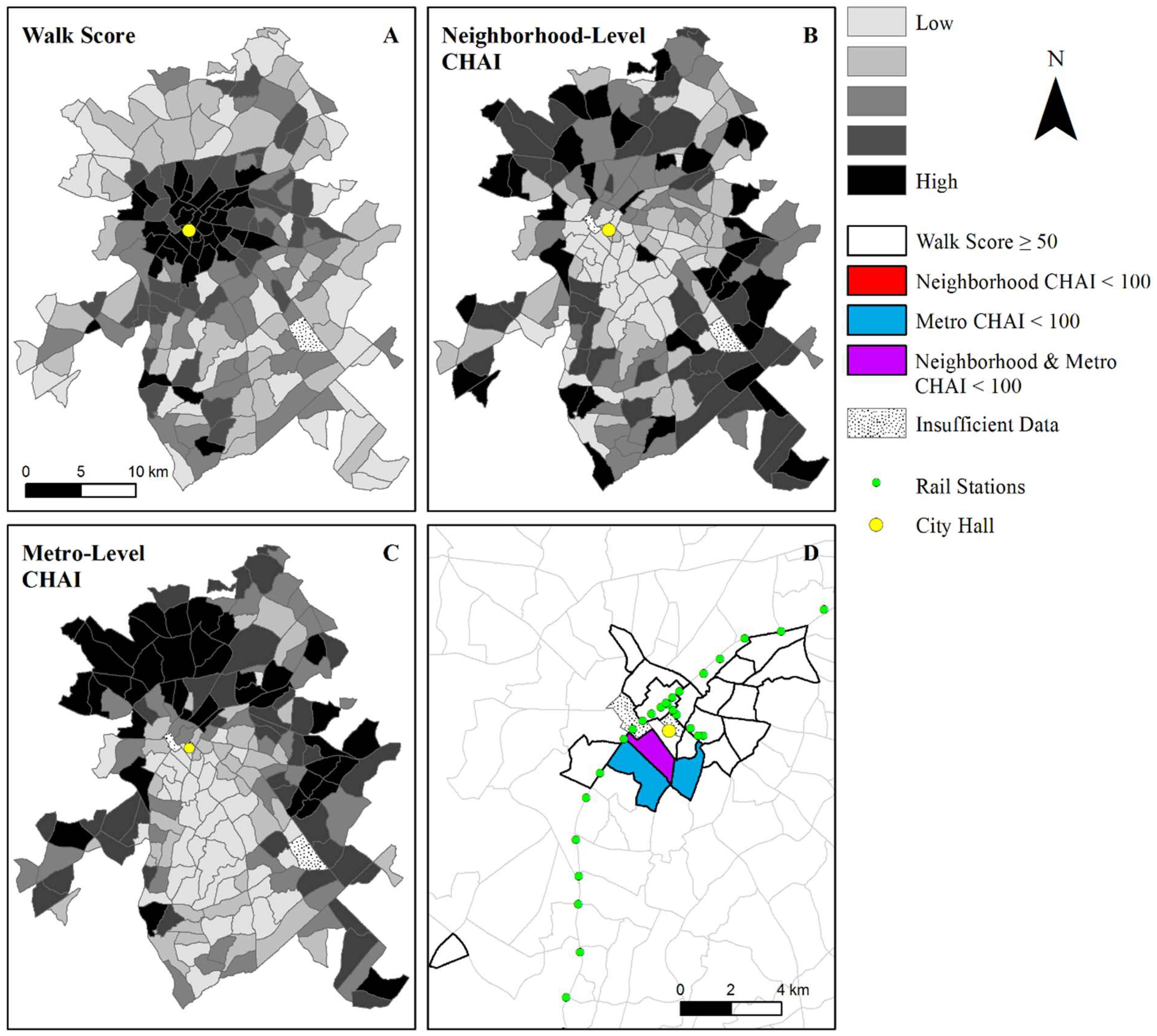
Across the three case study cities (Table 2, Table 3 and Table 4), walk score was a significant predictor of housing affordability in only two models: in Pittsburg at the neighborhood scale and in Portland at the metropolitan scale (renters only). Interestingly, walk score was not a significant predictor of housing affordability for either home owners or renters separately in Pittsburgh, but was significant when considering both owners and renters together using the combined housing affordability index (Table 3). As observed at the national level, housing affordability was negatively associated with walk score at the neighborhood level in Pittsburgh, and the metropolitan level in Portland. That is, median earning households of more walkable neighborhoods in Pittsburgh may experience a modest price premium when controlling for home size and age, while renter households in Portland “saw” more walkable neighborhoods within the metro as less affordable when controlling for crime and housing age. In both Charlotte and Pittsburgh, employment access was significantly and negatively associated with housing affordability, for owners in particular. Similar to the national scale analysis, employment access appeared to overshadow any impact walk score might have on housing affordability for homeowners. This may be especially true for Charlotte, which had few highly walkable neighborhoods, all clustered around the central business district (Figure 1).
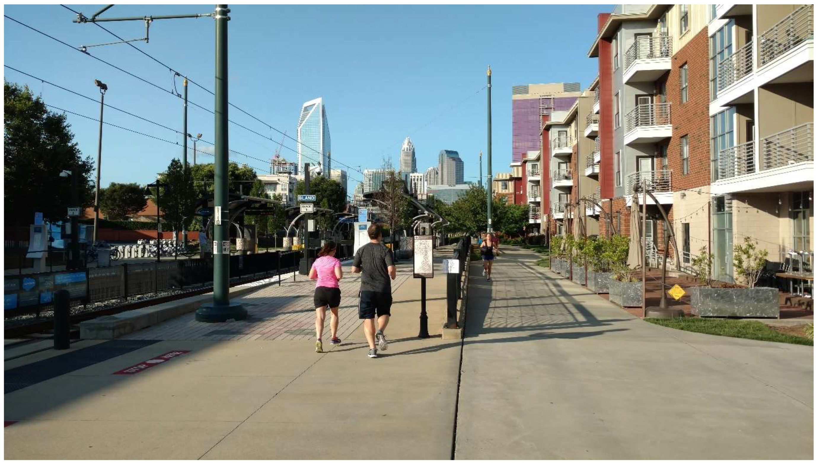
Focusing on each of the three case study areas individually, Figure 1, Figure 2 and Figure 3 highlight distinct patterns of walkability and combined owner/renter housing affordability (CHAI) by census tract. Census tracts with high walkability but low affordability are of particular concern because these represent neighborhoods where walkability, viewed as a positive amenity, may be difficult to afford for the average neighborhood or metropolitan household. In Charlotte, there were relatively few census tracts, mainly clustered around the urban core, with walk scores ≥ 50. Only three of these tracts exhibited relatively low housing affordability (and the potential for housing stress; CHAI < 100), yet this accounted for about 15 percent of Charlotte’s more walkable tracts. Additionally, all three tracts are considered less affordable at the metropolitan scale, suggesting that these neighborhoods (centered around Dilworth and the South End; Figure 4) are potentially unaffordable for median income households residing within the region (and almost certainly unaffordable for lower income, renter households). This area of the city offers enhanced access to the downtown central business district (CBD) and other employment/retail centers along Charlotte’s LYNX light rail system, potentially off-setting some of the housing premium with reduced transportation costs. Note that Charlotte has a relatively affordable housing market overall; the three less-affordable tracts are all located within the more walkable and accessible urban core.
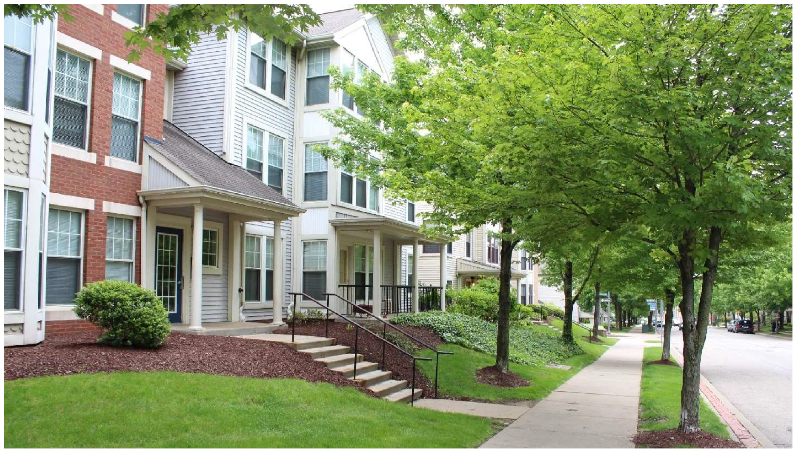
Similar to Charlotte, Pittsburgh exhibited relatively high housing affordability overall, with only six census tracts with CHAI values less than 100 (Figure 2). These “less-affordable” census tracts were also all centrally located, with four of the six having a walk score greater than 50. Nearest downtown, this included two census tracts with low housing affordability for both neighborhood and metro residents. Located within the Hill District of central Pittsburgh, these tracts are home to new infill/redevelopment projects including the Skyline Terrace mixed-income row house development (Figure 5), recently completed in 2016, and the Bedford Hill Apartment townhomes. Importantly, over 90 percent of households within these two tracts are renters, and the annual income disparity between renter and owner households in Pittsburgh is substantial ($30k vs. $67k). Thus, while these areas remain an affordable option for the average owner household, they may represent sites of housing stress for the average Pittsburgh renter household, especially those lacking housing subsidies.
Among the three case study cities, Portland, Oregon exhibited by far the largest number and proportion of “walkable” census tracts, as well as the greatest potential for housing stress among the three case study cities (Figure 3). About half of Portland’s census tracts with less affordable housing—those with a neighborhood or metropolitan CHAI < 100—exhibited walk scores of 50 or above, and 45 percent had walk scores of ≥ 70, indicating “very walkable” conditions. The enhanced walkability and reduced housing affordability may be due in part to Portland’s urban containment policies, most notably the use of an urban growth boundary (UGB), as well as local gains in employment and income [59,60]. The majority of more walkable census tracts with relatively low housing affordability were located within 5 km of downtown (Figure 3E) and included the CBD as well as parts of the popular Northwest District (Figure 6), Irvington/Alameda, and East Portland neighborhoods. Portland also has several auto-dependent neighborhoods with low housing affordability relative to the average Portland household, mainly spread across the forested hills west and south of downtown. Lastly, there appeared to be some housing stress for residents of Portland’s mostly auto-dependent northwestern suburbs, where incomes are moderate but housing costs are relatively high, particularly for home owners. As these three case studies demonstrate, the degree of overlap between high walkability and low affordability census tracts, and their spatial patterns, varied among urban areas, but tended to cluster around the urban core.
4. Discussion and Conclusions
With the exception of the Portland case study, no statistically significant relationship was observed between housing affordability and walkability at the metropolitan scale, suggesting that median income households in many areas of the country currently have adequate access to affordable housing in walkable neighborhoods located within their own metropolitan area. While this may sound encouraging, it is important to emphasize that half of households earn less than the median income, and thus for a significant portion of the population, walkable areas, many of which carry a cost premium [28,30,31,61,62], may be increasingly difficult to afford. It is recommended that future investigations consider housing affordability for households earning perhaps 50 or 30 percent of the median.
For renters and households earning less than the median income already living in walkable neighborhoods, housing stress may be acute; walkability was negatively related to housing affordability at the neighborhood scale across the national sample of census tracts, as well as in Pittsburgh. In Portland, where a statistically significant relationship was observed between housing affordability and walkability at the metropolitan scale, several walkable, inner-city census tracts exhibited relatively low housing affordability for either those living in the neighborhood or for the average metropolitan household. Additionally, all census tracts in Charlotte with particularly low housing affordability were located in a walkable region of the city in close proximity to downtown and the LYNX light rail line. Together, these case studies imply the potential for inequitable access to affordable housing within more centralized, walkable urban communities, echoing concerns raised in previous research [24,25,26,27,63]. Even in those models in which walkability was not a significant predictor of housing affordability, employment accessibility frequently was, with more central and accessible locations most often associated with higher housing stress.
Though new insights have been gained regarding the potential relationships between housing affordability and neighborhood walkability among U.S. urban areas, the present study has important limitations that could be addressed by future research. First, this investigation focused on housing affordability specifically and did not consider additional location-specific household costs such as transportation. Thus, while households may spend more on housing in denser, more walkable neighborhoods, this extra expense could be partially offset with reductions in costs related to automobile ownership and use [34,64]. Transportation costs, however, are highly variable and may be challenging to estimate accurately for the purpose of policy prescription given differences related to household size, geographic location, transportation choices and accessibility, individual preferences and behaviors, among other factors [56]. Nevertheless, the use of a comprehensive location affordability index could provide a more complete view of walkability’s impact on affordability.
Second, the scope of the study could be widened by examining the affordability–walkability nexus in cities higher and lower in the urban hierarchy, as well as cities in other countries. Cities with particularly acute housing shortages, such as San Francisco, San Jose, and New York City, may provide instructive case studies. It may also be fruitful to compare differences in the spatial relationships between affordability and walkability in larger versus smaller metropolitan areas (the three case study metros presented here were of approximately the same size class). Finally, changes in affordability in relation to neighborhood walkability over time would provide a clearer picture of walkability as an equity concern, with forces, such as financialization, neoliberalization, globalization, and gentrification, seemingly placing ever-greater pressure on urban housing markets [65,66,67].
Third, the relationship between housing affordability and walkability is likely to change over time, with gentrification of inner-city neighborhoods being an on-going, dynamic process. To fully gauge whether lower income groups are becoming increasingly excluded from more central and walkable neighborhoods, a time series will be needed to compare changes in affordability with changes in walkability, employment accessibility, and other place-based amenities. Future research should thus attempt to assess and track these variables over time.
Fourth and finally, geographically-weighted regression (GWR) was not utilized in this study due to the non-contiguous nature of the census tracts at the national level, and the relatively limited number (≈200) of census tracts available for each of the three individual case study cities, particularly Charlotte. It may be possible, however, to use GWR to compare more extensive metropolitan areas or to investigate smaller metropolitan areas in which data has been aggregated at a finer areal unit size such as census block groups. GWR may enable a more precise analysis by taking into account local variations in the relationship between dependent (housing affordability) and independent (walkability, etc.) variables [68].
While the results of this investigation demonstrate place-specific variations in the walkability-housing affordability interface, overall there is reason for concern that households earning the median income or below may have more limited access to safe, walkable neighborhoods proximal to job centers. Currently, there appears to be a stronger connection between employment accessibility and housing affordability than between walkability and affordability, suggesting that a more pressing concern may be inadequate affordable housing in employment-rich locations. Policy focused on providing affordable housing in walkable areas with ample transit and employment accessibility should be a priority for city leaders and administrators. The availability of efficient, safe transit systems can reduce household transportation costs and further reduce the financial burden of housing in central, amenity-rich areas with higher land values. As frequently the most visible and significant household expenditure, improving the actual and perceived affordability of housing in walkable urban neighborhoods is paramount to the development of cities that are equitable, sustainable, and inclusive.
Funding
This research received no external funding.
Acknowledgments
The author would like to thank Paul Hunt at the University of Nebraska at Omaha for assisting with data procurement and processing.
Conflicts of Interest
The author declares no conflict of interest.
References
- Sohmer, R.R.; Lang, R.E. Downtown Rebound (FMF Census Note 03); Fannie Mae: Washington, DC, USA, 2001. [Google Scholar]
- Birch, E.L. Having a longer view on downtown living. J. Am. Plan. Assoc. 2002, 68, 5–21. [Google Scholar] [CrossRef]
- Goetz, E.G. Clearing the Way: Deconcentrating the Poor in Urban America; The Urban Institute Press: Washington, DC, USA, 2003. [Google Scholar]
- Zukin, S.; Trujillo, V.; Frase, P.; Jackson, D.; Recuber, T.; Walker, A. New retail capital and neighborhood change: Boutiques and gentrification in New York City. City Community 2009, 8, 47–64. [Google Scholar] [CrossRef]
- Ehrenhalt, A. The Great Inversion and the Future of the American City; Random House, Inc.: New York, NY, USA, 2012; ISBN 978-0307474377. [Google Scholar]
- Florida, R. The Rise of the Creative Class; Basic Books: New York, NY, USA, 2002; ISBN 9780465024766. [Google Scholar]
- Brown, J.; Meczynski, M. “Complexcities”: Locational choices of creative knowledge workers. Built Environ. 2009, 35, 238–252. [Google Scholar] [CrossRef]
- Bereitschaft, B. Neighborhood change among creative-cultural districts in mid-sized US metropolitan areas, 2000–2010. Reg. Stud. Reg. Sci. 2014, 1, 158–183. [Google Scholar] [CrossRef]
- Moos, M. From gentrification to youthification? The increasing importance of young age in delineating high-density living. Urban Stud. 2016, 53, 2903–2920. [Google Scholar] [CrossRef]
- Talen, E. Pedestrian access as a measure of urban quality. Plan. Pract. Res. 2002, 17, 257–278. [Google Scholar] [CrossRef]
- Jabareen, Y.R. Sustainable urban forms: Their typologies, models, and concepts. J. Plan. Educ. Res. 2006, 26, 38–52. [Google Scholar] [CrossRef]
- Tran, M.C. Healthy cities—Walkability as a component of health-promoting urban planning and design. J. Sustain. Urban. Plan. Prog. 2016, 1, 11–21. [Google Scholar] [CrossRef]
- Frank, L.D.; Engelke, P. Impacts of the built environment on health: Walkable places and the exposure to air pollution. Int. Reg. Sci. Rev. 2005, 28, 193–216. [Google Scholar] [CrossRef]
- Lovasi, G.S.; Neckeman, K.M.; Quinn, J.W.; Weiss, C.C.; Rundle, A. Effect of individual or neighborhood disadvantage on the association between neighborhood walkability and body mass index. Am. J. Public Health 2009, 99, 279–284. [Google Scholar] [CrossRef]
- Sallis, J.F.; Saelens, B.; Frank, L.; Conway, T.L.; Slymen, D.J.; Cain, K.L.; Chapman, J.E.; Kerr, J. Neighborhood built environment and income: Examining multiple health outcomes. Soc. Sci. Med. 2009, 68, 1285–1293. [Google Scholar] [CrossRef] [PubMed] [Green Version]
- Leyden, K.M. Social capital and the built environment: The importance of walkable neighborhoods. Am. J. Public Health 2003, 93, 1546–1551. [Google Scholar] [CrossRef] [PubMed]
- French, S.; Wood, L.; Foster, S.A.; Giles-Corti, B.; Frank, L.; Learnihan, V. Sense of community and its association with the neighborhood built environment. Environ. Behav. 2013, 46, 677–697. [Google Scholar] [CrossRef]
- Kamruzzaman, M.; Wood, L.; Hine, J.; Currie, G.; Giles-Corti, B.; Turrell, G. Patterns of social capital associated with transit oriented development. J. Transp. Geogr. 2014, 35, 144–155. [Google Scholar] [CrossRef] [Green Version]
- Frank, L.D.; Sallis, J.F.; Conway, T.L.; Chapman, J.E.; Saelens, B.E.; Bachman, W. Many pathways from land use to health. J. Am. Plan. Assoc. 2006, 72, 75–87. [Google Scholar] [CrossRef]
- Stone, B.; Mednick, A.C.; Holloway, T.; Spak, S.N. Is compact growth good for air quality? J. Am. Plan. Assoc. 2007, 73, 404–420. [Google Scholar] [CrossRef]
- Brueckner, J.K.; Rosenthal, S.S. Gentrification and neighborhood housing cycles: Will America’s future downtowns be rich? Rev. Econ. Stat. 2009, 91, 725–743. [Google Scholar] [CrossRef]
- Goetz, E. Gentrification in black and white: The racial impact of public housing demolition in American cities. Urban Stud. 2010, 48, 1581–1604. [Google Scholar] [CrossRef]
- Myers, D. Peak Millennials: Three reinforcing cycles that amplify the rise and fall of urban concentration by millennials. Hous. Policy Debate 2016, 26, 928–947. [Google Scholar] [CrossRef]
- Neckerman, K.M.; Lovasi, G.S.; Davies, S.; Purciel, J.Q.; Feder, E.; Raghunath, N.; Wasserman, B.; Rundle, A. Disparities in urban neighborhood conditions: Evidence from GIS measures and field observation in New York City. J. Public Health Policy 2009, 30, S264–S285. [Google Scholar] [CrossRef]
- Koschinsky, J.; Talen, E. Affordable housing and walkable neighborhoods: A national urban analysis. Cityscape J. Policy Dev. Res. 2015, 17, 13–56. [Google Scholar]
- Riggs, W. Inclusively walkable: Exploring the equity of walkable housing in the San Francisco Bay Area. Local Environ. 2016, 21, 527–554. [Google Scholar] [CrossRef]
- Bereitschaft, B. Equity in neighbourhood walkability? A comparative analysis of three large U.S. cities. Local Environ. 2017, 22, 859–879. [Google Scholar] [CrossRef]
- Cortright, J. Walking the Walk: How Walkability Raises Home Values in U.S. Cities. CEOs for Cities, August 2009. Available online: http://blog.walkscore.com/wp-content/uploads/2009/08/WalkingTheWalk_CEOsforCities.pdf (accessed on 2 August 2018).
- Rauterkus, S.Y.; Miller, N.G. Residential land values and walkability. J. Sustain. Real Estate 2011, 3, 23–43. [Google Scholar] [CrossRef]
- Sohn, D.W.; Moudon, A.V.; Lee, J. The economic value of walkable neighborhoods. Urban Des. Int. 2012, 17, 115–128. [Google Scholar] [CrossRef]
- Bartholomew, K.; Ewing, R. Hedonic price effects of pedestrian- and transit-oriented development. J. Plan. Lit. 2011, 26, 18–34. [Google Scholar] [CrossRef]
- Olaru, D.; Smith, B.; Taplin, J.H.E. Residential location and transit-oriented development in a new rail corridor. Transp. Res. Part A 2011, 45, 219–237. [Google Scholar] [CrossRef]
- Hass, P.M.; Makarewicz, C.; Benedict, A.; Sanchez, T.W.; Dawkins, C.J. Housing & Transportation Cost Trade-Offs and Burdens of Working Households in 28 Metros; Center for Neighborhood Technology and Virginia Tech: Chicago, IL, USA; Blacksburg, VA, USA, 2006. [Google Scholar]
- Mattingly, K.; Morrissey, J. Housing and transport expenditure: Socio-spatial indicators of affordability in Auckland. Cities 2014, 38, 69–83. [Google Scholar] [CrossRef]
- Mulliner, E.; Smallbone, K.; Maliene, V. An assessment of sustainable housing affordability using a multiple criteria decision making method. Omega 2013, 41, 270–279. [Google Scholar] [CrossRef] [Green Version]
- U.S. Bureau of Labor Statistics. Economic News Release: Consumer Expenditures—2016. 2017. Available online: https://www.bls.gov/news.release/cesan.nr0.htm (accessed on 23 April 2018).
- Kiersz, A. The Economies of the 40 Biggest US Cities, Ranked from Worst to Best. Business Insider. 20 June 2018. Available online: https://www.businessinsider.com/us-economy-by-metro-area-ranked-san-francisco-seattle-austin-2018-4 (accessed on 3 December 2018).
- National Association of Realtors (NAR). Housing Affordability Index: Methodology. Available online: https://www.nar.realtor/research-and-statistics/housing-statistics/housing-affordability-index/methodology (accessed on 10 July 2018).
- U.S. Census Bureau. 2012–2016 American Community Survey 5-Year Estimates. Available online: http://factfinder2.census.gov (accessed on 12 July 2018).
- Piazzesi, M.; Schneider, M.; Tuzel, S. Housing, Consumption and Asset Pricing. J. Financ. Econ. 2007, 83, 531–569. [Google Scholar] [CrossRef]
- Walk Score®. 2018. Available online: https://www.walkscore.com/methodology.shtml (accessed on 24 June 2018).
- Duncan, D.T.; Meline, J.; Kestens, Y.; Day, K.; Elbel, B.; Trasande, L.; Chaix, B. Walk Score, transportation mode choice, and walking among French adults: A GPS, accelerometer, and mobility survey study. Int. J. Res. Public Health 2016, 13, 611. [Google Scholar] [CrossRef]
- Towne, S.D., Jr.; Won, J.; Lee, S.; Ory, M.G.; Forjuoh, S.N.; Wang, S.; Lee, C. Using Walk ScoreTM and neighborhood perceptions to assess walking among middle-aged and older adults. J. Community Health 2016, 41, 977–988. [Google Scholar] [CrossRef]
- McDonald, N.C. The effect of objectively measured crime on walking in minority adults. American J. Health Prom. 2008, 22, 433–436. [Google Scholar] [CrossRef] [PubMed]
- Satariano, W.A.; Ivey, S.L.; Kurtovich, E.; Kealey, M.; Hubbard, A.E.; Bayles, C.M.; Bryant, L.L.; Hunter, R.H.; Prohaska, T.R. Lower-body function, neighborhoods, and walking in an older population. Am. J. Prev. Med. 2010, 38, 419–428. [Google Scholar] [CrossRef] [PubMed]
- Lachapelle, U.; Noland, R.B. Inconsistencies in associations between crime and walking: A reflection of poverty and density. Int. J. Sustain. Transp. 2015, 9, 103–115. [Google Scholar] [CrossRef]
- Hess, D.B.; Almeida, T.M. Impact of proximity to light rail rapid transit on station-area property values in Buffalo, New York. Urban Stud. 2007, 44, 1041–1068. [Google Scholar] [CrossRef]
- Immergluck, D. Large redevelopment initiatives, housing values and gentrification: The case of the Atlanta Beltline. Urban Stud. 2009, 46, 1723–1745. [Google Scholar] [CrossRef]
- Ben-Akiva, M.; Morikawa, T. Comparing ridership attraction of rail and bus. Transp. Policy 2002, 9, 107–116. [Google Scholar] [CrossRef]
- Currie, G. The demand performance of bus rapid transit. J. Public Trans. 2005, 8, 41–55. [Google Scholar] [CrossRef]
- Noland, R.B.; Weiner, M.D.; DiPetrillo, S.; Kay, A.I. Attitudes toward transit-oriented development: Resident experiences and professional perspectives. J. Transp. Geogr. 2017, 60, 130–140. [Google Scholar] [CrossRef]
- Rubin, G.M. Is housing age a commodity? Hedonic price estimates of unit age. J. Hous. Res. 1993, 4, 165–184. [Google Scholar]
- Zhao, N. Half of US Homes Built before 1980. National Association of Homebuilders. Available online: http://eyeonhousing.org/2018/08/half-of-us-homes-built-before-1980 (accessed on 8 August 2018).
- Franklin, J.P.; Waddell, P. A hedonic regression of home prices in King County, Washington, using activity-specific accessibility measures (pp. 16). Presented at the TRB 2003 Annual Meeting, Washington, DC, USA, 12–16 January 2003. [Google Scholar]
- U.S. Department of Housing and Urban Development (HUD). Location Affordability Index Data and Methodology—Version 2.1. September 2016. Available online: https://www.hudexchange.info/resources/documents/Location-Affordability-Index-Data-and-Methodology-V2.1.pdf (accessed on 15 August 2018).
- Glaeser, E.L.; Gyourko, J. The impact of building restrictions on housing affordability. Econ. Policy Rev. 2003, 9, 21–39. [Google Scholar]
- Saiz, A. The geographic determinants of housing supply. Quart. J. Econ. 2010, 125, 1253–1296. [Google Scholar] [CrossRef]
- Hilber, C.A.L. Neighborhood externality risk and the homeownership status of properties. J. Urban Econ. 2005, 57, 213–241. [Google Scholar] [CrossRef]
- Phillips, J.; Goodstein, E. Growth management and housing prices: The case of Portland. Contemp. Econ. Policy 2000, 18, 334–344. [Google Scholar] [CrossRef]
- Cox, W. A Question of Values: Middle-Income Housing Affordability and Urban Containment Policy. Frontier Centre for Public Policy No. 180. , October 2015. Available online: https://fcpp.org/wp-content/uploads/PS180-Cox-A-Question-of-Values_CF1.pdf (accessed on 30 August 2018).
- Li, W.; Joh, K.; Lee, C.; Kim, H.-W.; Park, H.; Woo, A. Assessing benefits of neighborhood walkability to single-family property values: A spatial hedonic study in Austin, Texas. J. Plan. Res. 2015, 35, 471–488. [Google Scholar] [CrossRef]
- Gilderbloom, J.I.; Riggs, W.W.; Meares, W.L. Does walkability matter? An examination of walkability’s impact on housing values, foreclosures and crime. Cities 2015, 42, 13–24. [Google Scholar] [CrossRef]
- Bereitschaft, B. Equity in microscale urban design and walkability: A photographic survey of six Pittsburgh streetscapes. Sustainability 2017, 9, 1233. [Google Scholar] [CrossRef]
- Saberi, M.; Wu, H.; Amoh-Gyimah, R.; Smith, J.; Arunachalam, D. Measuring housing and transportation affordability: A case study of Melbourne, Australia. J. Transp. Geogr. 2017, 65, 134–146. [Google Scholar] [CrossRef]
- Fields, D. Contesting the financialization of urban space: Community organizations and the struggle to preserve affordable rental housing in New York City. J. Urban Affairs 2015, 37, 144–165. [Google Scholar] [CrossRef]
- Marom, N.; Carmon, N. Affordable housing plans in London and New York: Between marketplace and social mix. Hous. Stud. 2015, 30. [Google Scholar] [CrossRef]
- Rosen, G.; Walks, A. Castles in Toronto’s sky: Condo-ism as urban transformation. J. Urban Affairs 2015, 37, 289–310. [Google Scholar] [CrossRef]
- Fotheringham, A.S.; Brunsdon, C.; Charlton, M. Geographical Weighted Regression: The Analysis of Spatially Varying Relationships; John Wiley & Sons Ltd.: Chichester, UK, 2002. [Google Scholar]
Figure 1.
The spatial relationship between (A) walkability and housing affordability calculated at the (B) neighborhood and (C) metropolitan scale for census tracts within the urbanized area of Charlotte, NC. Of particular interest is where (D) relatively high walkability and low housing affordability overlap. The comprehensive housing affordability index (CHAI) was calculated by summing the standardized housing affordability for home owners and renters, and weighing each based on their proportion within each census tract.

Figure 2.
The spatial relationship between (A) walkability and housing affordability calculated at the (B) neighborhood and (C) metropolitan scale for census tracts within the urbanized area of Pittsburgh, PA. Of particular interest is where (D) relatively high walkability and low housing affordability overlap. The comprehensive housing affordability index (CHAI) was calculated by summing the standardized housing affordability for home owners and renters, and weighing each based on their proportion within each census tract.

Figure 3.
The spatial relationship between (A) walkability and housing affordability calculated at the (B) neighborhood and (C) metropolitan scale for census tracts within the urbanized area of Portland, OR. Of particular interest is where (D) relatively high walkability and low housing affordability overlap, most notably prominently around (E) the city center. The comprehensive housing affordability index (CHAI) was calculated by summing the standardized housing affordability for home owners and renters, and weighing each based on their proportion within each census tract.

Figure 4.
Pedestrian corridor and new up-scale housing along the LYNX light rail line southwest of downtown Charlotte, NC. Photo by author.
Figure 4.
Pedestrian corridor and new up-scale housing along the LYNX light rail line southwest of downtown Charlotte, NC. Photo by author.

Figure 5.
Mixed-income development just outside downtown Pittsburgh, PA. Photo by author.

Figure 6.
A walkable streetscape in the fashionable Northwest District, Portland, OR, USA. Photo by author.
Figure 6.
A walkable streetscape in the fashionable Northwest District, Portland, OR, USA. Photo by author.


Table 1.
Results of the OLS regression analysis (stepwise procedure) of randomly selected census tracts (N = 2300) within U.S. urbanized areas, with the log (10) of the combined renter and owner (CHAI), owner only (HAI), and renter only (RAI) housing affordability indices as the dependent variables.
| Neighborhood Scale | Metropolitan Scale | |||||
|---|---|---|---|---|---|---|
| B | S.E. | Sig. | B | S.E. | Sig. | |
| Renter + Owner | ||||||
| Constant | 2.040 | 0.018 | <0.001 | 2.880 | 0.043 | <0.001 |
| Walk Score | −0.002 | <0.001 | <0.001 | -- | -- | -- |
| ‡ Crime Index | -- | -- | -- | 0.040 | 0.005 | <0.001 |
| Rail Within 2 km | -- | -- | -- | -- | -- | -- |
| Coast Within 100 km | −0.088 | 0.006 | <0.001 | −0.085 | 0.007 | <0.001 |
| ‡ Employment Access | -- | -- | -- | −0.069 | 0.004 | <0.001 |
| ‡ % Housing Post-1980 | -- | -- | -- | −0.036 | 0.004 | <0.001 |
| No. Bedrooms | 0.044 | 0.003 | <0.001 | -- | -- | -- |
| Model r2 | 0.398 | 0.267 | ||||
| Owner Only | ||||||
| Constant | 3.018 | 0.051 | <0.001 | 2.89 | 0.087 | <0.001 |
| Walk Score | -- | -- | -- | -- | -- | -- |
| ‡ Crime Index | -- | -- | -- | 0.125 | 0.007 | <0.001 |
| Rail Within 2 km | -- | -- | -- | -- | -- | -- |
| Coast Within 100 km | −0.159 | 0.008 | <0.001 | −0.125 | 0.010 | <0.001 |
| ‡ Employment Access | −0.094 | 0.004 | <0.001 | −0.093 | 0.005 | <0.001 |
| ‡ % Housing Post-1980 | -- | -- | -- | −0.038 | 0.005 | <0.001 |
| No. Bedrooms | 0.042 | 0.003 | <0.001 | -- | -- | -- |
| Model r2 | 0.428 | 0.352 | ||||
| Renter Only | ||||||
| Constant | 2.215 | 0.030 | <0.001 | 1.956 | 0.039 | <0.001 |
| Walk Score | −0.001 | <0.001 | <0.001 | -- | -- | -- |
| ‡ Crime Index | −0.035 | 0.004 | <0.001 | −0.056 | 0.003 | <0.001 |
| Rail Within 2 km | -- | -- | -- | -- | -- | -- |
| Coast Within 100 km | -- | -- | -- | -- | -- | -- |
| ‡ Employment Access | -- | -- | -- | 0.021 | 0.003 | <0.001 |
| ‡ % Housing Post-1980 | -- | -- | -- | -- | -- | -- |
| No. Bedrooms | 0.011 | 0.003 | <0.001 | 0.026 | 0.002 | <0.001 |
| Model r2 | 0.116 | 0.204 | ||||
‡ log-transformed.
Table 2.
Results of the OLS regression analyses (stepwise procedure) for the Charlotte, NC urbanized area, with the log (10) of the combined renter and owner (CHAI), owner only (HAI), and renter only (RAI) housing affordability indices as the dependent variables.
Table 2.
Results of the OLS regression analyses (stepwise procedure) for the Charlotte, NC urbanized area, with the log (10) of the combined renter and owner (CHAI), owner only (HAI), and renter only (RAI) housing affordability indices as the dependent variables.
| Neighborhood Scale | Metropolitan Scale | |||||
|---|---|---|---|---|---|---|
| B | S.E. | Sig. | B | S.E. | Sig. | |
| Renter + Owner | ||||||
| Constant | 2.991 | 0.101 | <0.001 | 3.363 | 0.146 | <0.001 |
| Walk Score | -- | -- | -- | -- | -- | -- |
| ‡ Crime Index | -- | -- | -- | 0.135 | 0.017 | <0.001 |
| ‡ Distance to Rail | -- | -- | -- | -- | -- | -- |
| ‡ Employment Access | −0.075 | 0.010 | <0.001 | −0.175 | 0.018 | <0.001 |
| ‡ % Housing Post-1980 | -- | -- | -- | -- | -- | -- |
| No. Bedrooms | -- | -- | -- | -- | -- | -- |
| Model r2 | 0.230 | 0.345 | ||||
| Owner Only | ||||||
| Constant | 2.143 | 0.058 | <0.001 | 3.456 | 0.233 | <0.001 |
| Walk Score | -- | -- | -- | -- | -- | -- |
| ‡ Crime Index | 0.101 | 0.014 | <0.001 | 0.327 | 0.027 | <0.001 |
| ‡ Distance to Rail | -- | -- | -- | -- | -- | -- |
| ‡ Employment Access | −0.094 | 0.015 | <0.001 | -0.261 | 0.028 | <0.001 |
| ‡ % Housing Post-1980 | -- | -- | -- | -- | -- | -- |
| No. Bedrooms | -- | -- | -- | -- | -- | -- |
| Model r2 | 0.230 | 0.443 | ||||
| Renter Only | ||||||
| Constant | 1.782 | 0.065 | <0.001 | 2.530 | 0.050 | <0.001 |
| Walk Score | -- | -- | -- | -- | -- | -- |
| ‡ Crime Index | 0.045 | 0.013 | <0.001 | −0.111 | 0.010 | <0.001 |
| ‡ Distance to Rail | -- | -- | -- | -- | -- | -- |
| ‡ Employment Access | -- | -- | -- | -- | -- | -- |
| ‡ % Housing Post-1980 | -- | -- | -- | −0.29 | 0.008 | <0.001 |
| No. Bedrooms | -- | -- | -- | -- | -- | -- |
| Model r2 | 0.056 | 0.372 | ||||
‡ log-transformed.
Table 3.
Results of the OLS regression analyses (stepwise procedure) for the Pittsburgh, PA urbanized area, with the log(10) of the combined renter and owner (CHAI), owner only (HAI), and renter only (RAI) housing affordability indices as the dependent variables.
Table 3.
Results of the OLS regression analyses (stepwise procedure) for the Pittsburgh, PA urbanized area, with the log(10) of the combined renter and owner (CHAI), owner only (HAI), and renter only (RAI) housing affordability indices as the dependent variables.
| Neighborhood Scale | Metropolitan Scale | |||||
|---|---|---|---|---|---|---|
| B | S.E. | Sig. | B | S.E. | Sig. | |
| Renter + Owner | ||||||
| Constant | 2.280 | 0.052 | <0.001 | 2.473 | 0.021 | <0.001 |
| Walk Score | −0.001 | <0.001 | <0.001 | -- | -- | -- |
| ‡ Crime Index | -- | -- | -- | -- | -- | -- |
| ‡ Distance to Rail | -- | -- | -- | -- | -- | -- |
| ‡ Employment Access | -- | -- | -- | -- | -- | -- |
| ‡ % Housing Post-1980 | −0.032 | 0.008 | <0.001 | −0.066 | 0.012 | <0.001 |
| No. Bedrooms | 0.033 | 0.007 | <0.001 | -- | -- | -- |
| Model r2 | 0.233 | 0.084 | ||||
| Owner Only | ||||||
| Constant | 2.446 | 0.041 | <0.001 | 1.986 | 0.071 | <0.001 |
| Walk Score | -- | -- | -- | -- | -- | -- |
| ‡ Crime Index | 0.028 | 0.008 | 0.001 | 0.124 | 0.016 | <0.001 |
| ‡ Distance to Rail | -- | -- | -- | -- | -- | -- |
| ‡ Employment Access | -- | -- | -- | -- | -- | -- |
| ‡ % Housing Post-1980 | −0.043 | 0.008 | <0.001 | -- | -- | -- |
| No. Bedrooms | -- | -- | -- | -- | -- | -- |
| Model r2 | 0.140 | 0.155 | ||||
| Renter Only | ||||||
| Constant | 1.816 | <0.001 | <0.001 | 1.074 | 0.170 | <0.001 |
| Walk Score | -- | -- | -- | -- | -- | -- |
| ‡ Crime Index | 0.046 | 0.011 | <0.001 | -- | -- | -- |
| ‡ Distance to Rail | -- | -- | -- | -- | -- | -- |
| ‡ Employment Access | -- | -- | -- | -- | -- | -- |
| ‡ % Housing Post-1980 | -- | -- | -- | -- | -- | -- |
| No. Bedrooms | -- | -- | -- | 0.050 | 0.008 | <0.001 |
| Model r2 | 0.054 | 0.111 | ||||
‡ log-transformed.
Table 4.
Results of the OLS regression analyses (stepwise procedure) for the Portland, OR urbanized area, with the log(10) of the combined renter and owner (CHAI), owner only (HAI), and renter only (RAI) housing affordability indices as the dependent variables.
Table 4.
Results of the OLS regression analyses (stepwise procedure) for the Portland, OR urbanized area, with the log(10) of the combined renter and owner (CHAI), owner only (HAI), and renter only (RAI) housing affordability indices as the dependent variables.
| Neighborhood Scale | Metropolitan Scale | |||||
|---|---|---|---|---|---|---|
| B | S.E. | Sig. | B | S.E. | Sig. | |
| Renter + Owner | ||||||
| Constant | 2.773 | 0.060 | <0.001 | 3.147 | 0.078 | <0.001 |
| Walk Score | -- | -- | -- | -- | -- | -- |
| ‡ Crime Index | -- | -- | -- | -- | -- | -- |
| ‡ Distance to Rail | -- | -- | -- | -- | -- | -- |
| ‡ % Housing Post-1980 | -- | -- | -- | -- | -- | -- |
| ‡ Employment Access | −0.060 | 0.006 | <0.001 | -0.097 | 0.007 | <0.001 |
| No. Bedrooms | -- | -- | -- | -- | -- | -- |
| Model r2 | 0.238 | 0.306 | ||||
| Owner Only | ||||||
| Constant | 2.941 | 0.064 | <0.001 | 3.428 | 0.133 | <0.001 |
| Walk Score | -- | -- | -- | -- | -- | -- |
| ‡ Crime Index | -- | -- | -- | -- | -- | -- |
| ‡ Distance to Rail | -- | -- | -- | -- | -- | -- |
| ‡ % Housing Post-1980 | -- | -- | -- | -- | -- | -- |
| ‡ Employment Access | −0.071 | 0.006 | <0.001 | -0.117 | 0.013 | <0.001 |
| No. Bedrooms | -- | -- | -- | -- | -- | -- |
| Model r2 | 0.279 | 0.197 | ||||
| Renter Only | ||||||
| Constant | 2.146 | 0.026 | <0.001 | 2.382 | 0.031 | <0.001 |
| Walk Score | -- | -- | -- | −0.001 | <0.001 | 0.002 |
| ‡ Crime Index | -- | -- | -- | −0.051 | 0.007 | <0.001 |
| ‡ Distance to Rail | -- | -- | -- | -- | -- | -- |
| ‡ % Housing Post-1980 | -- | -- | -- | −0.028 | 0.005 | <0.001 |
| ‡ Employment Access | -- | -- | -- | -- | -- | -- |
| No. Bedrooms | −0.022 | 0.005 | 0.001 | -- | -- | -- |
| 0.059 | 0.288 | |||||
‡ log-transformed.
© 2019 by the author. Licensee MDPI, Basel, Switzerland. This article is an open access article distributed under the terms and conditions of the Creative Commons Attribution (CC BY) license (http://creativecommons.org/licenses/by/4.0/).
Share and Cite
MDPI and ACS Style
Bereitschaft, B. Neighborhood Walkability and Housing Affordability among U.S. Urban Areas. Urban Sci. 2019, 3, 11. https://0-doi-org.brum.beds.ac.uk/10.3390/urbansci3010011
AMA Style
Bereitschaft B. Neighborhood Walkability and Housing Affordability among U.S. Urban Areas. Urban Science. 2019; 3(1):11. https://0-doi-org.brum.beds.ac.uk/10.3390/urbansci3010011
Chicago/Turabian StyleBereitschaft, Bradley. 2019. "Neighborhood Walkability and Housing Affordability among U.S. Urban Areas" Urban Science 3, no. 1: 11. https://0-doi-org.brum.beds.ac.uk/10.3390/urbansci3010011