Effects of Urban Development Praxis on Economic Inequality in Latin American Cities


1
Department of Urban Planning, Universidad Simón Bolívar, Sartenejas, Miranda 1080, Venezuela
2
Department of Processes and Systems, Universidad Simón Bolívar, Sartenejas, Miranda 1080, Venezuela
*
Author to whom correspondence should be addressed.
Urban Sci. 2019, 3(3), 88; https://0-doi-org.brum.beds.ac.uk/10.3390/urbansci3030088
Submission received: 30 June 2019
/
Revised: 25 July 2019
/
Accepted: 30 July 2019
/
Published: 5 August 2019
Abstract
:In a highly and rapidly urbanized world, the effect of the action of urban development is determinant for the physical, social, and economic conditions of its citizens, among which is inequality. It is even more crucial for developing regions such as Latin America on which this research is conducted. Therefore, the focus of the investigation was to determine the existence of significant statistical relationships between urban development and economic inequality in the region. For this purpose, it was sought to define urban development from the perspective of the praxis of multilateral organizations measured by indicators of extensive use among them. A hierarchical multiple linear regression model was built with six urban development variables predictors of the Gini coefficient as an indicator of economic inequality, in which data of 49 Latin American cities was used. The application of the method allowed us to discover a stochastic behavior of interaction between those multidimensional systems and confirmed the statistical relation. The research allows having a tool for the formulation of public policies that seek to strengthen local governance, promote community organization and participation, and assert urban planning as an agent for concerted efforts to achieve common goals.
1. Introduction
In the Global South, and particularly in Latin America and the Caribbean, international organizations such as the Interamerican Development Bank (IADB), the Development Bank (CAF), and the World Bank have undertaken massive urban development endeavors. Given the mandate of these organizations, development efforts are usually measured in terms of economic progress and infrastructure but the true impact on the conditions of life of citizens is difficult to account for. Nevertheless, there are key differences between theory and practice; therefore, it is important to establish what the multilateral agencies are seeking when they engage themselves in urban projects in the region, for what a comprehensive analysis of the targets and indicators with which they measure the outcome of projects is key.
The first approximation of international efforts to approach development was based on the theory of economic development. In the context of this work, economy refers to the “(…) study of the use that individuals and societies choose to make scarce resources received from nature and from past generations” [1] (p. 2).
The main concern of economic growth is the scarcity of resources in opposition with the incessant growth of needs generating a progressive increase in the value of goods and services produced in a given territory [2]. On the other hand, economic development includes, in addition to increasing income or production, changes in the social and economic structure, particularly those that allowed for job creation, price stability, and equilibrium of the balance of payments that in the end result in the necessary stability for reaching human potential.
This inference revolves around what theorists like Meier [3] call “The Problem of Underdevelopment”, when beginning to study the limitations of certain countries, not coincidentally in Africa, Asia, and Latin America, to achieve living standards for the majority of its population comparable to the industrialized countries, despite increasing their GDP. This gave way to the inclusion of new variables such as institutionality, freedom, and capacity in the pursuit of development.
In this way, there began to emerge in the academy and the newly created organizations for the development such as the Economic Commission for Latin America and the Caribbean (ECLAC) established in 1948, the Organization for Economic Cooperation and Development (OECD) in 1961, and the United Nations Development Program (UNDP) in 1966, different theories that were looking for explanations of this phenomenon and establish a path towards development.
Basically, development is not achieved solely with money, since a country in conditions of unhealthiness, illiteracy, and in which there are sectors of the population living in poverty cannot be considered “developed” even though its GDP increases considerably and steadily, “(…) the realization of human potential requires much more than what can be expressed in purely economic terms” [4] (p. 5). This was further theorized by Amartya Sen, who focused on terms beyond economy in three fundamental concepts: freedoms, capacity, and agency [5], that led to the emergence of a new, broader and exhaustive concept of human development.
This investigation focuses on the city since it was the core of this industrialized, growth-focused development and the showcase of its effects. The great metropolis of the industrialized countries lived, and even today live, dramatically different conditions from those of the so-called underdeveloped countries, especially in the rural areas. While academia and multilateral organizations were still thinking about a solution to the problem of development, in parallel, the least favored inhabitants sought at all costs to enjoy that prosperity. Many thought that the answer was in the city and migrated looking for greater opportunities for progress, giving way to an accelerated urbanization process. Not in vain, ECLAC pointed out in the early 1960s that “the accelerated rate of growth of our urban population has had serious human and social repercussions derived from the need to assimilate and adapt large masses of rural population to the new ways of life that it imposes the city” [6].
Since the beginning of this argument, the worldwide importance of the pursuit of development was established and, particularly, the impact that urban conditions may have on it. However, the amount of academic studies in this area continues to be proportionally low. Even lower is the amount of quantitative research that allows establishing with statistical rigor the incidence of urban actions on inequality, despite there being several that assert their relationship, at least conceptually, like the works of Abrams [7], Harvey & González [8], and Tur [9].
Another element that makes the study relevant is the decision to perform it on the measurement of existing indicators in Latin American cities. This interest is not political or ideological but rather intends to benefit from the comparison possibility of regional studies. This particularity could establish the predictive equation product of this research as a planning and decision-making tool for local actors, particularly in the framework of urban public policies, given that it is not focused on a single case and is replicable in any context with the only condition that the same indicators are handled and the method is followed. However, a more comprehensive set of indicators could allow expanding the model in the future if new data is collected.
Having defined the problem area and stating the premises and hypotheses that lead to its understanding, the following research objective was established: to investigate if in Latin American cities there exist significant statistical relationships between urban development and economic inequality, to identify the effects of urban praxis on the distribution of income in cities.
2. Urban and Economic Dimensions
One of the main tasks for finding relations between urban development and economic inequality was the selection of indicators that could be calculated and compared, with the idea of finding a way to measure urban practice. Since the city is a complex system, its development cannot be measured with a single element. Inequality, on the other hand, has a different problem since several methodologies and indicators exist, but there is a debate on which is most applicable to a city.
2.1. Dimensions of Urban Development
In order to assess urban development, this investigation reviewed the indicators used by the main actors of Latin American projects, namely the IADB, CAF, UNDP, and UN-Habitat. The Emerging Sustainable Cities (ECS) initiative of the IADB [10] and the UN reports on the state of cities [11,12] served as a framework for what is understood by practitioners as a model for cities. Out of these sources, five dimensions were defined to characterize urban development.
2.1.1. Demography and Size of the City
Size is one of the most common elements to categorize cities; most official organs separate urban and rural in terms of it. When analyzing the different datasets, the size of a city is mainly measured by three indicators: the amount of population that lives in it, whether it includes a metropolitan conurbation area or not, and a relation of both elements, known as density, which gives an idea of how the people are organized in the space. All three indicators were preselected as part of the demography dimension.
2.1.2. Housing and Services
The next dimension is housing, understanding that the main reason behind the act of building is to provide shelter but it is not the only concern when developing an urban area. Even the Universal Declaration of Human Rights ensures the right to a dignified living place and the UN Office of the High Commissioner on Human Rights defines the minimum conditions for a living place, which include proprietorship, availability of services, materials, infrastructure, accessibility, location, and cultural adequacy [13].
In order to measure the status of housing, both quantitative and qualitative deficits were included. IADB [14] considers a quantitative housing deficit when more than one household shares the same roof and food preparation facilities, quantifying it throughout the region. When the deficit is qualitative or functional, they are called precarious or informal settlements (in Latin America they are known as barrios, favelas, or slums depending on the country). Officially, they are settlements that lack one or more of the following elements: durable structure that protects against extreme weather conditions, sufficient defined space as at least one room for every three people, easy access to drinking water in sufficient quantities and at affordable prices, access to adequate sanitary infrastructure, and security of tenure that prevents forced evictions [15].
Slums may appear in the peripheries as a result of the forced integration of new migrants into the city or in central areas, products of changes in the intensity of use, or deterioration of historical sectors and vulnerable areas [16]. It is important to include such an indicator because it is estimated that about 30% of the world’s population lives in these types of settlements [11] and because of the fact it is the first way of expansion of the city. Nowadays, slums are a big focus of most Latin American cities urban public policy agenda.
2.1.3. Public and Green Areas
Space not devoted to buildings is the organizing element of the urban tissue. Public space is defined as “places of common use with no restrictions or control elements apart from those of the civic coexistence” [17]. It is a very important element according to the reviewed sets of indicators. Green spaces may or may not be considered part of them, but the used indicators divide both types. This dimension is included in the investigation because they put an order in the city and serve as an opportunity for exchange and engagement of citizens, even providing identity to the cities.
2.1.4. Transportation and Mobility
Transportation, both private and public, is a defining element of the capacity of a city and another organizing element. A well planned, functioning transport system is key for sustainable development. CAF is particularly focused on this in most of their projects, specifically in two areas: transport infrastructure which includes streets, sidewalks, equipment, and the vehicle fleet; and accessibility in terms of location and related activities. Under this concept, transportation comprises motorized mobility, cycling, and walking.
2.1.5. Planning
The last studied dimension was the actual activity of planning. Both local and national governments are expected to organize and coordinate development efforts with the participation of public, private, and community stakeholders. The main product of that process is an Urban Plan, which becomes enforceable with an instrument of binding law, whether it is a construction code or zoning legislation within a municipal ordinance. Nevertheless, the planning process does not stop there, and the application of the plan should be evaluated and updated. Therefore, they are two main elements when analyzing the status of planning of a city: if a plan exists and has been timely adjusted (less than ten years), and if such plan is enforced and fulfilled.
2.2. Indicators of Economic Inequality
Inequality is “a socioeconomic situation in which a community, social group or collective has unfavorable conditions in comparison with the rest of the environment they belong to” [18]. There are several types of inequality, including social, economic, gender-based, or racial; nevertheless, this investigation focuses on economic inequality, particularly under the capabilities approach of Amartya Sen [19].
There is also a huge debate on objective measurements of economic inequality; most indicators choose a compound method of calculation including different statistical measurements. In order to select a sole indicator for this investigation, it had to follow a set of criteria [20] including independence of scale, variation with transfers from rich to poor households, additive decomposition and a proper rank to include it in a regression. An added criterion was that it had to be measured in cities, and not only nationwide. Several indicators were compared, such as the Atkinson Index, Dalton Index, and Theil index; nevertheless, for international organizations, the most widely used indicator serving as a source for urban data is the Gini Coefficient.
Gini Coefficient
This indicator measures the distribution of income in households by comparing an actual, census-measured reality in a Lorenz Curve with a situation of complete equality [21]. The calculation method used was the World Bank’s [22]. In order to complement the understanding of the inequality situation in each city, it was useful to compare it with the national context; for that, measures of Human Development Index [23], Gross Domestic Product, and population under the National Poverty Line as determined by the census were used to assess countrywide conditions and provide another level for the model.
3. Materials and Methods
This study examines the problem area by first studying variables that can characterize urban development in accordance with international organizations indicators and an indicator of economic inequality in Latin American cities that can be comparable. With that, it establishes the following research questions: is there a statistically significant relationship between them? And, if so, what are possible explanations for that relation? Answers for these questions were sought following the critical multiplism methodological approach, which “consider[s] the simultaneous and complementary use of multiple theories” [24] (p. 53). Seeking probabilistic causality, given the complexity and dynamism of the city as an eminently social system, a deterministic approach would be a mistake.
For the design of the investigation, “Cook’s Decalogue” [25] was followed. It suggests the following steps to ensure a critical multiplism approach in social sciences studies: to establish multiple operational definitions, the use of multiple evaluation methods, to establish programs based on multiple interconnected studies, to perform synthesis from multiple independent studies, to build multivariate causal models, to ask questions about value issues, and to use multiple theoretical approaches as well as performing multiple data analyses and establish objectives that allow a heterogeneous analysis of the results. According to Dunn [26], critical multiplism allows more reliable results for the design and evaluation of public policies.
In order to find relations between the chosen variables, the most appropriate method was to build a multiple linear regression (MLR). Economic inequality was set as the dependent variable and the different urban development descriptors as independent variables. For the multiple linear regression results and the resulting relations to be valid, a series of assumptions must be proven [27,28,29,30]; those are:
- The dependent variable is continuous and approximately normal, as proven using the Shapiro–Wilks test given that the sample is under 50 elements [31].
- Relations between independent and dependent variables are linear, as proven by observing the pattern shown by scatter plots.
- Atypical data was checked by measuring the Mahalanobis distance of data points apart at least three times the interquartile range from the mean.
- There is an absence of multicollinearity, as shown by calculating the Pearson correlation coefficient over 0.70 and significance over 0.300 and checking that variance inflation factors are under 3.000 [28].
- Residuals are independent, which is tested with a Durbin–Watson statistic between 1.5 and 2.5 [32].
- Residuals are normal, shown by applying the Shapiro–Wilks test.
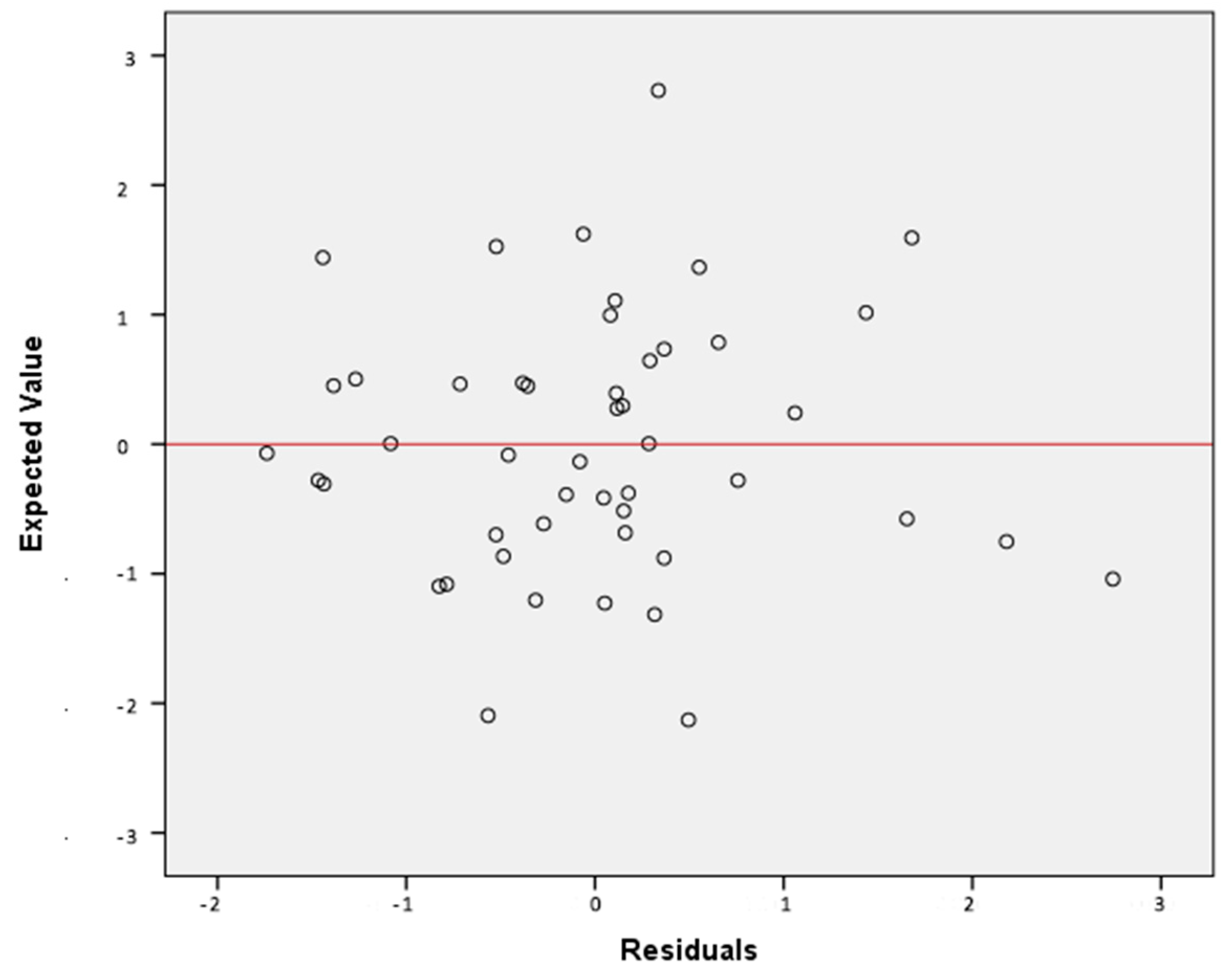
- Residuals are homoscedastic, observing the scatter plot of residues and expected values.
Even when the mathematical and statistical expression of a phenomenon seems clear and straightforward, for empirical cases using real field data, there has to be an iterative operation in order to ensure that the model obtained is adjusted to the initial objectives. Several trial models had to be built with the available variables. With the idea of a more rigorous process, this investigation used the hierarchical regression technique, which is a more complete model that introduces variables to the regression in different hierarchical levels [33]. In this specific case, there were two levels of evaluation: National, for indicators measured in the whole country; and Local, for those measured in cities in which the dependent variable was put. Variables in both levels were grouped in blocks, according to their dimension and whether they are urban or economic. This technique ensures that difference of means and variance does not affect the adjustment of the regression, ending up with a more homogenous result.
The authors carried out the organization of data, calculations, and elaboration of tables and graphics using the software IBM Statistical Package for Social Science SPSS©.
3.1. Design of the Investigation
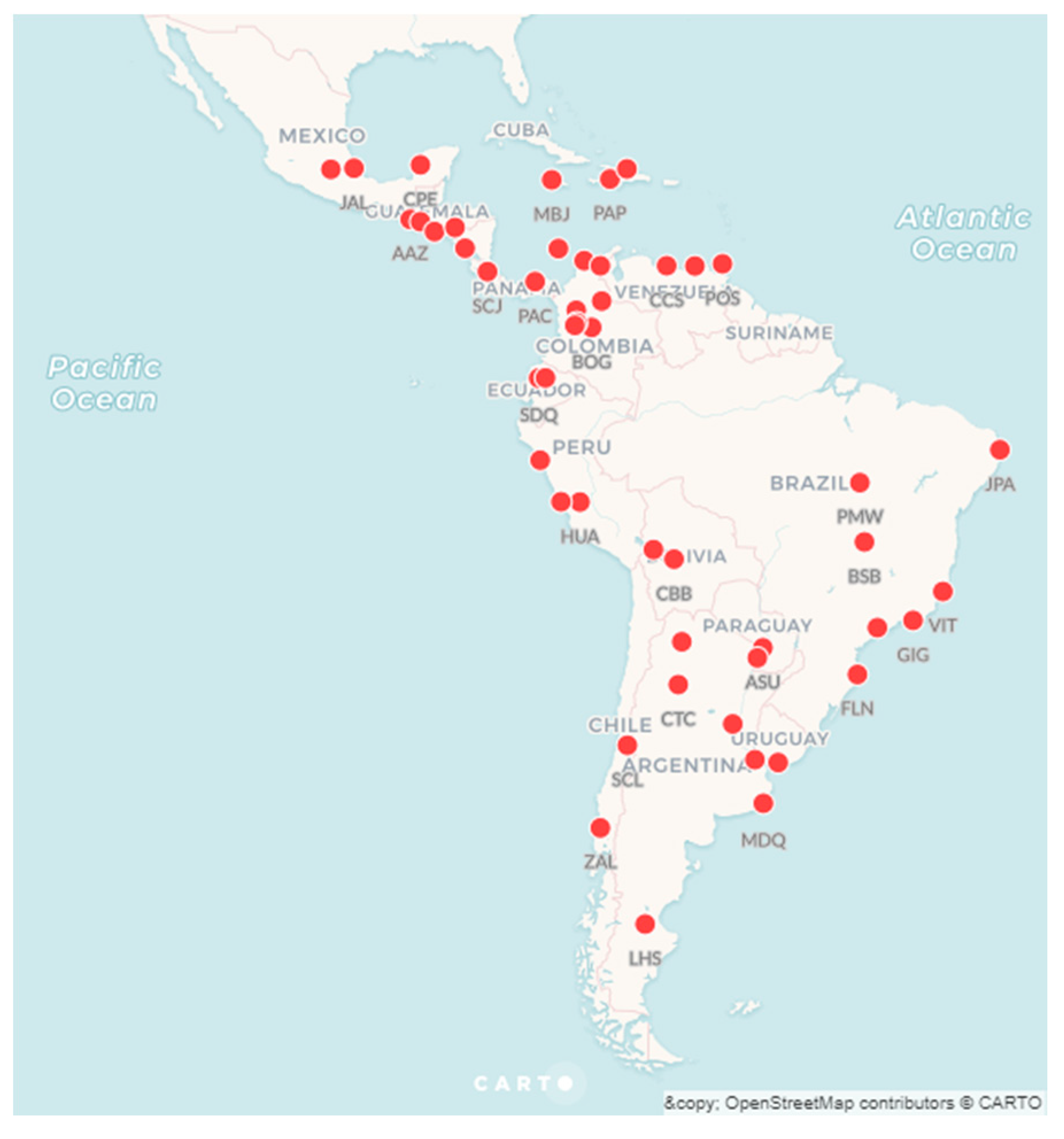
Since this is pre-eminently an urban study, the fundamental unit of analysis was the city. Criteria for the selection of cities was first the definition of Latin America, which for this dataset also includes the Caribbean with a heterogeneous sample of cities in terms of size and growth. The amount of the selected cities depended on data availability and on ensuring statistical significance, given the fact that the final number of elements would define the number of variables that could be included in the regression. Finally, 49 Latin American cities from 21 different countries were selected as shown in Figure 1. A full list of the cities is available in Supplementary Spreadsheet S1.
The variables and their operational definitions follow from the urban dimensions previously identified as well as the selected economic inequality indicator, both of which are detailed in Table 1. To facilitate reporting, from this point onwards the variables will be referred to by code.
3.2. Sources of Data
Data of the 49 cities was obtained for the years 2010 to 2013, the main source was the Urban Dashboard from the IADB which gathers 150 indicators for the participant cities of the ESC initiative [14]. It was complemented by the information available by the World Council on City Data project [34] which is constantly updated by the local governments and the 2014 revision of the UN World Urbanization Prospect [12].
Before adding any data to the investigation, it was checked that calculations of indexes and densities were made using the same formulas, units were converted to follow the SI in case they were not already following it, and USD was always used as currency. Those considerations helped to ensure homogenously-collected data, and therefore, to set up a valid cross-comparison.
3.3. Limitations
Due to the lack of uniform measurements and the outdated statistical information in developing countries, especially at the city scale, most of the indicators had to be taken from the same sources (mainly IADB) which constricted the amount of cities that were able to be included in the research, and in turn, also the amount of variables in the model.
Another main limitation was the fact that despite having some reports and publications from the CAF regarding transport data in Latin America, no comprehensive indicator could be found in a sufficient number of cities to have it included in the regression; therefore, this dimension had to be excluded from the MLR.
3.4. Transformations and Adjustments
Once the data was obtained and organized as it can be seen in Supplementary Spreadsheet S1, the first step of the process was to ensure the fulfilment of the MLR assumptions. Two situations broke the assumptions: nonlinear relations between the variables POB, SUP, VER, and PUB; and a qualitative nominal variable with more than two cases: PLA.
Before considering variables as fit for the MLR, a correlation analysis was carried out to ensure that variables were not redundant and to have an initial understanding of the statistical relationship between each variable and GIN providing insight as to which variables could be eventually introduced in the final model. Using the Pearson Coefficient and the bilateral significance as shown in the Supplementary Table S2, it was determined that there is a significant correlation between variables IDH, PIB, and LPO; between LOGPOB and LOGSUP; and finally, between LOGVER and LOGPUB. Since the correlation appears in variables of the same block, in order to avoid breaking the multicollinearity assumption, only one variable of each block should be introduced in the MLR. The PLA variable could not be analyzed with the same tool because it is a nominal variable; instead, the investigation compared its grouped means for each category with GIN and a one-way ANOVA, as shown in Supplementary Table S2, discovering a significant (p-value < 0.05) relation between both variables.
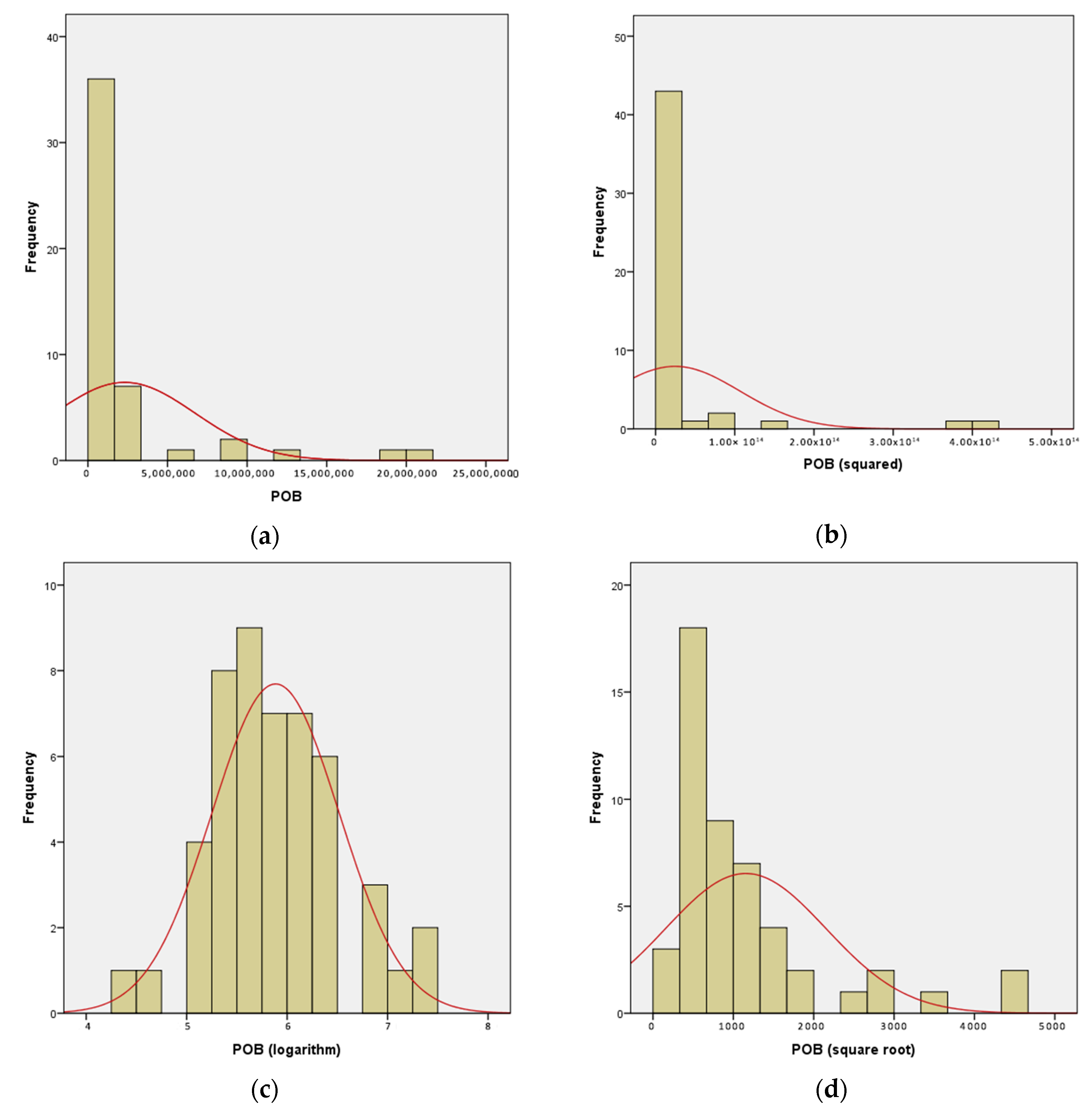
To adjust the nonlinear variables, a transformation had to be made. In order to determine the best one, variables were subject to squaring, logarithm, and square root transformations. Since all presented a similar positive asymmetry and in order to avoid overfitting [35], only one transformation was selected for them. The chosen transformation was logarithmic because it provided the most adjusted curve to the normal distribution and corrected the nonlinearity with the dependent variable as shown in the example of Figure 2. The new, transformed variables are identified as LOGPOB, LOGSUP, LOGVER, and LOGPUB.
The case of the planning variable (PLA) was easily corrected with the creation of two dummy variables (PLA_D1 and PLA_D2) any possible case of the original variable is represented by a combination of the two dummies. Table 2 shows the configuration of the dummies.
4. Results
According to the described method, this investigation analyzed the set of 12 variables that are acceptable in the MLR; nevertheless, it does not mean that all of them can or should be introduced. In this section, that selection was carried out and test models were studied in order to choose the best-fitting model that showed the existence of statistically significant relations between the urban development variables and the economic inequality.
4.1. Selection of Variables
The proper adjustment of the statistical results of an MLR model is defined by its statistical power and significance, which determine the size sample and the maximum number of independent variables that can be introduced. For this investigation, which deals with open systems and social sciences, an acceptable significance of α = 0.10 [30] was defined to ensure at a 90% level of confidence that observations are not due to chance. Since the datasets comprise 49 units of analysis and in order to maintain the statistical power at least at 80% [36], a maximum number of six independent variables may be entered in the model.
Following these considerations, the process of selecting a smaller set of variables out of the initial 12 was executed using the criteria of Prager [37] and ensuring that the selected variables do not belong to the same block. First, a preliminary nonhierarchical model was calculated in SPSS© with all variables to obtain the p-values that are shown in Table 3.
Using these values, three strategies were followed to select the best fitting variables for a model: First, the six variables with a smaller p-value disregarding the blocks. Second the variable with the smaller p-value in each block but both dummies; and third, only variables with a p-value < 0.10. These combinations of variables allowed for three test models to be built and compared.
4.2. Regression Model
The final MLR model of this investigation will be the one that shows a better adjustment under the established parameters of power and significance; to decide this, the test models were compared using the Prediction Criterion (Cp) of Mallow and the Bayesian Information Criterion (BIC) of Schwarz [38]
Test Model 1 was made with the combination of PLA_D1, LOGPUB, PLA_D2, BAR, VIV, and PIB; variables with the lower p-values. A stepwise regression produced the results shown in Table 4.
The second test model included one variable per block; specifically, the one with a lower p-value and both dummy variables to complete the maximum of six, which were: PIB, LOGSUP, BAR, LOGPUB, PLA_D1, and PLA_D2. The regression results are shown in Table 5.
Finally, the third test model included only the variables with p-value < 0.10, even when it does not use the maximum number of variables. The used variables were PLA_D1, LOGPUB, PLA_D2, BAR, and VIV. This model produced the results shown in Table 6.
Comparing each criterion by the Mallows Cp, the three models are fitting, since it equals the number of variables plus a constant. By the Schwarz BIC, the model with the lowest observation is most convenient, in this case, Test Model 2 with −259.685. Finally, as a sign of adjustment, the adjusted R2 was compared, out of which Test Model 2 was again the better suited with 0.503.
Therefore, a two-step MLR Model was calculated to inquire if significant relations exist between economic inequality, characterized by the Gini coefficient (GIN), and the effect of urban development praxis based on variables PIB, for the national context; LOGSUP for size of the city; LOGPUB for public spaces; and PLA_D1 and PLA_D2 to show the planning status. A significant regression equation was found
The predicted Gini coefficient of the city (GIN) is given by
The significance and effect of independent variables on GIN are shown in Table 7.
The remaining assumptions were nonmulticollinearity as well as independence, normality, and homoscedasticity of residuals. For multicollinearity, VIF and tolerance were obtained for each variable; all complied with >3.00 and <0.300, respectively [28], validating the assumption. Then, a Durbin–Watson value of 1.957 confirmed the independence of the residuals. To prove normality, a Shapiro–Wilks test was used and the result of 0.953 with 0.05 significance confirms it. Finally, homoscedasticity was also confirmed by the graphic shown in Figure 3.
With all assumptions proved, the MLR confirms that 49.9% of the variation of the Gini coefficient of these 49 cities can be explained by its urban development conditions, with a significance of p < 0.000 and standard error of 0.05849, well within the confidence interval.
5. Discussion
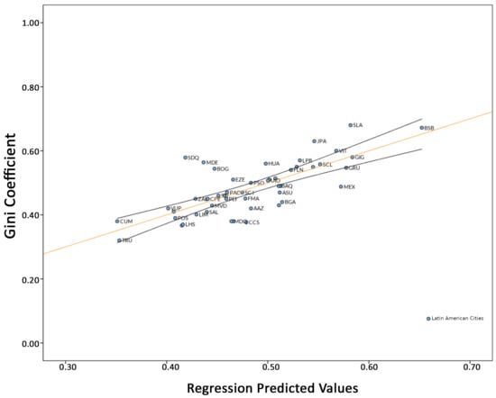
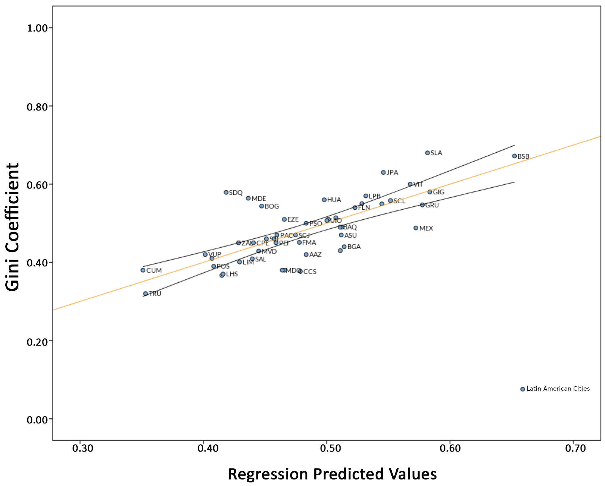
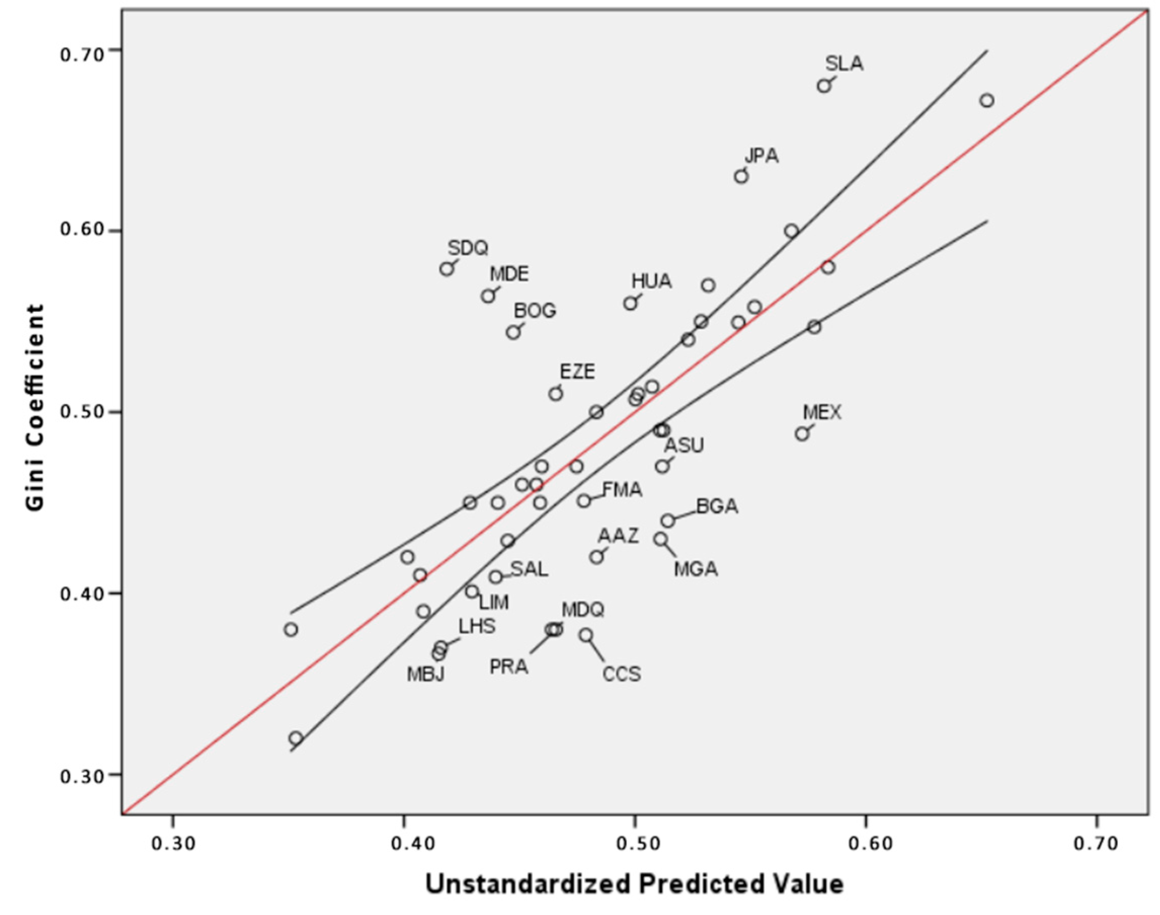
The predictive equation takes Gini values that range from 0.35 in the case of CUM (Cumana, Venezuela) up to 0.65 in the case of BSB (Brasilia, Brazil). It has a mean of 0.48 with a 0.062 standard deviation, this mean value shows a lower inequality than the world average of 0.63 [39] but it is still high according to UN standards, a situation that poses a risk of social unrest. The behavior of the prediction against empirical values may be seen in the scatter plot of Figure 4, which compares both sets with confidence intervals of the size of the mean.
Confirming the coefficient of determination, half of the cities present values well within the interval, if not on the prediction line. Certain cases stand out for having considerable differences with the prediction. In the lower extreme, we find CCS (Caracas, Venezuela) with a Gini measure lower than the one predicted by the equation, which can be explained by the political and economic instability of the country, which has proved to skew inequality measures in transitional countries [40]. In addition to that, Caracas is the objective of central public expense policies which produce an apparently better situation of the capital against the rest of the country [41]. Finally, government-led policies have deliberately tackled the Gini coefficient as an indicator and, in statistical terms, they have achieved their goal; nevertheless, it has not sustainably improved the living conditions of the population [42].
Medellín (MDE) and Bogotá (BOG) can also be explained from the national context. Colombia has been implementing a housing stratification policy since the 1980s to guide public investment, social programs, and even the cost of public services, education, and taxes [43]. Several authors [44,45] argue that this produces stereotypes and segregation, restricting the access of certain sectors to enjoy the benefits of public policy because sometimes the stratification method is not a reliable source to determine payment capacity and subsidy policy. In addition, in the long term, the policy has generated a heterogeneous distribution of the offer of services, equipment, and spaces. The segregation as a producer of inequality is exemplified by the Colombian case.
An ongoing urban process can condition the current situation of inequality, like in the case of Santiago de Chile (SCL). Land policies and their influence on the real estate and housing market of social interest are an element of great importance in urban planning, according to Calavita and Mallach [46]. When allocating land in private hands for projects of social interest, cost is transferred to developers and local authorities generate incentive policies to offset these obligations. The particular case of Santiago “shows us virtues and defects of this joint strategy (…) the housing problem is minimal in terms of quantity (but) the problem has been transferred to the housing and city conditions of the homes produced” [47] (p. 3). In addition to the land dilemma, the predominance of the private over land and housing policy has caused “remote and socially segregated location of social housing remained a characteristic note of housing policy” [48] (p. 12). Again, segregation and marginalization have an important effect on the inequality of a city that, in theory, has good urban conditions in a country with the highest HDI in the region.
The following cases present an inverse situation, the inequality is less than the value predicted by the regression equation. In Argentina, Mar del Plata (MDQ) and Paraná (PRA) are examples of how, in situations of fiscal income, abundant poverty is generalized, a situation that combined with the effects of a sustained economic crisis over time have significantly contracted the revenue of the population, reducing inequality but with an increase in poverty [49]. Mar del Plata also shows an effect of tax corruption. According to a study by the National University of Mar del Plata, two things occur simultaneously. First, citizens with higher incomes tend to declare less income to reduce their taxes and the poorest citizens declare more than they actually receive, as a result of what they call the “shame effect” [50] (p. 8). For this reason, statistics show a much smaller income gap than actually exists.
In the upper extreme, we find that SDQ (Santo Domingo, Dominican Republic) is the city with the most relative error in the prediction. According to Oxfam International [51], this is due to political reasons. Political and economic power are tightly attached and are monopolized in main cities, especially Santo Domingo. The Dominican government alleges that the high inequality is produced by the adverse effect of continued recession cycles that the island has suffered and had, in turn, deteriorated the purchasing power of the working class [52]. In any case, the urban factor is not determinant.
Although these cases cannot be explained only by urban factors, the general trend of the behavior of the distribution of the Gini coefficient in the sample of Latin American cities follows the patterns established by the regression. This trend allows establishing urban development parameters that have statistically significant effects on inequality, especially in the urban planning dimension. Each divergent case can be explained in a similar manner, but to better understand the adjustment of the model, the following section discusses the influence of each variable in the prediction of GIN, it focuses mainly on the standardized β coefficients shown in Table 7.
5.1. y-Intercept (B = 0.333 β = N/A p-Value = 0.000)
As it was previously stated, the Gini coefficient takes values ranging from 0.00 to 1.00; nevertheless; these values represent absolute equality or inequality, respectively, both situations that are practically impossible. In the case of this sample, if variables took values of 0, which is equally improbable, the GIN value would be 0.333, which shows relative equality on the distribution similar to the 0.31 mean of the European Union [53].
Nevertheless, since that is the minimum theoretical value of GIN in the sample, it can be interpreted that the Latin American region displays a higher inequality than more developed regions. According to the World Cities Report [54], developing regions are the ones that contribute the most to global inequality but in a lowering trend.
5.2. Gross Domestic Product—PIB (B = 0.005 β = 0.208 p-Value = 0.078)
The interpretation of this coefficient is that per every USD 1000 of GDP per capita in a city, the GIN is augmented by 0.005 units. Basically, it means that the higher the production levels or income of the country, the higher the inequality. The discussion could have many ideological implications that are not subject of this investigation but previous research supports this finding. Since colonial times in Latin America when there was a sudden increase in the income, inequality would rise [55] and this effect was again repeated at different times in Mexico and Brazil [56]. However, the conclusion cannot be as simplistic as saying that lower incomes reduce inequality; on the contrary, prosperity is an important factor while promoting development, but it is important to note that both measures (GDP and Gini) record completely different circumstances. That understanding is illustrated by Sen in his criticism of GDP as a measure of progress, saying that it fails to be comprehensive because it considers that income is theoretically equal among all inhabitants [57], which is far from true.
This coefficient and its p-value have a lower incidence than the rest, which is explained by the variance of the measured population. Even though the national context does have an impact on the behavior of GIN; it is overshadowed by many factors in the context of a city. Out of this, two conclusions were drawn: First, the measurement of per capita GDP in cities instead of countries could give much more information about the actual conditions of the population; and second, the focus of development efforts should shift closer to the local level than big national or multinational endeavors, reinforcing decentralization and governance. Both of these situations could improve the implementation of urban planning in the region.
5.3. Logarithm of Surface—LOGSUP (B = 0.031 β = 0.271 p-Value = 0.014)
A transformed variable requires a more careful look at the regression coefficients. According to the procedure proposed by Yang [58], applying the opposite transformation (ex for natural logarithm and 10x for logarithm base 10, which was the one used in this case) to return the value is incorrect. Specifically, the values taken by the dependent variable must be compared with the ones taken in each change of the logarithmically transformed predictive variable, for which the following formula is used:
where Y2-Y represents the variation of the value of the dependent variable and B is the coefficient of the predictive variable.
For the particular case of LOGSUP and its β coefficient, each increase of 1% in the surface of the city will generate a change of 0.0013396 in the Gini coefficient.
A first conclusion arises from the direction of the association and is observed in the sign of the regression coefficient: larger cities show greater inequality. The reasons for this relationship are difficult to observe in isolation, but several hypotheses are drawn if observed in relation to other variables. The Latin American cities with the largest surface area acquired it in an accelerated urbanization process and that additional area does not have adequate infrastructure of services; on the other hand, this new space was usually not part of a planned expansion, another important predictor of inequality.
A study made by Florida [59] also reaches this conclusion when referring to the impact of migration on the growth of cities in their suburbs, using San Francisco and New York City as an example. However, he explains that the reciprocal is not necessarily true, based on the dynamics of Chicago. That is, the increase in the size of the city increases inequality, but the decrease in size, once the inequality has increased, does not reduce it. Glaeser, Resseger, and Tobio [60] offer another explanation; a larger city, particularly a metropolis, offers more space for segregation, which in turn increases inequality.
5.4. Dwellings in Slums—BAR (B = 0.002 β = 0.318 p-Value = 0.026)
This variable measures the percentage of dwellings in slums, meaning those that do not have the minimum conditions of services and infrastructure required by urban planning. It also shows a proportional relation to the increase in inequality. When interpreting the regression coefficient, it is observed that for every 1% increase in the proportion of housing in slums, the Gini coefficient increases by 0.002. According to Bolívar [61], a slum is a situation of social and spatial improvisation that suffers from failures of urban structure and services having diverse consequences, among which is the inequality of its inhabitants opposed to those who do enjoy satisfactory conditions.
The strength of the relationship is significant at an intermediate level, and the positive direction of the relationship it is evident. The precarious conditions of urbanism configure obstacles to the development of the potential and reduce agency opportunities [62]. In addition, the conditions of accessibility and violence promote segregation [63] that, as has already been mentioned, influences inequality.
With respect to its combined effect with other variables, although poverty cannot be included in the model due to the inconsistency of its measurement, the correlation it has with slums (Pearson 0.327 significant at the 0.01 level) shows that a high proportion of slums is related to depressed economic conditions.
It is also notable that it presents a negative correlation with the size of the city; for García [64], informal dwellings have indeed intervened in the growth of cities; however, it involves both surface increases and densification processes; therefore, there is not always a direct size increase.
5.5. Logarithm of Public Spaces—LOGPUB (B = 0.072 β = 0.586 p-Value = 0.000)
To interpret the coefficient of this variable, an inverse transformation of the result analogous to that made with the variable LOGSUP was made. For this, an increase of 1% in the square meters of public spaces per inhabitant would have an effect of increasing the Gini coefficient by 0.003111. With a practical example, if a city like Medellín (MDE) was to increase the m2 of public space per inhabitant by 9.88; it would result in a 30% increase of the Gini coefficient unless management controls were executed to avoid this effect.
This variable has a very high statistical significance, so the operation on the public spaces is one of the elements of urban planning that most affect inequality, a fact confirmed by the magnitude of its β coefficient, the second highest of the regression.
The direction of the relationship presents, at first sight, a contradictory situation. Current trends in policymaking promote the development of public spaces to reduce inequality [65,66], a position based on the postulates of the right to the city [67]. The reason for this result may be in the characteristics of the public space of the cities studied. For Vega [68], the trend of urbanization has revolved around housing, and private space, as a stage of life, relegating to the public space only as decoration or landscaping, without providing elements that promote integration and social promotion.
The absolute indicator of the area between inhabitants does not contain information about quality, maintenance, access possibilities, and cost of access to public space; it also fails to include the degree of control exercised by the organized community and citizens in general. All these factors condition public space that has a positive effect on inequality. According to Ramírez [69], the public space surface by itself does not promote integration, inclusion and democratic relationships, but rather these elements are the product of civic engagement and community action if it does not count on that, the public sense is weakened and generates polarization and fracture of relations between citizens.
Therefore, it is concluded that space alone does not reduce inequality; in fact, a real public space is simply more surface for the city, which has already shown an adverse effect on economic inequality.
5.6. Urban Planning—Dummy 1 PLA_D1 (B = −0.128 β = −0.759 p-Value = 0.000) and Dummy 2 PLA_D2 (B = −0.066 β = −0.403 p-Value = 0.010)
For the interpretation, these variables will be joined again to consider the three possible situations, namely: there is an urban plan and it is complied with; there is an urban plan but it is not fulfilled; and there is not an urban plan or it is more than 10 years old. The interpretation of the coefficients of the dummy variables is linked to the intercept and the behavior of both. In this case, the variation in the Gini coefficient for the third case in which both dummies have a value of 0, and which corresponds to the nonexistence of the plan is collected by the constant and has a positive relationship concluding that if the development of the city is not planned, inequality tends to increase, as confirmed by the report of UN-Habitat [11].
In the first case, where the plan exists and is fulfilled, the variable PLA_D1 has a value of 1; if this occurs in a city, its Gini coefficient decreases by 1.280. This is the variable that has the strongest statistical significance in the regression. Planning, along with follow-up and evaluation, is the element of urban development that has the greatest influence on the reduction of inequality. This suggests that if local authorities take into account this phenomenon and promote public policies for the city, it will have an important effect on the quality of life of the citizens. An investigation by the Lincoln Institute for Land Policy summarizes it by saying “the most successful regions are those that create opportunities for the whole community (…) making them more inclusive, resilient and sustainable, providing public transport options, safe street networks, affordable housing and access to jobs, good schools, health care, healthy food and green spaces” [70] (p. 3).
The last case is when the plan exists, but it has stopped being implemented. In this case, the variable PLA_D2 takes a value of 1, causing the Gini coefficient of the city to decrease by 0.066. It is an important difference with respect to an urban plan that has been completely executed but the effect is still positive, although with a lower statistical significance. This confirms the approach of Fernández Güell [71] on the importance of monitoring policies and evaluation of urban plans, which historically have been left aside but has acquired relevance in the context of strategic city planning.
5.7. Comment on Excluded Variables (IDH, LPO, POB, DEN, VIV, VER)
At the beginning of the study, there were 12 variables describing urban development, of which six did not make it into the final model. This does not imply that they have no influence on economic inequality, but that its statistical significance is not relevant because, in some cases, they show collinearity with other variables that were entered. In other cases, it is due to the size of the sample and population differences, and in others because of the redundancy in the measurement. As explained in the description of the method, entering them would fictitiously increase the coefficient of determination, causing overadjustment of the regression on the data for the sample size used. Therefore, one of the selection criteria for variables was the choice of the best variable by block, a method that proved to have greater effectiveness with regard to ∆R2 than the choice of the most significant in general.
The exclusion of the Human Development Index (HDI) could be explained due to the measurement of the elements that make it up in the entire population of the country, similar to what happens with the GDP. Amartya Sen warns about the simplistic reading of the index to characterize the development when it really has comparative functions [72]. In fact, the little HDI sensitivity to inequality led to the development of an adjusted index whose use, despite being included for some countries by the UNDP in the new human development reports, is not extensive. These criticisms may explain the lack of relationship with the inequality in the regression of this investigation, besides its high correlation both with GDP as with the population below the poverty line (LPO). To avoid violating the assumption of multicollinearity, the model had to choose only one.
The population below the poverty line did not enter for two reasons: first, the aforementioned collinearity with the rest of the variables of the block and in addition to this, the measurement of poverty presents fundamental differences with that of inequality. Ponce [73] explains that there are two faces of the same situation but with different approaches. Poverty measures the lack of wealth and inequality measures its distribution. Its correlation for the sample studied is not significant.
In the next block, the same reasons for multicollinearity and low correlation with the Gini left the variables of population (POB) and density (DEN) out of the model. The significance of the surface alone was considerably greater than the combined effect of both in the density. This could be related to the impact that land policies have on urban planning beyond the demographic value of the block.
It has been previously discussed that the housing deficit (VIV), denominated by the IADB as quantitative deficit, has a lower significance than the functional or qualitative deficit, which although is not measured directly with an indicator, has a greater approach to the categorization of slums, measured by the variable BAR, that did enter the model.
Finally, the green space area per inhabitant (VER) has a very high correlation with the public spaces, which is probably due to the lack of uniformity in the measurement of this variable in the different data sources, given that the legislation on what is quantified or not as green space (national parks, protective zones, territorial green, and private green spaces like golf courses) is not clear, and in some cases it overlaps with the definition of public space.
The application of the hierarchical multiple linear regression method allowed better knowledge about the interactions among multidimensional systems exhibiting large economic differences. First, the correlations between the variables and the inequality were low, being significant only with the population, surface area, and public spaces. Among the variables of urban development, significant correlations were observed, as expected, between variables of the same dimensional block.
After selecting the variables to make the final model and establish the hierarchies, the stepwise procedure allowed us to obtain a regression with a high adjusted coefficient of determination that explains 49.9% of the variation of the Gini coefficient with respect to its mean. The combined effect of the variables on the Gini coefficient is much greater than the individual influence of each, confirming the critical multiplism approach of the study. The first step of the hierarchical model, composed only by the GDP variable, has an effect of increasing the Gini coefficient, although with a low statistical significance. The second step, in which variables that were urban measures at the level of the city were included, had the highest contribution (ΔR2 = 98%).
In detail, planning is a tool for development. The urban planning dimension composed of the two dummy variables has the greatest statistical contribution to the prediction, reducing the Gini coefficient with very high significance. The spatial components also play an important role: the area of public spaces per inhabitant is the variable with the second highest incidence, with an incremental effect of inequality, and high statistical significance. This result was discussed in light of the conditions of integration and social promotion, as well as the maintenance and access conditions of public spaces which the indicator measures. The conditions of urban housing and, particularly, the proportion of housing in informal settlements is also an indication of increasing inequality, although with less statistical significance, due to the precarious conditions of services and security of these dwellings, often associated with poverty. The component with the lowest prediction relevance was the surface of the city, which slightly increases the extent of inequality, a situation that is associated with segregation policies due to the appearance of urban suburbs under an expansive approach, and market distortions in the distribution of land use.
In conclusion, we have shown quantitative evidence about the statistical relationship between the characteristics of urban development and social-economic inequality. For urbanism practice, particularly in terms of planning, this relationship should be considered in order to achieve better results for cities with a high income-distribution range.
6. Conclusions
A theoretical review showed the historical evolution of development as a concept, which, since its inception, included concerns about the difficulties of inequality, first between regions and countries, especially in what is known as the third world, but then also inside the countries. This concept had a first approach that was purely economic, a dimension that continues to have greater significance, but evolved to include other factors such as social, cultural, and humanistic ones.
A holistic concept of urban development was obtained from the investigation, based on the review of the indicators measured by the main international organizations acting in the region (IADB, CAF, and UN-Habitat). Urban development is described as the process of evolution of the cities that provides acceptable living standards to its inhabitants. These standards, under a critical multiplism approach, are set according to a benchmarking of every dimension: size, adequate housing with services, quality public spaces that ensures mobility and accessibility as well as legally compliant urban plans. The mixture of qualitative and quantitative dimensions is what ensures a comprehensive approach to the issue.
An important element for setting this study was the lack of data and the difficulties of measuring indicators, particularly in the Latin American context in which it was centered. This was due to two reasons: first, the proliferation of different methodologies and sets of indicators according to which different academic or political trends are considered important, given the complexity of the issue; and second, the disorganization, corruption, and lack of capacity or interest in the lifting of statistical data by the national and local authorities over time.
That is why one of the initial activities was the search, comparison, and selection of indicators that allowed the measurement of both inequality as well as urban development, according to the dimensions established previously, but with the condition that they had to be used extensively in Latin American cities, in order to build a database with observations from them in comparable time periods and scales.
The discussed results allowed us to formulate recommendations for urban planning practitioners whose purposes include modifying the conditions of inequality in cities, according to the stakeholders and their degree of participation in urban public policy.
International organizations, such as development banks and specialized agencies, fulfil various roles in the public policy process. They contribute to the capture of information, the investment in research, and provide substantive policy. For this, it is recommended that these organizations continue and expand the work of measurement and publication of indicators, particularly in countries and cities that do not have the resources or knowledge to do so. There are celebrated initiatives such as ICES from the IADB or CAF Mobility Observatory as well as the reports of multiple specialized agencies of the United Nations System. Funding is the main contribution requested by this type of actor; therefore, the administration and distribution of the capital they have must be carried out with special care, it is recommended to promote studies on development, research for improving indexes and the development of plans and projects for the cities. In addition, at the time of the execution, they must ensure, through the information they already have, that not only the economic, but also the social, political, and environmental impacts of those actions are taken into account.
The second level that participates in the process is the national government. However, given the results of the investigation, the first recommendation is to encourage and support decentralization and to strengthen local governments in managing the city. At the time of formulating fiscal and income distribution policies, they should not only rely on macroeconomic indicators, but also pay special attention to monitoring the consequences of these policies in the population and the environment. In addition, transparency tools, such as participatory budgets and open data, should be encouraged to fight corruption. Finally, policies for social housing and empowerment of informal neighborhoods must contemplate all urban development variables and not be “one-size-fits-all” solutions that do not adapt to reality. When implementing those policies, the inclusion of the private sector in partnerships and associations is recommended.
The municipality is the area of government that has the greatest importance in public policies for the city since it acts in the most direct and concrete way. Here is where the value of planning must be claimed, not only for its effect on reducing inequality, but for urban development as a whole. A mixed nondoctrinal approach is recommended where a normative or strategic model is applied pragmatically according to the characteristics and problems of each city and allowing a mixed model when suitable. The recommendation also includes mechanisms of control, evaluation, and monitoring since, as demonstrated in the investigation, the effectiveness of the urban plan is considerably reduced if it is not fully complied with. On the other hand, the municipality is the main regulator of land policies. First, it is recommended to include more sectors in the discussion, to take into account the inequality in access to services and equipment, and, finally, to avoid the indiscriminate expansion of the urban footprint when it is not supported by adequate urban planning elements. In this sense, it is important to evaluate the official decision of the layout of the urban perimeter in advance, because, generally, the land included increases in price without necessarily having the minimum conditions of roads and infrastructure. This generates capital gains that are generally not recovered, and makes the cost of services more expensive, thus contributing to inequality. One of these elements that must be strengthened is the public space, which must be democratized. This requires accessibility, affordability, a broader offer of activities, and strengthening of community action, which should be given responsibility for the administration and maintenance of the space.
The community has the responsibility to fully know their needs and use their strength to bring them to the public agenda. This requires organization since agency is therefore empowered. These organized communities and civil society, in general, must take a leading role in the administration and strengthening of public space; it is the community that is the main user and the one who should appropriate these places as spaces for exchange, recreation, and mutual recognition. The organization must be especially strong in slum areas, where the shortcomings are greater and each investment should be maximized. Participation is the most effective action a citizen can take to improve the conditions of inequality.
Supplementary Materials
The following are available online at https://0-www-mdpi-com.brum.beds.ac.uk/2413-8851/3/3/88/s1, Spreadsheet S1: UrbanDevInequalityData.csv—contains the full dataset for the sample cities with all raw variables. Table S2: UrbanDevInequalityCorrelation.pdf-correlation analysis results.
Author Contributions
G.A.C.D.: Conceptualization, Investigation, Formal analysis and Writing—original draft. L.E.H.: Conceptualization (urban development variables and concepts), Methodology (critical multiplism), Writing—review and editing. G.L.F.: Conceptualization (data transformations), Methodology (multilinear regression model), Writing—review and editing.
Funding
This research received no external funding.
Conflicts of Interest
The authors declare no conflict of interests.
References
- Case, K.; Fair, R. Principios de Macroeconomía; Prentice Hall: México City, México, 1997. [Google Scholar]
- Lewis, W.A. The Theory of Economic Growth; Taylor & Francis: Abingdon, UK, 1955. [Google Scholar]
- Meier, G.M. El problema del Desarrollo Económico Limitado. In La Economía del Subdesarrollo; Agarwala, A.N., Singh, S., Eds.; Editorial Tecnos: Madrid, Spain, 1973. [Google Scholar]
- Seers, D. The Meaning of Development; Institute of Development Studies: Brighton, UK, 1969. [Google Scholar]
- Sen, A. Desarrollo y Libertad; Planeta Editorial: Bogotá, Colombia, 2000. [Google Scholar]
- Hauser, P. La urbanización en américa latina; UNESCO: París, France, 1962. [Google Scholar]
- Abrams, P. (Ed.) Work, Urbanism and Inequality: UK Society Today; Weidenfeld and Nicolson: London, UK, 1978; ISBN 978-0-297-77469-3. [Google Scholar]
- Harvey, D.; González, M. Urbanismo y Desigualdad Social; Siglo XXI de España: Madrid, Spain, 2014; ISBN 978-84-323-0252-7. [Google Scholar]
- Tur, A. Desigualdad, urbanismo y medio ambiente: La primera urbanización. In La Ciudad en el tercer milenio; Luna, M., Ed.; Textos de antropología/Universidad Católica San Antonio; Universidad Católica San Antonio: Murcia, Spain, 2002; pp. 151–174. ISBN 978-84-95383-20-4. [Google Scholar]
- Inter American Development Bank. Guía Metodológica ICES; Inter American Development Bank: Washington, DC, USA, 2014. [Google Scholar]
- UN-Habitat. Urbanization and Development: Emerging Futures; World cities report 2016; UN-Habitat: Nairobi, Kenya, 2016; ISBN 978-92-1-132708-3. [Google Scholar]
- United Nations, Department of Economic and Social Affairs. World Urbanization Prospects, the 2014 Revision Highlights; United Nations: New York, NY, USA, 2014; ISBN 978-92-1-056809-8. [Google Scholar]
- UNHRC; UN Habitat. El derecho a una vivienda adecuada; United Nations: Geneva, Switzerland, 2010. [Google Scholar]
- Inter American Development Bank. Anexo 2—Indicadores ICES; Inter American Development Bank: Washington, DC, USA, 2013. [Google Scholar]
- UN-Habitat. Slums: Some Definitions; UN-Habitat: Nairobi, Kenya, 2007. [Google Scholar]
- Candia Baeza, D. Metas del Milenio y tugurios: Una metodología utilizando datos censales; ECLAC—Centro Latinoamericano y Caribeño de Demografía—División de Población: Santiago, Chile, 2005; ISBN 978-92-1-322838-8. [Google Scholar]
- Mora, M. Espacio público. Calidad y mediación. Dimensión conceptual y metodológica. Available online: www.saber.ula.ve/eventos/espaciospublicos2009/mrangel.pdf (accessed on 1 April 2018).
- Oxfam International Desigualdad social: Ejemplos en la vida cotidiana. Ingredientes Que Suman. Available online: https://blog.oxfamintermon.org/desigualdad-social-ejemplos-en-la-vida-cotidiana/ (accessed on 4 March 2018).
- Sen, A. Capability and Well-being. In The Quality of Life; Nussbaum, M., Sen, A., Eds.; Clarendon Press: Oxford, UK, 1993. [Google Scholar]
- Mancero, X. Revisión de Algunos Indicadores Para Medir Desigualdad; CEPAL: Santiago de Chile, Chile, 2000. [Google Scholar]
- Gini, C. Variabilitá e Mutabilitá. J. R. Stat. Soc. 1912, 76, 326–327. [Google Scholar]
- World Bank PovcalNet—Methodology. Available online: http://iresearch.worldbank.org/PovcalNet/methodology.aspx (accessed on 28 October 2017).
- United Nations Development Program Human Development Index (HDI)|Human Development Reports. Available online: http://hdr.undp.org/en/content/human-development-index-hdi (accessed on 1 March 2018).
- Patry, J.-L. Beyond Multiple Methods: Critical Multiplism on All Levels. Int. J. Mul. Res. Approaches 2014, 7, 50–65. [Google Scholar] [CrossRef]
- Cook, T.D.; Reichardt, C.S. Qualitative and Quantitative Methods in Evaluation Research; Sage Publications: Beverly Hills, CA, USA, 1979. [Google Scholar]
- Dunn, W.N. Public Policy Analysis: An Introduction, 4th ed.; Pearson Prentice Hall: Upper Saddle River, NJ, USA, 2008; ISBN 978-0-13-615554-6. [Google Scholar]
- Canavos, G.C. Applied Probability and Statistical Methods; Little, Brown: Boston, MA, USA, 1984; ISBN 978-0-316-12778-3. [Google Scholar]
- Francis, G. Multivariate Statistics; Pearson: Melbourne, Australia, 2013; ISBN 978-1-4860-0913-8. [Google Scholar]
- Osborne, J.; Waters, E. Four Assumptions of Multiple Regression That Researchers Should Always Test. Pract. Assess. Res. Eval. 2002, 8, 1–5. [Google Scholar]
- Reynoso, C. Atolladeros de los modelos aleatorios, la linealidad y los supuestos de normalidad en ciencias sociales. In Antropología y Estadísticas: Batallas en torno a la hipótesis nula; Editorial Académica Española: Riga, Latvijas, 2012. [Google Scholar]
- Shapiro, S.; Wilk, M. An analysis of variance test for normality (complete samples). Biometrika 1965, 52, 591–611. [Google Scholar] [CrossRef]
- Martínez, M.D. El análisis de la Regresión a través de SPSS. Available online: http://www.ugr.es/~curspss/archivos/Regresion/TeoriaRegresionSPSS.pdf (accessed on 3 February 2018).
- De la Cruz, F. Modelos Multinivel. Rev. Peru. Epimediología 2008, 12, 1–8. [Google Scholar]
- World Council on City Data. City Data for the United Nations Sustainable Development Goals; World Council on City Data: Toronto, ON, Canada, 2017. [Google Scholar]
- Emerson, J.D.; Stoto, M.A. Transforming data. In Understanding Robust and Exploratory Data Analysis; Hoaglin, D.C., Mosteller, F., Tukey, J.W., Eds.; John Wiley: New York, NY, USA, 1983; pp. 97–128. [Google Scholar]
- Wilson, C.; Morgan, B. Understanding Power and Rules of Thumb For Determining Sample Sizes. Tutor. Quant. Methods Psychol. 2007, 3, 43–50. [Google Scholar] [CrossRef]
- Prager, E. Model Specification: Choosing the Right Variables for the Right Hand Side—MGMT 469—Analytics for Strategy; Kellogg School of Management: Chicago, IL, USA, 2013. [Google Scholar]
- Taylor, J. Statistics 203: Introduction to Regression and Analysis of Variance—Model Selection: General Techniques. Available online: http://statweb.stanford.edu/~jtaylo/courses/stats203/notes/selection.pdf (accessed on 3 March 2018).
- Lafuente, M.; Losa, A.; Sánchez, A. Análisis de la evolución de la desigualdad económica mundial en los últimos años. Available online: https://www.uv.es/asepuma/XIV/comunica/51.pdf (accessed on 4 March 2018).
- Cornia, G.A.; Court, J. Inequality, Growth, and Poverty in an Era of Liberalization and Globalization; World Institute for Development Economics Research, Ed.; UNU-WIDER studies in development economics; Oxford University Press: Oxford, UK, 2004; ISBN 978-0-19-927141-2. [Google Scholar]
- Blank, C. El gasto público social venezolano: Sus principales características y cambios recientes desde una perspectiva comparada. Cuad. CENDES 2006, 23, 85–119. [Google Scholar]
- González, A. La desigualdad en la revolución bolivariana. Una década de apuesta por la democratización del poder, la riqueza y la valoración del estatus. Rev. Venez. Econ. Cienc. Soc. 2008, 14, 175–199. [Google Scholar]
- DANE:Preguntas frecuentes sobre la estratificación. Available online: https://www.dane.gov.co/files/geoestadistica/Preguntas_frecuentes_estratificacion.pdf (accessed on 6 April 2018).
- Álvarez, M.J. Desigualdades en Colombia. Iberoamericana 2013, 13, 190–195. [Google Scholar]
- Sepúlveda, C.E.; Camacho, D.L.; Gallego, J.M. Los límites de la estratificación: en busca de alternativas; Universidad del Rosario: Bogotá, Colombia, 2014; ISBN 978-958-738-536-6. [Google Scholar]
- Calavita, N.; Mallach, A. Vivienda inclusiva, incentivos y recaptura del valor del suelo. Land Lines 2009, 21, 88–97. [Google Scholar]
- Acosta, C. Promoción de Vivienda Social: Entre el financiamiento y la regulación; Lincoln Institute of Land Policy: Cambridge, MA, USA, 2015. [Google Scholar]
- Brain, I.; Sabatini, F. Relación entre mercados de suelo y política de vivienda social basada en subsidios a la demanda: estudio en la Región Metropolitana de Santiago; Prourbana: Santiago, Chile, 2006. [Google Scholar]
- Paz, J.; Piselli, C. Desigualdad de Ingresos y Pobreza en Argentina; Universidad Nacional de Salta: Salta, Argentina, 2000. [Google Scholar]
- López, M.T.; Lanari, E.; Alegre, P. Pobreza y desigualdad en Mar del Plata. Ciudad Región 2001, 5, 55–66. [Google Scholar]
- Oxfam International. Memoria Anual 2016-2017; Oxfam International: Barcelona, Spain, 2017. [Google Scholar]
- Quinn, L. Determinantes de la Pobreza y la Vulnerabilidad Social en República Dominicana. 2000-2012; Banco Central de la República Dominicana: Santo Domingo, Dominicana, 2013. [Google Scholar]
- European Commission Eurostat—Tables, Graphs and Maps Interface (TGM) Table. Available online: http://ec.europa.eu/eurostat/tgm/table.do?tab=table&plugin=1&language=en&pcode=tessi190 (accessed on 4 March 2018).
- UN-Habitat. World Cities in 2016; UN-Habitat: Nairobi, Kenya, 2016. [Google Scholar]
- Betancourt, M. Teorías y enfoques del Desarrollo; ESAP: Bogotá, Colombia, 2004. [Google Scholar]
- Amarante, V.; Galván, M.; Mancero, X. Revista CEPAL; ECLAC: Santiago, Chile, 2016; pp. 27–47. Available online: https://www.cepal.org/es/publicaciones/40024-desigualdad-america-latina-medicion-global (accessed on 31 October 2017).
- Sen, A.; Foster, J.E. On Economic Inequality; Oxford University Press: Oxford, UK, 1997; ISBN 978-0-19-829297-5. [Google Scholar]
- Yang, J. Interpreting Coefficients in Regression with Log-Transformed Variables. Available online: https://www.cscu.cornell.edu/news/statnews/stnews83.pdf (accessed on 4 March 2018).
- Florida, R.L. The New Urban Crisis: How Our Cities Are Increasing Inequality, Deepening Segregation, and Failing the Middle Class–and What We Can Do about It; Basic Books: Nueva York, NY, USA, 2017; ISBN 978-0-465-07974-2. [Google Scholar]
- Glaeser, E.L.; Resseger, M.; Tobio, K. Inequality in Cities. J. Reg. Sci. 2009, 49, 617–646. [Google Scholar] [CrossRef]
- Bolívar, T. La Venezuela urbana, una mirada desde los barrios. Bitácora 2008, 1, 55–76. [Google Scholar]
- Giménez, C.; Rivas, M.; Rodríguez, J.C. Habilitación física de barrios en Venezuela. Análisis desde el enfoque de capacidades y crítica a la racionalidad instrumental. Cuad. CENDES 2008, 25, 69–88. [Google Scholar]
- Ruiz-Tagle, J. La persistencia de la segregación y la desigualdad en barrios socialmente diversos: un estudio de caso en La Florida, Santiago. EURE 2016, 42, 81–108. [Google Scholar] [CrossRef]
- García, N. Los asentamientos informales en Latinoamérica: ¿Un factor de crecimiento urbano o productor de otra ciudad? Urbana 2005, 15, 13–28. [Google Scholar]
- Buhigas, M. Espacio público, necesario para disminuir brechas sociales. Available online: https://agenciadenoticias.unal.edu.co/detalle/article/espacio-publico-necesario-para-disminuir-brechas-sociales.html (accessed on 5 April 2018).
- Franco, M. Desigualdades sociales y espacio urbano. Una perspectiva global. Available online: http://themexicantimes.mx/desigualdades-sociales-y-espacio-urbano-una-perspectiva-global/ (accessed on 5 April 2018).
- Lefebvre, H. El derecho a la ciudad; Península: Barcelona, Spain, 1969. [Google Scholar]
- Vega, P. La desigualdad invisible: El uso cotidiano de los espacios públicos en la Lima del siglo XXI. Territorios 2017, 36, 23–46. [Google Scholar]
- Ramírez, P. Espacio público, ¿espacio de todos? Reflexiones desde la ciudad de México. Rev. Mex. Sociol. 2015, 77, 7–36. [Google Scholar]
- McCormick, K. Cómo planificar la equidad social. Land Lines 2017, 29, 30–37. [Google Scholar]
- Fernández Güell, J.M. 25 años de planificación estratégica de ciudades. Ciudad Territ. 2007, 154, 621–637. [Google Scholar]
- Martins, A. Amartya Sen: “El desarrollo es más que un número”. Available online: http://www.bbc.com/mundo/noticias/2010/11/101103_desarollo_libertad_entrevista_sen_aw (accessed on 5 April 2018).
- Ponce, M. La pobreza en venezuela: Mediciones, acercamientos y realidades. Temas Coyunt. 2010, 60, 53–99. [Google Scholar]
Figure 1.
Map of the selected cities for the study.

Figure 2.
Histogram of the population variable (POB) and its transformations compared to a normal distribution. (a) Nontransformed variable. (b) Square transformation. (c) Logarithmic transformation. (d) Square root transformation.
Figure 2.
Histogram of the population variable (POB) and its transformations compared to a normal distribution. (a) Nontransformed variable. (b) Square transformation. (c) Logarithmic transformation. (d) Square root transformation.

Figure 3.
Scatter plot of residuals and expected values of GIN.

Figure 4.
Expected vs. actual values for GIN.


Table 1.
System of variables and operational definitions.
| Block | Code | Variable | Indicator | Unit |
|---|---|---|---|---|
| Inequality | GIN | Income distribution | Gini Coefficient | adimensional |
| National | IDH | Development Level | Human Development Index | adimensional |
| PIB | Production | per capita Gross Domestic Product | USD | |
| LPO | Poverty | Population under the national poverty line | % | |
| Demographic | POB | Population | Inhabitants | number |
| SUP | Surface | Surface of the city | km2 | |
| DEN | Density | Inhabitants per unit area | inh./km2 | |
| Housing | VIV | Structural deficit | Families by houses | % |
| BAR | Functional deficit | Households in slums | % | |
| Spaces | VER | Green areas | per inhabitant | m2/inh. |
| PUB | Public spaces | per inhabitant | m2/inh. | |
| Planning | PLA | Urban plans | Existence and legal enforceability | trichotomy |
Table 2.
Dummies for the planning variable (PLA).
| PLA Category | PLA_D1 Value | PLA_D2 Value |
|---|---|---|
| Plan exists and it is enforced | 1 | 0 |
| Plan exists but it is not enforceable | 0 | 1 |
| Plan does not exist or is more than 10 years old | 0 | 0 |
Table 3.
p-Values of independent variables.
| Variable | Standardized Coefficient | t | p-Value |
|---|---|---|---|
| IDH | −0.258 | −0.923 | 0.362 |
| PIB | 0.248 | 1.592 | 0.120 |
| LPO | −0.177 | −0.888 | 0.380 |
| LOGPOB | −0.196 | −0.401 | 0.691 |
| LOGSUP | 0.479 | 0.889 | 0.380 |
| DEN | 0.215 | 0.814 | 0.421 |
| VIV | −0.255 | −1.863 | 0.071 |
| BAR | 0.364 | 1.998 | 0.053 |
| LOGVER | −0.281 | −1.587 | 0.121 |
| LOGPUB | 0.786 | 4.040 | 0.000 |
| PLA_D1 | −0.677 | −4.118 | 0.000 |
| PLA_D2 | −0.345 | −2.098 | 0.043 |
Table 4.
Test regression model 1.
| Step | R | R2 | Adj. R2 | Standard Error | Variation | Selection Criteria | |
|---|---|---|---|---|---|---|---|
| ΔR2 | Cp | BIC | |||||
| 1 | 0.470 | 0.220 | 0.204 | 0.07325 | 0.220 | 20.312 | −245.231 |
| 2 | 0.575 | 0.331 | 0.301 | 0.06861 | 0.111 | 13.193 | −248.700 |
| 3 | 0.623 | 0.388 | 0.346 | 0.06638 | 0.057 | 10.515 | −249.079 |
| 4 | 0.668 | 0.446 | 0.394 | 0.06389 | 0.058 | 7.728 | −249.987 |
| 5 | 0.679 | 0.461 | 0.397 | 0.06375 | 0.015 | 8.473 | −247.452 |
| 6 | 0.709 | 0.503 | 0.430 | 0.06195 | 0.042 | 7.000 | −247.483 |
Table 5.
Test regression model 2.
| Step | R | R2 | Adj. R2 | Standard Error | Variation | Selection Criteria | |
|---|---|---|---|---|---|---|---|
| ΔR2 | Cp | BIC | |||||
| 1 | 0.077 | 0.006 | −0.015 | 0.08260 | 0.006 | 50.981 | −238.647 |
| 2 | 0.289 | 0.084 | 0.044 | 0.08017 | 0.078 | 45.485 | −238.739 |
| 3 | 0.290 | 0.084 | 0.023 | 0.08103 | 0.000 | 47.443 | −234.871 |
| 4 | 0.523 | 0.273 | 0.207 | 0.07299 | 0.189 | 31.163 | −242.324 |
| 5 | 0.699 | 0.488 | 0.429 | 0.06197 | 0.215 | 12.426 | −255.600 |
| 6 | 0.752 | 0.565 | 0.503 | 0.05780 | 0.077 | 7.000 | −259.685 |
Table 6.
Test regression model 3.
| Step | R | R2 | Adj0. R2 | Standard Error | Variation | Selection Criteria | |
|---|---|---|---|---|---|---|---|
| ΔR2 | Cp | BIC | |||||
| 1 | 0.470 | 0.220 | 0.204 | 0.07325 | 0.220 | 160.736 | −2450.231 |
| 2 | 0.575 | 0.331 | 0.301 | 0.06861 | 0.111 | 100.124 | −2480.700 |
| 3 | 0.623 | 0.388 | 0.346 | 0.06638 | 0.057 | 70.707 | −2490.079 |
| 4 | 0.668 | 0.446 | 0.394 | 0.06389 | 0.058 | 50.186 | −2490.987 |
| 5 | 0.679 | 0.461 | 0.397 | 0.06375 | 0.015 | 60.000 | −2470.452 |
Table 7.
MLR model for dependent variable GIN.
| Independent Variable | Nonstandard Coefficient | Standard Coefficient | t | Sig0. | |
|---|---|---|---|---|---|
| B | Error | β | |||
| (Constant) | 0.333 | 0.047 | 70.065 | 0.000 | |
| PIB | 0.005 | 0.003 | 0.208 | 10.809 | 0.078 |
| LOGSUP | 0.031 | 0.012 | 0.271 | 20.563 | 0.014 |
| BAR | 0.002 | 0.001 | 0.318 | 20.315 | 0.026 |
| LOGPUB | 0.072 | 0.017 | 0.586 | 40.305 | 0.000 |
| PLA_D1 | −0.128 | 0.025 | −0.759 | −50.053 | 0.000 |
| PLA_D2 | −0.066 | 0.025 | −0.403 | −20.690 | 0.010 |
© 2019 by the authors. Licensee MDPI, Basel, Switzerland. This article is an open access article distributed under the terms and conditions of the Creative Commons Attribution (CC BY) license (http://creativecommons.org/licenses/by/4.0/).
Share and Cite
MDPI and ACS Style
Cadenas Delascio, G.A.; Hernández-Ponce, L.E.; Febres, G.L. Effects of Urban Development Praxis on Economic Inequality in Latin American Cities. Urban Sci. 2019, 3, 88. https://0-doi-org.brum.beds.ac.uk/10.3390/urbansci3030088
AMA Style
Cadenas Delascio GA, Hernández-Ponce LE, Febres GL. Effects of Urban Development Praxis on Economic Inequality in Latin American Cities. Urban Science. 2019; 3(3):88. https://0-doi-org.brum.beds.ac.uk/10.3390/urbansci3030088
Chicago/Turabian StyleCadenas Delascio, Gustavo Alberto, Luis E. Hernández-Ponce, and Gerardo L. Febres. 2019. "Effects of Urban Development Praxis on Economic Inequality in Latin American Cities" Urban Science 3, no. 3: 88. https://0-doi-org.brum.beds.ac.uk/10.3390/urbansci3030088