Spatial Factor—Using a Random Forest Classification Model to Measure an Internationally Comparable Urbanity Index

Abstract

Travel behavior can be determined by its spatial context. If there are many shops and restaurants in close proximity, various activities can be done by walking or cycling, and a car is not needed. It is also more difficult (e.g., parking space, traffic jams) to use a car in high-density areas. Overall, travel behavior and dependencies on travel behavior are influenced by urbanity. These relationships have so far only been examined very selectively (e.g., at city level) and not in international comparison. In this study we define an Urbanity Index (UI) at zip code level, which considers factors influencing mobility, international comparability, reproducibility as well as practical application and the development of a scalable methodology. In order to describe urbanity, data were collected regarding spatial structure, population, land use, and public transport. We developed the UI using a supervised machine learning technique which divides zip codes into four area types: (1) super-urban, (2) urban, (3) suburban/small town, (4) rural. To train the model, the perception from experts in known zip codes concerning urbanity and mobility was set as ground truth. With the UI, it is possible to compare countries (Germany and France) with a uniform definition and comparable datasets.

1. Introduction

The frequency and variability in the use of different mobility solutions is a function of individual and household characteristics, household transportation resources (car availability, driver’s license), transportation prices, supply characteristics, and land use [1]. Land use is the physical environment in which people live and spend their time. The use and dependency on cars, and the willingness to use alternative means of transport, differ due to the availability and quality of different options (e.g., access to public transport (PT), point of interests (POI), etc.) in the relative areas. Existing research analyzes the correlation between urbanity and travel behavior at national level. Pan et al. [2] analyzed the influences of urban form on vehicle ownership, trip distance, and travel mode choice and identified differences between four selected neighborhoods in Shanghai. Dieleman et al. [3] identified strong relationships between travel behavior and residential environment in the Netherlands. Feng et al. [4] extended the perspective from national to international level and compared travel behavior in two regions with different built environments in China (Nanjing) and the Netherlands (Randstad). Giuliano and Narayan [1] also investigated travel behavior between high- and low-density areas in the US and Great Britain and showed that individuals in high-density areas make fewer trips compared to lower density areas. Furthermore, individuals with good access to public transport are closer to substituting cars. Newman et al. [5] examined the usability of electric vehicles in certain area types and showed that electric vehicles will be an important factor in the future, especially in rural and suburban areas. Aultman-Hall et al. [6] analyzed the utility of Hybrid (HEV), Plug-in (PHEV), and pure electric vehicles and concluded that HEVs and PHEVs are suitable for rural areas due to the need for longer distance trips. Feng et al. [4] provided a comprehensive literature overview of studies focusing on the correlation between built environment and travel behavior at national and international level.

However, these studies are very selective (e.g., at city level) and an international comparison can only be examined to a limited extent. There is a research gap in measuring relationships between travel behavior and urban forms across different countries with a uniform definition [1]. The aim of this study is to develop a uniform approach to define a categorization based on spatial conditions in the context of travel behavior (e.g., car use), and compare different countries using the Urbanity Index (UI). Based on existing studies (presented in detail in the literature review in Section 2), we identified four requirements for the development process of the UI:

• Consideration of factors influencing travel behavior;
• International comparability;
• Reproducibility and practical application in an industrial context;
• Scalable methodology.

In order to understand the mobility needs of individuals it is important to understand why individuals have an incentive to travel and which means of transport are available. In many cases the reasons for taking a trip can be explained by considering the nature of the area of travel, for example, the number of restaurants and shops in the respective area. Similarly, in many cases the means of transport used can be determined by the quality of PT. If there is no access to PT within a given area, then mainly private cars will be used for traveling longer distances.

To ensure the international comparability of our study data we use the same databases and the same definition for the observed countries (Germany and France).

In order to guarantee the practical applicability of our data and findings, we define appropriate geographical boundaries to link the UI with various data sources at the zip code level. This mapping provides a good compromise between the level of detail and the ability to connect different data sources (e.g., other existing mobility or marketing studies). Existing studies consider small-scale spatial structures and take better account of the heterogeneity within a zip code, but these approaches are far from being applied in practice. Furthermore, from an industry perspective large amounts of available data can be matched using zip codes as a key. To ensure the reproducibility and consistency of our data we use mainly open source data wherever available.

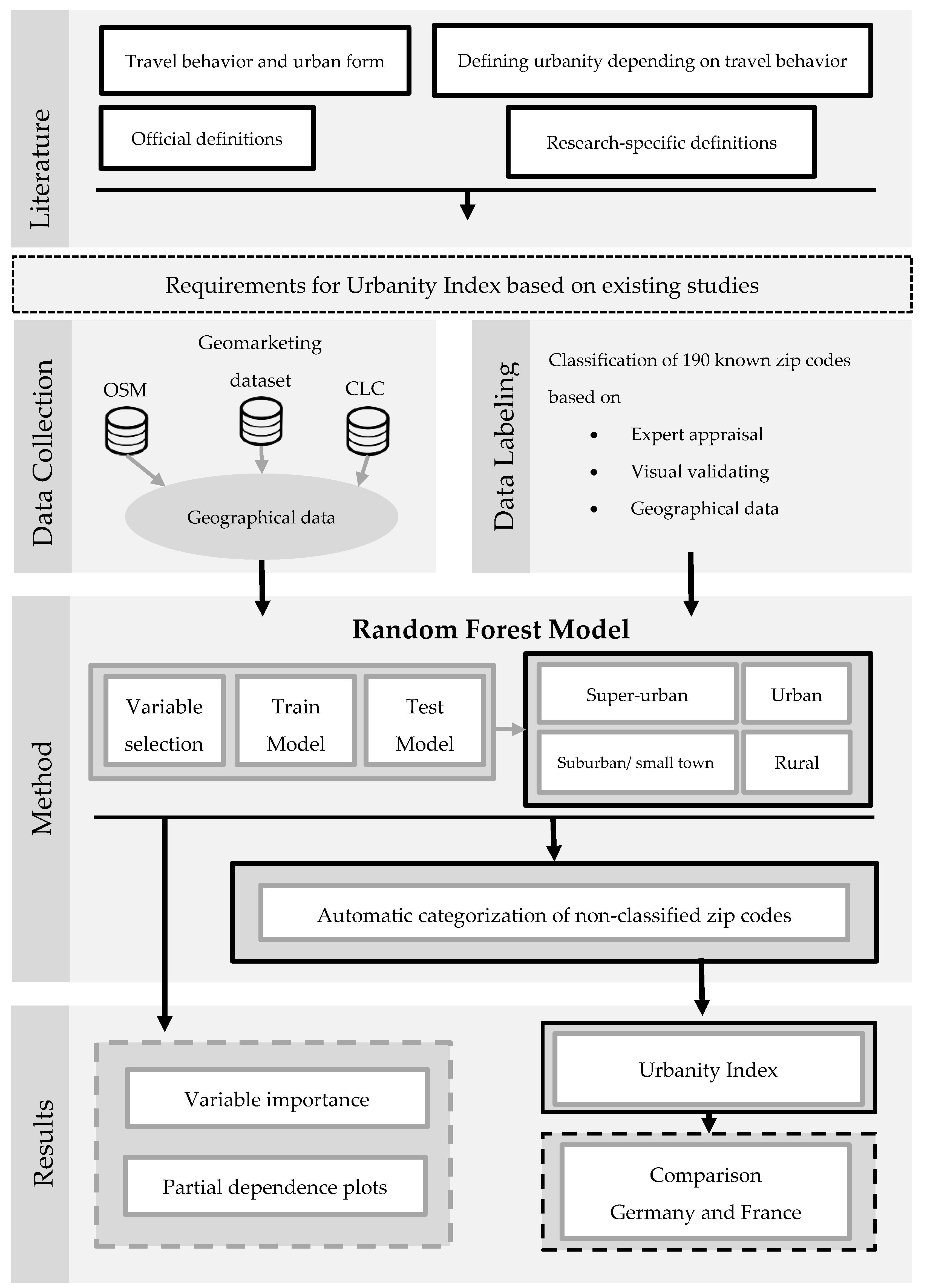
To generate the geographic data for the UI we use information concerning accessibility, diversity, and density from various sources and combine it at the zip code level. Known zip codes are then categorized by experts (transportation researchers, spatial planners, and mobility analysts) into one of the four urban categories (super-urban, urban, suburban/small town, rural).

To provide a scalable methodology the relationships between the geographical data and the categories are learned using a supervised learning technique called random forest (RF) model. It is one of the most accurate learning techniques available. For many data sets, it produces a highly accurate classifier. An RF model has several advantages over other techniques. There is no need to work with assumptions on the distribution of data or to perform extensive preprocessing of the data, e.g., transformation. In their study, Short Gianotti et al. [7] applied an RF Model to define urbanity. Unlike most other supervised learning techniques, an RF Model also provides insights for interpretation, e.g., variable importance measures (VIM). Through applying the RF model and calculating the VIMs, we are able to observe the influences of different variables on the categories and identify the most significant. The RF model is then used to automatically assign uncategorized zip codes into the four spatial categories. Using this approach after the creation of the UI, we are able to compare Germany and France using a similar definition of urbanity and aligned data sources.

The general assumption for the UI is that travel behavior differs for different area types. In rural areas, for example, there is almost no PT, which is why individuals are primarily dependent on their cars. In urban areas alternatives to the car are available and there are also many POIs accessible to meet daily needs. The UI offers the possibility of linking, e.g., vehicle sensor GPS-data with the UI and quantifying these differences. Due to international comparability, this quantification can be carried out for several other countries.

This paper is structured as follows (see Figure 1). First, we present an overview of the literature analyzing the relationships between travel behavior and different urban forms. We discuss different definitions of “urban” used by official institutions and specific research areas, and we also present existing studies in which urbanity is defined in the context of travel behavior. On this basis we define four requirements for the development of the UI. In Section 3, the approach to merge the different data sources to enable analysis of the relevant geographical data at the zip code level is described. In Section 4, we describe the labeling approach to assign zip codes into the four categories, the study methodology, and model algorithm. Finally, the influences of the different variables on the categorization as well as the comparison of data from Germany and France based on the UI are discussed, along with key implications, limitations, and opportunities for future research.

2. Literature Review

Giuliano and Narayan [1] mentioned in their study that a measure of urban form across two cities or countries is difficult due to data limitations. In

Table 1. Overview of literature in the context of defining urbanity.

Author (Year)	Study Area	Resolution	Criteria
	Defining Urbanity Depending on Travel Behavior
Motte-Baumvol et al. [8]	Paris (FR)	Municipalities	Local Inventory/POI
Siedentop et al. [10]	Stuttgart (GER)	Settlement areas	Public transport/POI
Short Gianotti et al. [7]	Boston (USA)	1 and 2.5 km2	Population, landscape
Winters et al. [11]	Vancouver (CA)	10 m2 cells	Land use, quality, availability, street connectivity
Gu et al. [13]	Chinese cities	Street segments of 50 m	Safety, convenience and comfort
Krenn et al. [12]	Graz (AT)	100 m2 cells	Infrastructure, landscape
	Research Specific Definitions
Öğdül [14]	Turkey	NUTS 4	Population, landscape
Soylu [15]	Istanbul	Neighborhood	Economic data, sociodemographic, Industrial structure
Arellano and Roca [16]	China	30 m/pixels	Night-time lights
	Official Definitions
OECD [17]	30 countries	Country specific	Population
Dijkstra and Poelman [18]	31 countries	1 km2	Population
UN [19]	200 countries	Country	Population

POI = Points of Interest; NUTS 4 = Nomenclature of Territorial Units for Statistics 4; UN = United Nations; OECD = Organization for Economic Co-operation and Development.

we present a selection of studies, taking into account the study areas, resolutions, and criteria for defining urbanity. Definitions of urban forms or built environments are often not consistent between countries or cities, leading to biased results. Motte-Baumvol et al. [8] addressed this problem and defined the degree of spatial car dependence in the outer suburbs of Paris (France) through a Local Inventory (LI) on the level of municipalities. LIs describe the number of local amenities, shops, and services and are comparable to points of interest (POI). The authors assigned the municipalities to four categories of car dependence: weak, medium, strong, and very strong. When a municipality lacks certain LIs, inhabitants are forced to travel to neighboring municipalities to acquire these. On this basis municipalities were ranked in terms of strength of car dependence. Motte-Baumvol et al. [8] concluded that in these municipalities walking is precluded by low density and the discontinuity of the urban fabric. Also, since public transit is poor, there are only a few alternatives to cars, which creates a strong spatial car dependence. This dependence is in contrast to a subjective or objective car dependence, where people like to drive a car or have certain mobility requirements such as chauffeuring their children to sport activities [9]. Municipalities with strong car dependence were characterized by greater car ownership and higher automobile mileage [8]. Siedentop et al. [10] also defined spatial car dependence in the region of Stuttgart (Germany) based on the lack of available alternatives to a car. They created an indicator concept which measured the quality of PT for each residential building as well as the accessibility of POIs with non-motorized transportation. An algorithm was used to determine the distance from each residential building to the next transportation station or POI (e.g., elementary school, doctor, or pharmacy). In addition, they evaluated the availability of PT by assessing the quality of connections to other locations. On this basis, the authors defined four categories of car dependence: very low, low-middle, middle-high, and very high. Both studies addressed the relationship between spatial structures and mobility patterns for specific regions and used four categories for car dependence. Winters et al. [11] used focus groups to develop a bikeability index based on criteria for bicycle facilities, connectivity, topography, and land use with a resolution of 10 m². With the help of the bikeability index, politics are able to identify new routes with a high bikeability score. Krenn et al. [12] also developed a bikeability index for Graz (Austria) based on infrastructure and landscape criteria (bicycle pathways, green areas, main roads, land-use mix, and topography) with a resolution of 100 m² cells. Gu et al. [13] measured walkability and bikeability in four Chinese cities (Tinjin, Chongqing, Shijiazhuang, and Kunming) using freely available Open Street Map (OSM) image data. Their study defined a bike or walk score on street level which is characterized by safety convenience and comfort.

In addition to travel behavior, existing literature also aims to define urbanity. It is important to note that under certain conditions different definitions of “urbanity” are appropriate, especially when it comes to specific research questions [7,14]. Hence, a range of studies applied different definitions of “urbanity” to different fields of research. Öğdül [14] examined Turkey based on Nomenclature of Territorial Units for Statistics 4 (NUTS4) level and used a two-step cluster analysis to divide the country into: (1) dominantly rural districts, (2) dominantly urban districts, and (3) transitional districts. Soylu [15] analyzed the instability of the urbanity in Istanbul over time and received up to seven different types of urbanity. A different approach to determine and analyze the physical change in landscape in China was provided by Arellano and Roca [16]. With a focus on spatial dynamics and sustainability, they used the number of night-time lights in a certain area to characterize urbanity. An advantage of this approach is the reproducibility due to freely available data from the U.S. Air Force Defense Meteorological Satellite Program Operational Linescan System. Short Gianotti et al. [7] analyzed urbanity in Boston (USA) from an urban ecology perspective to improve natural resource management. Their approach used an e-mail survey to investigate perceptions of “urban”, “suburban”, and “rural” of 314 landowners. With the help of a decision tree, the relationship between the perceptual definition and geospatial characteristics was identified. Other areas were then automatically divided into “urban”, “suburban”, or “rural”. The many different approaches show that a comparable definition of urbanity does not exist. This is, however, necessary to investigate urbanity in a spatial context.

In addition to these definitions of urbanity given by research studies, a number of approaches focus on nationwide investigations of urban forms published by official institutions. Here, urbanity is mainly based on population criteria. One widely established approach comes from the Organization for Economic Co-operation and Development (OECD) [17] to classify areas into predominantly urban, intermediate, and predominantly rural. Dijkstra and Poelman [18] considered a harmonized definition of urbanization based on population criteria with a resolution of 1 km² among 31 countries. The UN [19] provides annual estimates of the development of urban and rural populations for over 200 countries. Due to country-specific definitions of urbanity and inconsistent data sources, however, there is a lack of standardization of this data and direct comparison is not possible [16].

In summary, there is substantial demand for research investigating the relationship between travel behavior and spatial structures. However, there is a lack of consistent definitions of urban forms in the context of travel behavior, especially at international level. Some studies already addressed this need, however, only on regional level. In addition, approaches are often not scalable and therefore not applicable to other regions [11,12]. Other studies focus on cities and do not take rural areas into account. Therefore, it is not possible to measure differences in travel behavior between rural and urban areas. An internationally comparable approach would provide considerable practical benefits for mobility service providers or car manufacturers to understand differences in car use depending on urban forms. Specific definitions from other fields of interests tend to be very detailed and are therefore not scalable or extendable to a national or international level. Official definitions at an international level only define urban forms in terms of population criteria and do not consider factors influencing travel behavior (e.g., PT, POI, land use).

In this study we aim to contribute to the understanding of urbanity through insights on spatial mobility dependence using data comparison across different countries. To support this analysis, we approach urbanity through criteria related to car use, and develop a uniform and internationally comparable definition of urbanity based on consistent criteria and data. To generate the relevant data and ensure reproducibility, we follow Short Gianotti et al. [7] and Xu et al. [20] and use mainly open-access data, e.g., OSM.

3. Materials

As outlined in Section 2, the identification of urban structures and their forms has been the main challenge of most urban studies. Although many studies have been conducted on the identification and definition of urban levels, there is no standard definition of “urbanity” and no standard toolsets for its analysis. In particular, a comparative analysis of differences in urban forms at the cross-national and fine spatial resolution level has not been conducted. Our aim in this Section is to provide a methodological approach which enables the identification and comparison of different urban structures at zip code level across Germany and France. These two countries reflect the contrasting spatial patterns of two distinct state structures (federalism and centralism) at the European level.

One reason for the selection of zip codes as the unit of spatial analysis is due to the fact that zip codes are a common way to divide countries based on population size. In general, a consolidation of data sources at the zip code level is very suitable, also because commercially available socio-spatial datasets (e.g., marketing studies or statistics from official institutions [21]) are often delivered at the zip code level due to data privacy considerations. A UI at zip code level is flexible and can be linked to a wide variety of data. For example, Acevedo-Garcia [21] aggregated socioeconomic information at block group level to zip code level to match census demographic information with risk factors for tuberculosis in New Jersey.

3.1. Data Collection and Processing

Defining, measuring, and quantifying urban levels using internationally available and analogous datasets is the main challenge in most urban studies. The selection of appropriate datasets for this study included extensive research, exploration, evaluation, and selection of relevant databases. From this research and investigation, three main data sources for the development of the UI were selected (see Figure 1): OSM snapshots, Geomarketing dataset, and Corine Land Cover (CLC).

OSM snapshots from May to September 2018 for the selected countries of the study area were acquired freely as shapefile format from Geofabrik servers [22]. OSM provides physical elements in the landscape that can be mapped using a conceptual data model which consists of elements such as “Nodes”, “Ways”, and “Relations” [23]. “Nodes” elements define points in space by their latitude, longitude, and an identifier. “Ways” consist of an identifier and an ordered list of nodes, and define linear features and area boundaries. “Relations” are used to explain how other elements work together. Additionally, each feature includes a further list of key-value pairs called “Tags”. “Tags” describe the specific features of particular map elements. In this study we used node elements from the OSM dataset.

The digital boundaries, specifically zip code areas, are not freely available for most of the countries around the world. The commercially available Geomarketing dataset provided the digital boundaries of the study areas in shapefile format, along with complementary data on socio-demographics such as population, purchasing power (PP), and household size at the zip code level. Digital boundaries consist of administrative boundaries and depend on the country’s two- to seven-digit zip code areas. For instance, zip codes in Germany use the following system: zip codes have five digits, such as 86720, of which the first two digits indicate the geographic zone. Of these, the first digit 8 (Leitzone) stands for the region covered, namely Bavaria, and the second digit 6 (Postleitregion) stands for a zone in that region. This is similar to France, who also follow the five-digit logic. In the UK, however, a zip code consists of five to seven alphanumeric characters (including letters and numbers, like AA9A 9AA). As a result, different zip code areas have differing population sizes and areas, which necessitates further processing of data to ensure comparability.

The latest pan-European land-use land-cover (LU/LC) dataset of Corine Land Cover (CLC v.20) was acquired from Copernicus Land Monitoring Service (https://land.copernicus.eu) [24]. Jokar Arsanjani et al. [25] provide a definition of LU/LC maps as follows: “LU maps illustrate human activities, such as artificial surface construction, that represent the usage of land; whilst LC maps display the physical and biological cover over the land surface regardless of the purpose for which they are used”. Furthermore, they emphasize the important role of LU/LC datasets in various fields such as urban and regional planning and policy-making. The dataset “CLC2018” is in raster format (100 m resolution) and consists of an inventory of land cover in five main classes—(1) artificial surfaces, (2) agricultural areas, (3) forest and seminatural areas, (4) wetlands, and (5) water bodies—and 44 sub-classes (such as continuous urban fabric, industrial, commercial and transport units, open spaces with little or no vegetation etc.) [26]. In our study, we used the information on sub-classes relating to built-up areas, specifically, urban fabric, industrial-commercial areas, and transport units. The main data processing steps following data collection consisted of mostly standard geoprocessing analysis, such as selection by attributes, merging, buffer analysis, and clipping. Firstly, all datasets were imported into the GIS environment (ArcGIS 10.6) and adjusted into the standard WGS84 coordinate system. OSM data, which are represented as “nodes”, i.e., points, were filtered by means of their attributes/tags. In this way, we created data layers for accessibility related variables (bus and rail stops) and diversity related POI variables. The POI layer included categories such as retail stores, entertainment centers, restaurants, firms and companies, medical and education institutions. Afterwards, via spatial join, each point feature (stops, POIs) was counted for each polygon and saved as a new attribute for further analysis (see Section 3.2). Processing of CLC2018 datasets included conversion of raster cells to points and spatially joining these points to polygons (zip code areas), resulting in the count (i.e., area in km²) of each sub-class (urban, industrial, etc.) for each zip code area.

Overall, the raw geo-dataset for Germany and France consisted of approximately 14,250 polygon features (zip code areas) and 1.25 million node features.

3.2. Choosing the Variables to Measure Urbanity

Based on the three data sources, a range of variables was available to define urbanity. In our study we considered urban areas as consisting of different types of constructed and open spaces, i.e., buildings, transport infrastructure, green areas, water bodies, etc., and the existence, size, and shape as well as the spatial layout of these urban land covers were used to define the morphology of the area. However, urban morphology and form in themselves do not provide sufficient evidence for any direct conclusions regarding levels of urbanity. To support our analysis, we needed greater insights into the functional differentiation of various urban levels across countries and cities in order to identify specific characteristics regarding, for instance, mobility solutions. Based on the nature of our study approach we were able to identify variables with the greatest impact on the category classification (discussed in detail in Section 4). We oriented our approach to the 3Ds (density, diversity, and design) introduced by Cervero and Kockelman [27]. Here, built environment is described by the three dimensions, which in turn influence travel demand. Our assumption was that urban levels in the context of travel behavior are shaped mainly by the transport network: the higher the accessibility, density (built area, industrial share, population), and diversity (POI) of an area, the higher its level of urbanity. The variables we included overlap very well with the 3Ds by Cervero and Kockelman [27]. In order to measure the accessibility, density, and diversity of urban environments we used the previously described spatial datasets and calculated a range of spatial metrics, including PT quality, for each zip code in the study areas (see

Table 2. Description of variables to define urbanity.

	Variables	Inputs	Definition/Calculation	Data Source
		Zip code area	Total area (km2) of zip code polygon	Geomarketing dataset (2016)
Accessibility		Bus	Number of bus stations in each zip code area	OSM (2018), Geomarketing dataset (2016)
		Rail	Number of rail stations (tram, metro) in each zip code area	OSM (2018), Geomarketing dataset (2016)
	PT quality		(20 × Rail + Bus)/Zip code area, if Rail > 0 (Rail + 3 × Bus)/Zip code area, if Rail = 0
Density		Residential area	Residential area in each zip code area (km2)	CLC2018
		Industrial area	Industrial, commercial and transport in each zip code area (km2)	CLC2018
		Built-up area	Residential area + industrial area (km2)
	Built-up share		Built-up area/zip code area
	Industrial share		Industrial area/built-up area
		Population	Total population in each zip code area	Geomarketing dataset (2016)
	Population density (km2) on built-up area		Population/built-up area
Diversity		POI	Number of POIs (tags filtered to related categories) in each zip code area	OSM (2018),
	POI (km2) on built up area		POI/built-up area

After generating the datasets from the various data sources, the next step was to classify the individual zip code areas into categories.

). PT quality is a function of the number of bus and rail stations in each zip code. To take the generally better connectivity of rail stations compared to bus stations into account, we weighted rail stations with a factor of 20. If there was no rail station in a zip code area, bus stations were multiplied by a factor of 3. The stronger weighting of rail stations is in line with existing studies. For example, Scherer and Dziekan [28] were able to prove the existence of a rail factor through face-to-face interviews. They showed that rail is preferred as a means of transport over bus.

Table 2 shows the methods for determining the remaining metrics (built-up share, industrial share, population density (km²) on built-up area, and POI (km²) on built-up area). Zip code areas vary considerably in size, the more urban the area, the smaller the zip code area, and in turn large rural areas. On the one hand this is an advantage, because urban areas are often in the focus of political discussions and these areas are also presented in a more granular way. On the other hand, the different size makes comparability difficult. In order to take this into account, we standardized sizes and densities for our assessment by dividing by (built-up) area.

4. Method

In this Section we present the approach to develop the UI considering the four defined requirements (factors influencing travel behavior, comparability, reproducibility and practical application, and scalability). First, we describe the data labeling process by the expert assessments. Afterwards, we give an overview on the special features of the RF model and present the estimation results.

4.1. Data Labeling

In the official definitions of urbanity listed in Section 2, the linear separation of urban-rural areas was possible due to the low-dimensional consideration of urbanization (population criteria). Based on the five factors considered as part of this study, linear separation was no longer possible. Zip codes with a low population density but high numbers of POIs and good PT quality can be defined as “urban”, as well as zip codes with a high population density, low numbers of POIs, and low PT quality.

In addition, due to the large numbers of zip codes being assessed, manual classification was not feasible. In this study, we used expert assessments to categorize zip codes. Expert assessments are a common practice in many other research fields to identify patterns in the data. For example, Gorges at al. [29] used a similar approach in a classification problem to develop a motorcycle impact detection strategy. As part of that study, test riders categorized road maneuvers (special characteristics like crossing railroads, potholes, or kerbs) into two groups, “mild” or “severe”.

Based on the idea of Gorges et al. [29] and Short Gianotti et al. [7], the experts defined and divided well-known zip codes into four categories: super-urban, urban, suburban/small town, and rural. On the one hand, the use of four categories for labeling is based on the literature. Siedentop et al. [10] and Motte-Baumvol et al. [8] distinguished four categories in the assessment of car dependence. Short Gianotti et al. [7] used only three categories for the definition of urbanity, however, they did not divide urban areas into super-urban and urban. On the other hand, we used an explorative technique to determine three or four categories in the data. This means that before applying a supervised technique with labeled data, we tested different unsupervised hierarchical clustering techniques to explore the data. With this explorative technique we could also determine three or four categories in the data. The resulting categories from the unsupervised technique were not interpretable for further analyses. However, based on the literature analysis and the number of classes in the clustering process we decided to use four categories for the labeling process.

The labeling process was conducted during three one-day workshops (27 September 2018–30 September 2018). Ten people attended the workshops. The disciplines represented were a spatial planner from a German university (one), transportation researchers from a German Mobility Panel (MOP) (two), mobility analysts (two), experts from the field of Mobility as a Service (MaaS) (three), and experts in the field of machine learning (two) from a German Original Equipment Manufacturer (OEM). The workshop had three distinct elements. First, different approaches to define urbanity through existing literature and the collected data were presented. In the next step possible approaches to define urbanity (rule-based approach, unsupervised learning, and supervised learning through expert assessment) and their advantages and disadvantages were discussed within the workshop group. Based on this discussion and the four defined requirements (consideration of factors influencing travel behavior, comparability, reproducibility and practical application, and scalability), the approach of supervised learning by expert assessment was selected. The process of classifying zip codes was divided into two steps. First, zip codes to be classified were selected. In the second step, these zip codes were sorted according to their urbanity and divided into the four area types.

The composition of our expert team ensured the transfer from research to practical application. “Super-urban” areas represent zip codes where car use is associated with very strong pain points. In “urban” areas, traffic jams and parking search are normal. Individuals located in “suburban/small town” areas are presented with a limited availability of transportation alternatives and car users have an advantage. In “rural” areas quantity and quality of PT are very low, and people are dependent on cars.

Due to the fact that the experts were mainly based in Germany, the focus in the labeling process was on Germany, with 160 labeled zip codes. Spatial conditions in the related zip codes were established by the experts. In addition, 30 well-known zip codes across Spain (8), France (4), United Kingdom (14), and Italy (4) were allocated.

In order to reduce the subjectivity of the expert assessment as much as possible, we validated the assessment in two ways. On the one hand, we validated the results on a visual basis by looking at the zip codes and their structures in detail via GoogleMaps. On the other hand, data-based verification of the labeled zip codes was conducted with the collected data from OSM and CLC2018.

4.2. Estimation and Interpretation of the Random Forest Model

In our study we applied the supervised machine learning RF method to estimate the four area types based on the labeled data provided by expert assessments, as well as through the usage of geographical data and visual maps.

Many machine learning techniques are considered too much of a “black box”, and although they may achieve better overall results, they often lack interpretability, which, for the purposes of our study and application of the UI, was of high importance. To improve machine learning interpretability, Friedman [30] proposed the use of partial dependence plots (PDP). These are not limited to bagging algorithms but may also be applied to a wide variety of models. With this technique, the partial influence of a single variable on the classification or regression can be visualized. A well-known source of interpretation for RFs specifically is the variable importance measure (VIM), which gives a relative indicator of importance within a model. While there are many other machine learning algorithms that have been proven to be highly successful in many fields, this paper focused on the RF model. The RF model performs well with many variables, and it usually requires no complex parameter tuning to produce good results, as shown, for example, by Caruana and Niculescu-Mizil [31]. In addition, we had the ability to handle data without further pre-processing. This means we did not have to rescale, transform, or modify the data. In particular, multivariate statistical methods have stringent preconditions for application and require pre-processing of the data. The RF model has a high resistance to outliers and runs efficiently on large data sets. This characteristic is important, because in some zip codes extremely high values may occur, if, for example, a main station with an extremely high public transit density is in the zip code. For the estimation of area types in the RF model, we used the software package R and the Wright and Ziegler [32] implementation in the ‘ranger’ package, a fast C++ implementation with a clear R interface and various additional options, such as support for sparse matrices and class probability predictions. We used the standard settings of ranger to compute the predictions, except that the importance was derived by the “impurity” method. The number of trees was set to 850.

Our main study objective was to identify special characteristics (e.g., household size, PP) in the respective area types across different countries (Germany and France) by using a uniform and comparable definition. A further significant advantage by using an RF model is that it can be simply and easily scaled up across different regions and countries, without the need to verify all included zip codes manually. Furthermore, it can be used to describe the influences on the categorization of the respective geographical information for each area type.

As mentioned before, a natural and widely known source of interpretation for RFs specifically is the variable importance measure (VIM). VIM is calculated as the decrease in node impurity weighted by the probability of reaching that node:

$${{\displaystyle \sum }}_{j=1}^C{f}_i\left(1-f_i\right).$$

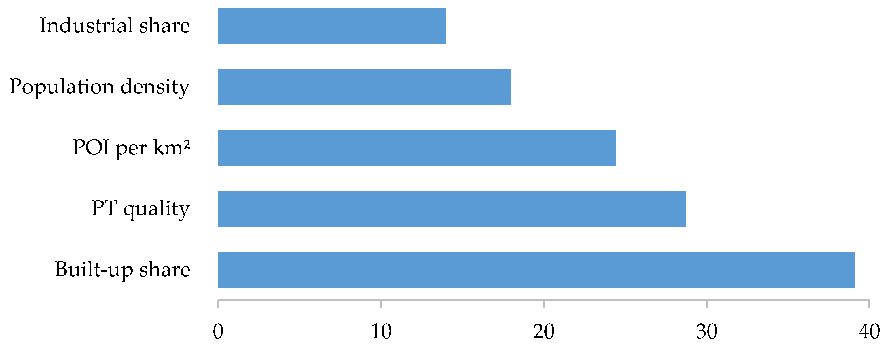
The node probability $f_i$ can be calculated by the number of samples that reach the node, divided by the total number of samples. The higher the value the more important the feature. On this basis, we first estimated a function between the categories and all included variables. Then, we used the VIM to identify the five most important variables. Each time a variable is used within a tree in the RF, the resulting two buckets become purer. Depending on the choice of impurity measure, the pureness can be defined differently. In our case, we chose the standard impurity measure of the gini coefficient. The increase in purity can be expressed through the difference of the purity before and after the split, which gives the split a measure of effectiveness. The higher the difference, the more “effective” the split. Across all trees and variables these measures were added to their respective variables, and in the final model of the UI this allowed us to compare different benefits between the variables. The higher the value of a variable, the more the variable contributed to increasing the purity within the model, and consequently to its importance to the success of the model. Values in themselves contain no real information, it is only in comparison to other variables where they become meaningful. The value of most variables will rise if the number of trees increases, and it is also affected by the number of randomly selected variables. Consequently, variable importance measure values cannot be compared between different models, only their order within the different models. Based on the data collection described above, a wide range of variables was available for the classification process. The relationship between the labels (190 zip codes) and the geographical data (PT quality, built-up share, industrial share, population density in built-up area, and POI (km²) in built-up area) was identified as the variable with the most influence by the RF model. The VIM of the final classification (see Figure 2) indicates the highest influence of “built-up share”. The second most important variable was “PT quality”, which considers existing alternatives to a car and describes car dependence in the zip code. The third most important VIM was “POI per km²” in the zip code. This variable represents the development of an area and whether people have to leave their zip code for activities such as shopping. The fourth most important variable was “population density”, which is used in many studies as a proxy for urbanity, and our results demonstrate potential overestimation of the influence of this variable in describing urbanity. The fifth most import variable was “industrial share”.

Compared to other machine learning algorithms the Random Forest model has a very high explanatory value and can well reflect the influence of variables on the classification. Friedman [30] and Zhao and Hastie [33] proposed in their studies the use of partial dependence plots (PDP). With this technique, the partial influence of a single variable on the classification can be visualized [33].

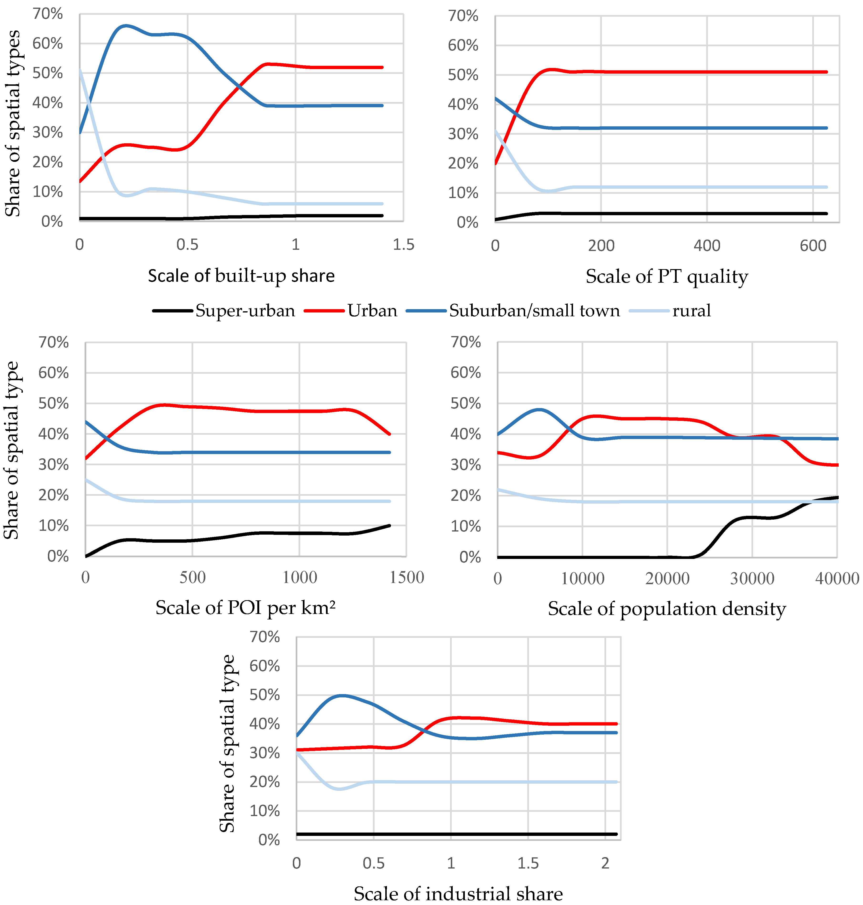
Correlations between geographical data and spatial type classification are shown in the partial dependence plots (PDP) in Figure 3. With the “built-up share” it is clear that at the beginning the “rural” type predominates. It is replaced by the “suburban/small town” type with an increasing share in the total area. The “urban” type only dominates when the share is high. This means that the zip code has a very high built-up share. In contrast, PT quality and POI are urban phenomena. Only “suburban/small town” areas prevail at the beginning and continue to play a further role with increasing POIs. “Suburban/small town” areas in particular generally have POIs at their center. When considering population density over 20,000, the strong increase in the “super-urban” spatial type is particularly evident and a shift occurs from “urban” to “super-urban”. In addition, “suburban/small town” areas with a high population density are generally housing estates without good PT access or diversity with POIs.

Error was estimated internally, during the run each tree was generated with a different bootstrap sample from the original data [34]. To evaluate the accuracy of the RF model, we looked at the out-of-bag (OOB) error. OOB error is computed by averaging trees corresponding to bootstrap samples in which observations were not used for learning. This metric is very similar to N-fold cross-validation. The stabilized model showed a suitably good OOB of 16.32%. This error is the mean prediction error for each training sample and can be used for verification.

5. Results

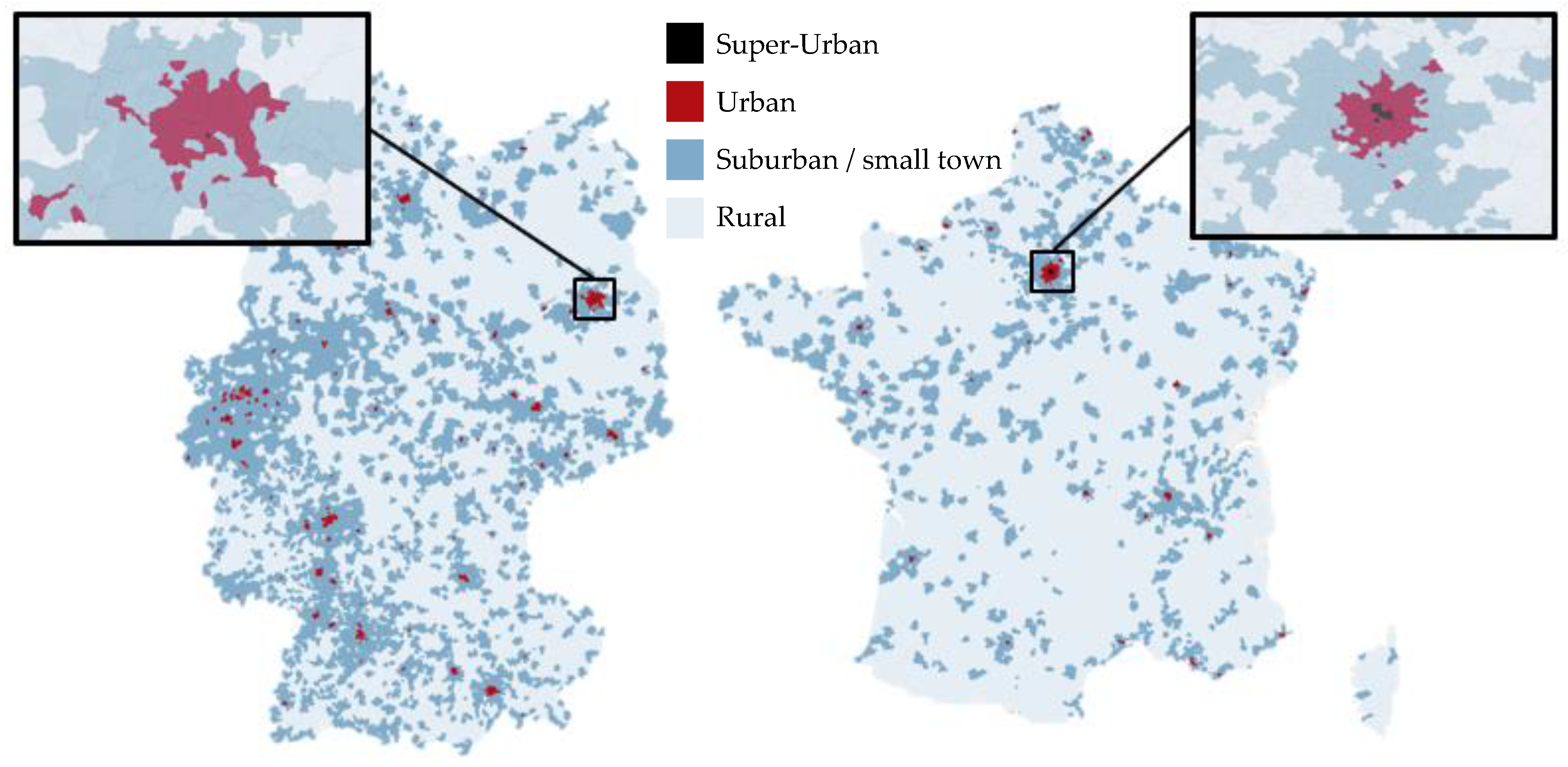
With the help of the UI we were then able to compare the urbanity of Germany and France based on population, household size, PP, car ownership, and affinity frequent driver. Data are visualized for Germany and France in Figure 4 below.

In Figure 4, black polygons represent the “super-urban” zip codes. In Germany only one zip code in Berlin was identified as “super-urban”, while in France seven Arrondissements in Paris were identified as “super-urban”. The “urban” areas, marked as red, are more evenly spread over the whole country in Germany, while in France “urban” areas are mostly located near Paris (105 out of 189 zip codes).

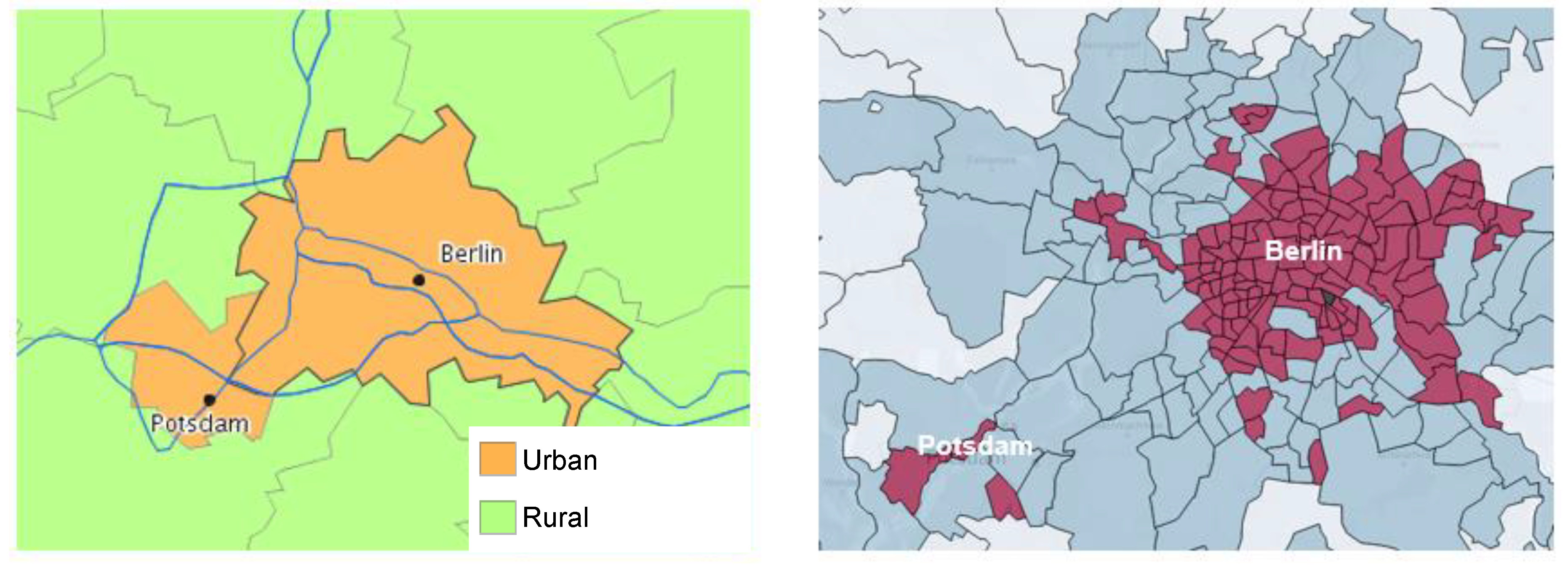
If we compare the UI with other area type typologies using a city like Berlin as an example, the advantage of the UI becomes clear. The Federal Institute for Research on Building, Urban Affairs, and Spatial Development (BBSR) conducts a continuous ongoing spatial observation project at city and communal level in Germany. Findings of this project show the living conditions at district and community level, which are then used, for instance, to evaluate national development policies and the regional distribution of federal financial resources. It is the most common resource for spatial categorization in Germany and delivers information on spatial classification varying between city, community, and regional level. However, for our research purposes, the classification of BBSR is of limited use. First of all, the finest spatial unit in BBSR is at community level (Gemeinde), which does not allow us to conclude on the intra-urban structures. While the BBSR declares Berlin as one big urban area, the UI has a more detailed view and considers Berlin as a composition of 191 zip codes (administrative areas), which include super-urban, urban, suburban/small town, as well as rural areas (see Figure 5). Secondly, the BBSR distinguishes between two types of areas (urban and rural areas), while the UI distinguishes between four area types. Finally, the typology of the BBSR is only available for Germany and is therefore not applicable in an international comparison. However, we used the population and area distribution of spatial categorizations of the BBSR to validate the distributions used in the UI. With the BBSR definition, 69% of the area is declared as rural and 32% of the population live in rural areas, while with the UI definition, 68% of the area is declared as rural and 28% of the population live in rural areas. Thus, the results are quite comparable despite different approaches.

It is also evident that “rural” areas in France are much larger than in Germany, and in Germany “suburban/small town” areas dominate the map. This assessment is also reflected by the cluster-forming variables in

Table 3. Description of cluster-forming Variables of Germany and France.

	Used Variables to Define Urbanity
Area Types	PT Quality (StDev)	Built-Up Share (%) (StDev)	Industrial Share (%) (StDev)	Population Density (km2) on Built-Up Area (StDev)	POI (km2) on Built-Up Area (StDev)
	Germany
Super-urban	49.4 (-)	1.0 (-)	0.00 (-)	28,747 (-)	480.0 (-)
Urban	83.6 (72.5)	0.8 (0.2)	0.44 (1.95)	9268 (4902)	203.9 (753,0)
Suburban/small town	8.0 (10.5)	0.3 (0.2)	0.28 (0.53)	3037 (1363)	25.1 (61,9)
Rural	1.4 (1.2)	0.1 (0.0)	0.08 (0.21)	2241 (1239)	14.7 (20,9)
Average	9.8 (29.1)	0.2 (0.2)	0.18	3043 (2542)	32.2 (210,7)
	France
Super-urban	122.8 (41.7)	0.9 (0.1)	0.01 (0.02)	33,229 (5905)	526.6 (213,0)
Urban	50.2 (33.2)	0.8 (0.1)	0.39 (1.18)	11,524 (6777)	110.3 (156,0)
Suburban/small town	6.5 (8.3)	0.3 (0.2)	0.30 (0.39)	2465 (1356)	11.0 (11,8)
Rural	0.4 (0.8)	0.1 (0.1)	0.08 (0.21)	2058 (1558)	11.2 (19,0)
Average	3.8 (12.05)	0.2 (0.2)	0.15	2496 (2687)	14.7 (40,5)

. The number in brackets represents the standard deviation (StDev) of the respective variable. Considering the min/max values of the variables, the advantage of non-linear structures becomes apparent. The minimum and maximum value of the population density on built-up areas in Germany is 0 and 33,036 in urban areas and 160 and 16,073 in suburban/small-town areas. Thus, areas were declared as urban which have a very low population density on their built-up area, but at the same time other variables have a very high value. The population density for built-up areas on average is 3043 (2542) in Germany and 2496 (2687) in France per km² of built-up area. As expected, population density increases in both countries with the degree of urbanity. Within the “urban” and “super-urban” areas, France is on average denser. In Germany, the density is higher in “suburban/small town” areas. The break-down in Germany is mainly based on spatial planning analysis through the application of the central place theory, which describes and limits the settlement structure. Small towns assume a central local function and become denser as a result. This also becomes clear when comparing POIs per km² in built-up areas. Fewer POIs also means that people are more dependent on their cars, as they have to travel longer distances to get around [8]. The “built-up share” also rises with urbanity. Urban areas have a high proportion of built-up areas and differ from less densely built-up spatial types. As shown in the VIM values, “built-up share” is an important distinguishing characteristic. The “industrial share” is lower in “suburban/small town” areas, as these are often not mixed, but rather purely residential. In urban areas in France and Germany, mixed use areas can also be observed to an increasing extent, as reflected by specific provisions in building planning laws. A strong difference between France and Germany can be seen when comparing the quality of PT. Apart from the “super-urban” values, “PT quality” in Germany is, on average, higher. This is also due to the high availability of rail PT. When assessing dependence on cars, it is evident that people in Germany have better alternatives to cars than in France, and consequently they have a lower spatial car dependence [10]. In rural areas there is almost no PT available in France, whereas in Germany, basic services are often provided.

Furthermore, the more rural, the larger the average size (km²) of the zip codes for both countries (GER: super-urban: 0.5, urban 2.7, suburban/small town: 23.1, rural: 35.3; FR: super-urban: 2.9, urban: 5.5, suburban/small town: 21.6, rural: 96.7 km²).

The distribution of the population and average PP among the four area types also show differences between Germany and France (see

Table 4. Population distribution, purchasing power, average household size, car per 1000 inhabitants and affinity frequent driver by area types and country.

	Country
	Germany			France
Area Types	Population Share	Purchasing Power		Population Share		Purchasing Power
Super-urban	0%	17,967 €		1%		28,987 €
Urban	13%	22,235 €		15%		22,128 €
Suburban/Small town	59%	22,512 €		46%		20,060 €
Rural	28%	21,388 €		37%		17,856 €
Average	-	21,025 €		-		22,258 €
Area Types	Household Size	Cars Per 1000 Inhabitants	Affinity Frequent Driver	Household Size	Cars Per 1000 Inhabitants	Affinity Frequent Driver
Super-urban	1.67	169	81.33	1.84	222	82.59
Urban	1.72	562	88.59	2.20	390	88.08
Suburban/Small town	2.05	569	101.65	2.37	530	108.25
Rural	2.25	633	107.51	2.33	555	99.83
Average	1.92	604	100	2.19	543	100

). Almost 60% of the German population lives in the “suburban/small town” area type, while in France this is only 46%. This difference is distributed mainly among “rural” areas (GER: 28%, FR: 37%), and slightly among “urban” areas (GER: 13%, FR: 15%). The high proportion of “rural” areas in France can be seen in the visual analysis of the countries (see Figure 4) and is confirmed by the distribution of the population by area type. The PP analysis also revealed important differences. A more affluent populace lives in the “super-urban” neighborhoods in Paris, and in France in general PP increases with urbanity, which is also strongly marked by centralism and a larger number of higher salary jobs. In Germany, the PP between the different area types is almost identical. The assessment of “super-urban” areas was not included, as in Germany there is only one and in France only seven zip code areas identified as “super-urban” in the UI. A major strength of the UI is demonstrated through the following analysis. Due to using the zip code as the primary key, any information associated with the zip code can be linked through the UI. Data were collected describing average household size, average cars per 1000 inhabitants, and average affinity of frequent drivers (FD). Using zip code areas, this information was linked to the UI and the average values for each area type was calculated. In relation to household size there is also a number of key differences. While the average household size in Germany is lowest in “super-urban” areas (1.67) and highest in “rural” areas (2.25), the household size in France is lowest in “super-urban” areas and highest in “suburban/small town” areas (2.37). Motorization in both countries declines with urbanity, although in Germany there is almost no discernible difference on average between “urban” (562) and “suburban/small town” (569) areas. In France, motorization is much lower at 390 in “urban” areas. It is also interesting to note that motorization in Germany is, on average, higher than in France. The FD value describes the affinity of frequent drivers with a car in the different zip code areas. A value of 110 means that the affinity for frequent drivers in this region is 10% above the national average. For this reason, the variable is only comparable within countries, and a meaningful comparison between the countries is not possible. One interesting point is the high value of affinity frequent driver in the “suburban/small town” areas in France. This may be due to the lack of central local function, and people needing to travel longer distances. In Germany, in contrast, the value of affinity frequent driver is highest in “rural” areas. Here, dependence on cars is also very high. These areas have connections to local sub-centers at a reasonable distance, and so the more frequent use of cars makes sense, even if there is a high degree of dependence. Many rural areas in France are isolated such that regular commuting to larger towns is not an option.

6. Conclusions

In this study we presented an approach to investigate urbanity in the context of travel behavior. Attention was given to the consideration factors influencing travel behavior (PT density, POI, composition of zip code), international comparability (uniform definition of urbanity and data base), reproducibility and practical application (open-source data, zip code level). The expert assessment and the adaptation of the RF model provided a scalable methodology for the automated assessment of the level of urbanity of different areas.

We also showed additional approaches for the analysis of RF models, and used two methods for analyzing results: VIM and PDP. Both methods contributed to the understanding of influences on the allocation process, and the results from the PDP show that RF models can handle non-linearity without requiring further adjustments. The UI presumed a higher population share in “suburban/small town” areas in Germany than in France. The better access to PT and higher density of POIs in Germany has a number of consequences. Individuals can be more flexible in their travel behavior and can choose more easily between public and private transport. This also simplifies any transition to environmentally-friendly transport alternatives. “Rural” areas tend to have greater car dependence, which means individuals depend on their private transport and cannot easily switch between public and private transport. In countries such as France, the transition to environmentally-friendly transport alternatives could be made more difficult by the relatively high proportion of “rural” areas compared to Germany. The UI and the related logic offers tremendous possibilities to link different data sources (e.g., sociodemographic data) on the basis of zip codes, but also has some limitations:

• Zip codes represent a combination of letters and digits within postal addresses in order to define the delivery location of a letter or a package. This logic is established in western countries, but not in China, for example. The UI and its zip code logic could therefore only be applied to such countries with data quality limitations;
• The required data for assessment were primarily obtained from OSM and CLC, however, the actuality and quality of the data can differ from country to country. This makes a homogeneous comparison on uniform database difficult, particularly in the case of countries undergoing major structural change.

The current design of the UI offers opportunities for further development and new insights:

• OSM and CLC data only provide information on where there is access to PT, no information is available regarding PT stop frequency. Stop frequency has an influence on the quality and attractiveness of PT and should be considered in future research;
• Car commuting can be used to determine interaction between zip codes. In combination with the UI, new insights could be gained concerning differences in car commuting between different area types, thus optimizing the design of mobility solutions (e.g., defining relevant ODM areas or implementing charging infrastructure) in the respective areas;
• The attitude towards different types of vehicles and the openness to different means of transport with alternative propulsion systems (e.g., electric vehicles) can be analyzed to determine, for example, whether people in urban areas are more open about alternative propulsion systems;
• A further indicator to extend the UI would be the consideration of the electric vehicle utilization rate in a certain area. The greater the electrification, the more urban the area [35].

In conclusion, a flexible and homogenous international comparison of urbanity is important in identifying key differences in urbanity, and developing designs for new mobility solutions and more environmentally-friendly means of transport which meet the specific, individual needs within the situation of a city or a country. Based on the UI, policies and their impact could be transferred to other countries, as the UI makes areas comparable, regardless of the country. This would have a great potential for savings, as not every country has to pilot political measures.