Finite Element Method for the Estimation of Insertion Loss of Noise Barriers: Comparison with Various Formulae (2D)


1
Institute of Computational Mechanics and Optimization (Co.Mec.O), School of Production Engineering and Management, Technical University of Crete, 73100 Chania, Greece
2
Department of Music Technology and Acoustics, Hellenic Mediterranean University, 74100 Rethymno, Greece
*
Author to whom correspondence should be addressed.
Urban Sci. 2020, 4(4), 77; https://0-doi-org.brum.beds.ac.uk/10.3390/urbansci4040077
Submission received: 25 September 2020
/
Revised: 21 November 2020
/
Accepted: 17 December 2020
/
Published: 21 December 2020
(This article belongs to the Collection Urban Acoustic Environments)
Abstract
:Noise barriers are a critical part of noise mitigation in urban and rural areas. In this study, a comparison of the insertion loss calculations of noise barriers via the Finite Element Method (FEM) and various formulae (Kurze–Anderson, ISO 9613-2/Tatge, Menounou) is presented in the case of two-dimensional acoustic radiation problems. Some of the cases explored include: receiver in the illuminated zone, in the shadow zone, in the shadow border, source in medium, long, short distance from the barrier, source and receiver near barrier, and source above the barrier. Comparisons of the results indicate that FEM results comply well (less than 1 dB in each case) with Menounou’s formula which in turn complies with the analytic solution (MacDonald Solution). In certain cases, the differences between FEM and Menounou’s formula compared to Kurze–Anderson and ISO 9613-2/Tatge formulae are substantial (source and receiver near the barrier (10 dB) and source near the barrier and receiver in the shadow border (5 dB)). Similar differences are also confirmed by the analytic solution. The findings suggest that FEM can be applied effectively for the precise estimation of the insertion loss of noise barriers. Especially in cases where ISO 9613-2 formula shows large deviations from the analytic solution (e.g., near barrier), possible applications may arise in cases such as balconies, facades, etc. Furthermore, the study supports the idea that FEM could possibly be effectively utilized in real life applications for microscale urban acoustic modeling as a viable alternative to expensive noise prediction software.
1. Introduction
A noise barrier can be considered as any solid obstacle that impedes the line of sight between the source and receiver and thus creates a sound shadow [1]. Noise barriers are an important aspect of fighting noise pollution both in urban and rural areas caused by major infrastructure projects such as roads, railways, and airports. In the context of improving the urban environment and in order to meet recommended guideline values for community noise (e.g., World Health Organization (WHO) [2]), implementing noise barriers is one of the most used and effective methods.
Noise barriers come in many forms and shapes. The use of numerical methods is of great importance in their development as well as in the evaluation of their effectiveness. We can mention barriers with diffracting edge modifications such as T-shaped barriers [3], multiple-edge barriers [4], Y-shaped [5], with tubular cappings [6], with fir-tree profile [7], with passive phase interference devices [8], and with absorptive treatment [9,10]. Other forms include earth mounds [11], cantilevered and galleried barriers [12], picket [13] and louvered barriers [14], sloped [15] and dispersive barriers [16], barriers with vegetation [17], biobarriers [17], sonic crystals [18], barriers that fight air pollution [17], exploit solar energy [17], with active noise control [19], and barriers that are used for energy harvesting [20]. Noise barriers can be made with a range of materials including timber, sheet-metal, concrete, brick, plastic, PVC, and fiberglass [17]. The optimization of barriers has also been applied through scaled experiments [21], genetic algorithms [22], topology optimization [23,24], and artificial neural networks [25]. For a more detailed description, the reader can refer to [1,17,26]. Also, it must be noted that noise barriers are also used indoors e.g., in open plan offices (usually named as screen barriers or acoustic screens) [27,28,29].
The main phenomenon characterizing the acoustic behavior of a noise barrier is diffraction, while absorption and transmission are also important. The performance of a noise barrier is measured by insertion loss which is defined in ISO 9613-2 [30] as: ‘difference, in decibels, between the sound pressure levels at a receiver in a specified position under two conditions: (a) with the barrier removed, and (b) with the barrier present (inserted), and no other significant changes that affect the propagation of sound’. However, it must be noted that the effectiveness of a noise barrier regarding its perceived loudness attenuation is also affected by its visual characteristics [31,32].
1.1. Mathematical Formulation, Exact Solutions and Approximate Analytical Solutions
The first mathematically formulation for the diffraction of a plane wave by a semi-infinite plane screen was given by Sommerfeld [33]. Thereafter, MacDonald [34] developed a solution in a spherical polar coordinate system that was subsequently recast in the cylindrical polar system by Bowman and Senior [35]. An accurate integral representation of the diffracted wave from a semi-infinite wedge has been given by Hadden and Pierce [36].
Many approximate analytical solutions for diffraction by a half plane can be found such as the Fresnel–Kirchhoff approximation [37] and in studies by Rubinowicz [38] and Embleton [39], with the former being the most common one. The Fresnel–Kirchhoff approximation is a mathematical representation of the Huygens–Fresnel principle which is in wide use in optics. In this approximation the Helmholtz equation is solved with the aid of Greens theorem. The sound pressure at a receiver can be written as an integral to be evaluated over a surface of infinite extent. An extensive overview of all the above can be found in the study by Li and Wong [40].
1.2. Formulae of Insertion Loss
Simple formulae and charts [37,38,39,40,41] are proposed for the calculation of insertion loss of semi-infinite noise barriers, since exact and approximate solutions are not easily applicable for engineering purposes and software implementations due to their mathematical complexity.
The first known attempt was developed by Redfearn [41], while Maekawa [42] presented the most influential work. Maekawa, in his study, used pulsed tones of short duration to measure the attenuation of a thin, rigid barrier, for different source and receiver positions. The results were presented in a chart where the attenuation was plotted against a single parameter known as the Fresnel number (numerical ratio of the path difference between the diffracted path and the direct path of sound to the half of a sound wavelength). In the same period, Rathe [43] also presented an empirical table for sound attenuation by a thin, rigid barrier due to a point source.
A well-known formula for calculation of insertion loss is that of Kurze and Anderson [44,45] which is referred in most relevant textbooks [1,17]. In their work, Kurze and Anderson reviewed diffraction theory from Keller [29] and used Maekawa’s and Redfearn’s experimental data to derive a simple formula for barrier attenuation.
Another simple formula that fits the Maekawa data quite well is that of Tatge [46] which can also be found in ISO 9613-2 [30] (case for single diffraction, no ground reflections). The importance of this equation lies in the fact that various sound mapping software comply with ISO 9613-2 requirements.
More recently, Menounou [47] presented a new, optimized formula as a correction to the Kurze–Anderson formula. In her study, a comparison of the results between Maekawa’s curve and the MacDonald solution [33] was presented, especially for configurations where both source and receiver were close to the barrier and where the receiver was at the shadow border (the line where the barrier nearly breaks the line of sight between the source and the receiver). Discrepancies, 15 dB and 3 dB, respectively, were observed. Similar experimental results, in agreement with the MacDonald solution but with a great deviation from Maekawa’s curve, were reported by Kawai et al. [48] in the case when either the source or the receiver is comparatively near the barrier. The same conclusion was also reported by Hu and Wong [49]. The goal of Menounou’s work was to bridge the Maekawa’s curve and the Kurze–Anderson formula with the exact solutions by providing a simple and accurate formula with results similar to the analytical solution.
1.3. FEM, Other Numerical Methods and Noise Barriers
Numerical methods such as Finite Element Method (FEM), Boundary Element Method (BEM), Finite Difference Time Domain (FDTD) method, and Pseudo Spectral Time Domain (PSTD) method have also been applied for noise barriers. FEM has been used for studies for the estimation of the reflection index of multiple acoustic layered noise barriers [50], for modeling of the acoustic performance of sonic crystals [51,52,53], for topology optimization [24,54,55], for the investigation of the structural performance of a noise barrier [56], and for calculation of insertion loss [57]. However, it seems that more numerical studies have used BEM, for modeling of noise barriers with various shapes and configurations [58,59,60,61,62,63,64,65] and for barrier optimization [66,67,68,69]. The FDTD and PSTD methods have been applied for studies to a much lesser extent, [70,71,72,73] and [74,75] respectively.
FEM is probably one of the most (or the most) widely used numerical method with many software implementations and has been applied for modeling of wave phenomena in acoustics for various applications (e.g., room acoustics [76]). It can simultaneously incorporate the effects of diffraction, absorption, and transmission both in the frequency and time domains [77]. However, despite its widespread use, fewer studies have utilized FEM for studying noise barriers compared to BEM even though both methods allow any kind of shape and impedance condition values on the surfaces of the barrier. Probably, this is due to the fact that BEM appears more appropriate in an infinite space than FEM, because only the surface of the domain boundary must be discretized. However, studies show that the computational cost of the methods in exterior problems can be competitive [78] and for the same domain FEM computational cost can be lower than BEM [79]. This study supports the notion that FEM is suitable for noise barrier research and probably for urban acoustic modeling as it will be discussed in Section 4 of this paper.
1.4. Aims and Novelties
The aims of this study are to:
- Validate of the accuracy of FEM for calculation of insertion loss of noise barriers.
- Present a simple and applicable methodology for the accurate calculation of insertion loss utilizing commercial software which can be extended to various cases (e.g., predict the behavior of noise barriers with various shapes, with a profile which absorbs or disperses sound, in 3D space, etc.).
- Lay the groundwork for application of FEM for urban acoustic microscale modeling.
The novelties of this study, in relation to earlier publications, can be considered to consist of the following points:
- To the best of our knowledge this is the first study that extensively compares insertion loss results of FEM with Kurze–Anderson, ISO 9316-2/Tatge and Menounou formulae results.
- This is the first study to present the accuracy of FEM for the calculation of insertion loss of noise barriers especially in the cases where the receiver is near the barrier or in the shadow border and when both source and receiver are near the barrier.
This paper is organized as follows. Section 2 presents the methodology employed for FEM, relevant information regarding insertion loss, and the various formulae used in the study. Section 3 presents the findings of the research, while the Section 4 analyses the data, addresses the research questions, and identifies areas for further research. Finally, Section 5 gives a brief summary and contextualizes the study.
2. Methods
The section begins with an introduction to the subject of insertion loss, containing all the relevant information necessary for the next chapters. Thereafter, the FEM setup and methodology applied for the calculation of insertion loss is presented as well as the formulae that were used in this study.
2.1. Elements Regarding Insertion Loss
Elements that are going to be presented regarding insertion loss and noise barriers are: definitions, basic terminology, coordinate system, and equations that were used throughout the text.
As stated in the introduction, insertion loss is defined as: ‘difference, in decibels, between the sound pressure levels at a receiver in a specified position under two conditions: (a) with the barrier removed, and (b) with the barrier present (inserted), and no other significant changes that affect the propagation of sound’ [30]. Therefore, insertion loss can be expressed as Equation (1):
where , and , are the sound pressure levels and the acoustic pressures measured at the same location before and after the insertion of a noise barrier.
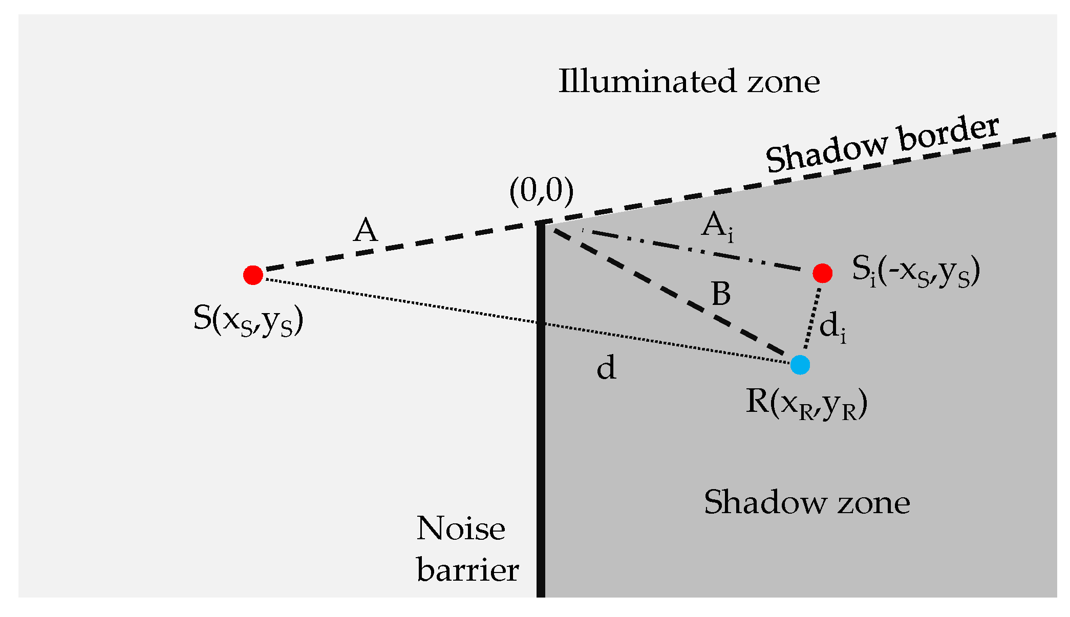
Areas around the noise barrier can be divided into zones (Figure 1). The shadow zone is the area where the barrier breaks the line of sight between source and receiver, while in the illuminated zone there is a direct line of sight between source and receiver. The shadow border is the line between the shadow zone and the illuminated zone. For a thorough mathematic description of the different regions the reader can refer to [40,80].
The theory developed for noise barriers [42] calculates the acoustic performance in terms of the Fresnel number , which is defined as:
where is the wavelength of sound in air and is the path length difference (diffracted path length minus direct path length), which can be defined as:
is the shortest path over the edge, from the source to the receiver in the barrier shadow zone, is the direct path distance between source and receiver, through the barrier. The path length difference is positive in the shadow zone of the barrier and negative in the illuminated zone.
A rectangular coordinate system with its origin at the intersection of the diffracted ray and the top edge is going to be used throughout the text, which is particularly convenient for the software implementations (for FEM and formulae). The rectangular coordinate system can also be used in 3D [44]. Subscripts S and R identify the coordinates of the source and receiver positions respectively. Therefore, , and can be defined as:
The parameter , introduced by Menounou [47], can be thought of as a second Fresnel number that is associated with the relative position of the image source to the barrier and the receiver. It is defined as the extra distance sound travels from the image source to the receiver after diffraction by the barrier edge, normalized by half the wavelength of the incident wave [47].
2.2. Formulae for the Calculation of Insertion Loss
The formulae that were used for the calculation of insertion loss are Kurze–Anderson, ISO 9613-2/Tatge and Menounou. The software Matlab v. R2015a (Mathworks, Natick, MA, USA) was used for the calculations.
2.2.1. Kurze–Anderson Formula
As stated in the introduction, probably the most well-known formula for calculation of insertion loss, which is in good agreement with Maekawa’s curve [42], is that of Kurze and Anderson [44,45]. If we assume that the sound is emitted by a point source and the barrier can be considered to be thin and infinitely long, then the insertion loss can be calculated by the following equation:
2.2.2. ISO 9613-2/Tatge Formulae
Tatge, in his study [46], presented a formulae that fits well with the Maekawa curve [42]. The formula is applied for . The same formula can be found in ISO 9613-2 [30] (case for single diffraction, no ground reflections). However, in the ISO it is stated that: ‘For large distances and high barriers, the insertion loss calculated (by the formula) is not sufficiently confirmed by the measurements’. The importance of this equation lies in the fact that various sound mapping software comply with ISO 9613-2 requirements. The ISO 9613-2/Tatge formula is expressed as:
2.2.3. Menounou Formula
Menounou, in her work [47], presented the following formula (Equation (10)) as an improvement to the Kurze–Anderson formula. As discussed in the introduction, Maekawa’s curve and Kurze–Anderson formula give predictions that deviate largely from experimental data and analytical solutions when the source or receiver is very close to the barrier surface, or when the receiver is very close to or at the shadow border.
The first term of Menounou’s formula (nomenclature of the study will be used), ILs, is a function of N1, which is a measure of the relative position of the receiver to the source. The second term is a function of N2/N1, which is a measure of the proximity of either the source or the receiver to the barrier surface. The third term is appreciable and needs to be computed only when N1 is very small, which in turn is a measure of the proximity of the receiver to the shadow border. Finally, the fourth term, ILsp, is a term that depends on the type of incident radiation and is a function of the ratio (A + B)/d. The Menunu formula is:
where:
2.3. FEM Setup and Methodology for the Calculation of Insertion Loss
Elements that are going to be presented regarding FEM setup and methodology for the calculation of insertion loss are: models created, mesh creation, and the modeling of the open pressure acoustic domain through a Perfectly Matched Layer (PML), FEM formulation.
2.3.1. FEM Models
Two models were created: for the first one the sound pressure at the receiver point was calculated without the presence of a sound barrier and for the second one with a sound barrier for the same source position. The insertion loss was calculated as the difference in sound level at receiver location with and without the presence of a noise barrier. The point source and receiver positions in relation to the sound barrier are presented in Figure 1.
For the mesh creation the rule of thumb λ/h = 5 was applied where λ and h respectively denote wavelength of upper limit frequency and the maximum nodal distance. Five elements per wavelength are typical [81] for acoustic modeling in the frequency domain, while different considerations apply for modeling in the time domain [82]. The domain was discretized with an unstructured mesh of quadratic Lagrange triangular elements. The Delaunay triangulation [83] was used in this study for automatic mesh generation. The highest frequency considered in this study was 500 Hz. The maximum element sized used was approximately 0.1 m while the minimum element size was 0.004 m. The number of total elements used was 926,958.
For modeling the open pressure acoustic domain (Sommerfeld radiation condition [84]) an appropriate Absorbing Boundary Condition (ABC) had to be applied. The Perfectly Matched Layer (PML) was used which is considered to be one of the best ABC available (for a review of ABC’s the reader can refer to [85,86]). The PML is an approximation methodology originally developed by Berenger [87] and later applied in the field of acoustics [88]. The key property of a PML, that distinguishes it from an ordinary absorbing material, is that it is designed so that waves incident upon the PML from a non-PML medium are absorbed without any (or better minimum) reflections at any frequency and at any incidence angle.
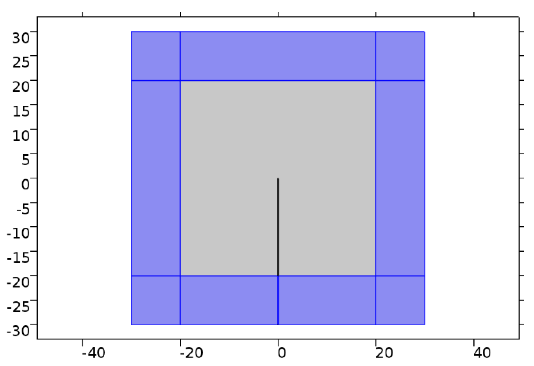
However, it must be noted that the performance of a PML is not perfect. Berenger, in his study, [87] stated that ‘small amount of numerical reflection occurs in practical computations, but with a magnitude that can be reduced by tuning some parameters of the layer, especially its thickness’. In his research, Zampolli et al. [89] (utilizing the same software as this research), used PMLs with different layers of quadratic elements (3, 6, and 12 layers). It was found that PMLs suffer from inaccuracies at very low frequencies in the case a small number of layers used. For this study, the thickness of the PML was chosen so that it consists of a larger number of layers than the maximum studied by Zampolli so that there are no (or minimum) reflections. As can be seen in, e.g., Figure 2, Figure 3 and Figure 4, a 10 m thickness was used for the PML, which with a maximum element size of 0.1 m and an unstructured mesh, resulted in a number of layers approximately between 140 and 165.
The FEM model with the PML is presented in Figure 2. The specific geometry of the PML area was chosen as it has been used in other studies [87,88] and successfully in the past by the authors [90], while other geometries can probably be used (e.g., circular). The same type of element was used in the whole domain (however hybrid meshes have been used for the same purpose-triangular elements for the main domain and rectangles for the PML [91]).
In this study the commercial software Comsol Multiphysics v.5.1. (Comsol inc., Burlington, VT, USA) was utilized for the 2D sound field models.
2.3.2. FEM Formulation
For the Helmholtz equation, p is the acoustic pressure, is the Laplacian operator, is the wave number and is given by:
The normal fluid particle velocity is related to the normal derivative of the acoustic pressure in the frequency domain by:
where represents an outward normal vector at a field point , is the derivative in the normal direction, is the angular frequency, and is the average density of the fluid.
By introducing a weak formulation with weighting function , the Helmholtz equation is transformed as follows [92]:
where and are the domain and boundary respectively. The physical quantities (acoustic pressure and particle velocity) in a discretized domain are respectively given by [92]:
where and correspond to the discrete acoustic pressure and fluid particle velocity at point . is a basis function. Substituting Equation (18) into Equation (17) and considering source terms yields [92]:
where , and are the stiffness, damping and mass matrices of the acoustic domain, respectively. The excitation vector represents the source and the pressure vector, represents the sound pressure values at the nodal locations in the acoustic domain.
3. Results
In this section, we present results from the application of FEM as well as various formulae regarding the acoustic behavior of noise barriers. Initially, the results of FEM for sound pressure levels and acoustic pressures are shown in the whole domain in cases with and without a barrier for different frequencies. The main part of the section presents FEM and various formulae comparison of insertion loss for various source and receiver positions in the shadow zone, near the shadow border, and near the barrier.
3.1. Sound Pressure Levels and Acoustic Pressures of the Domain via FEM
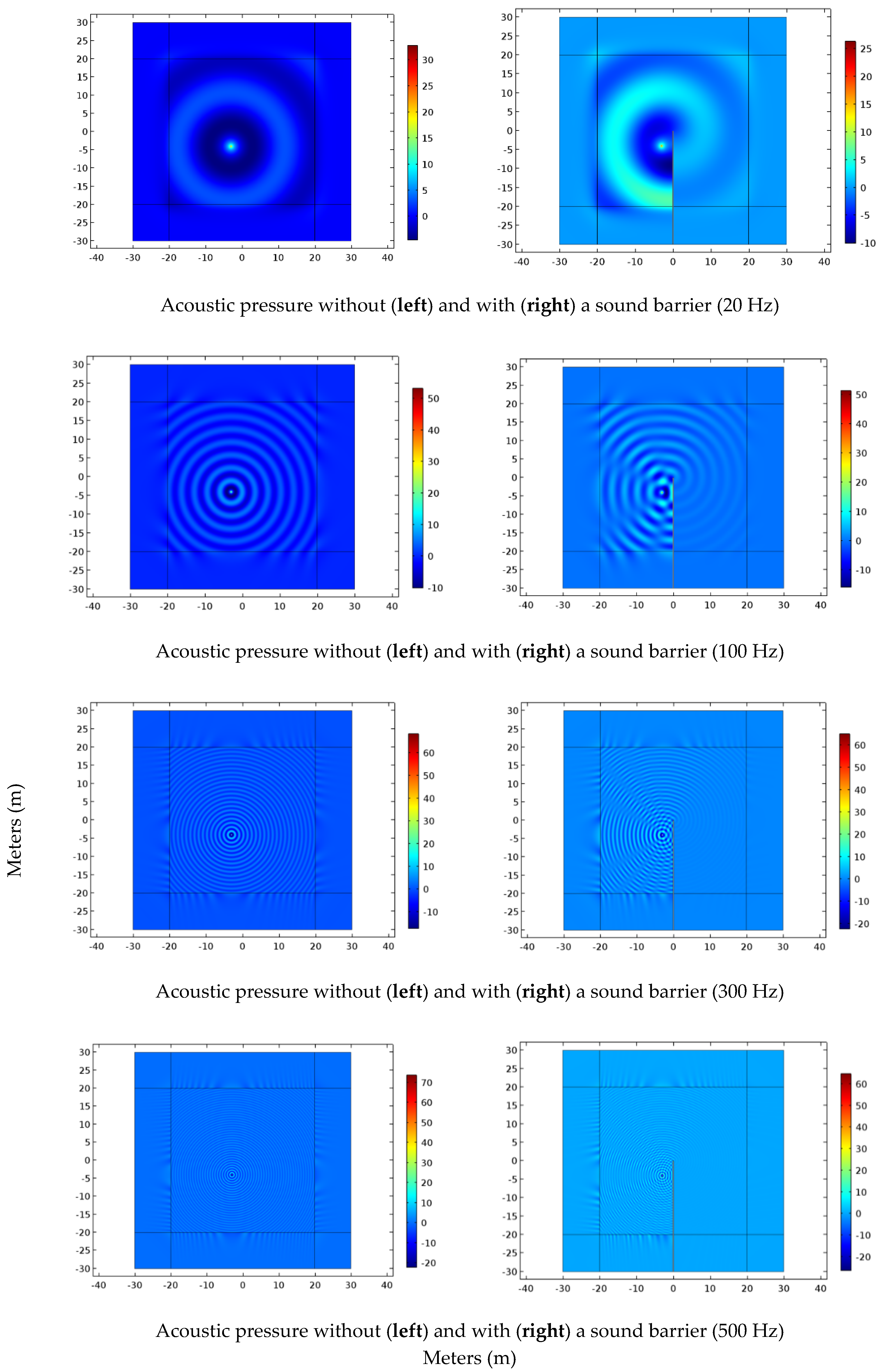
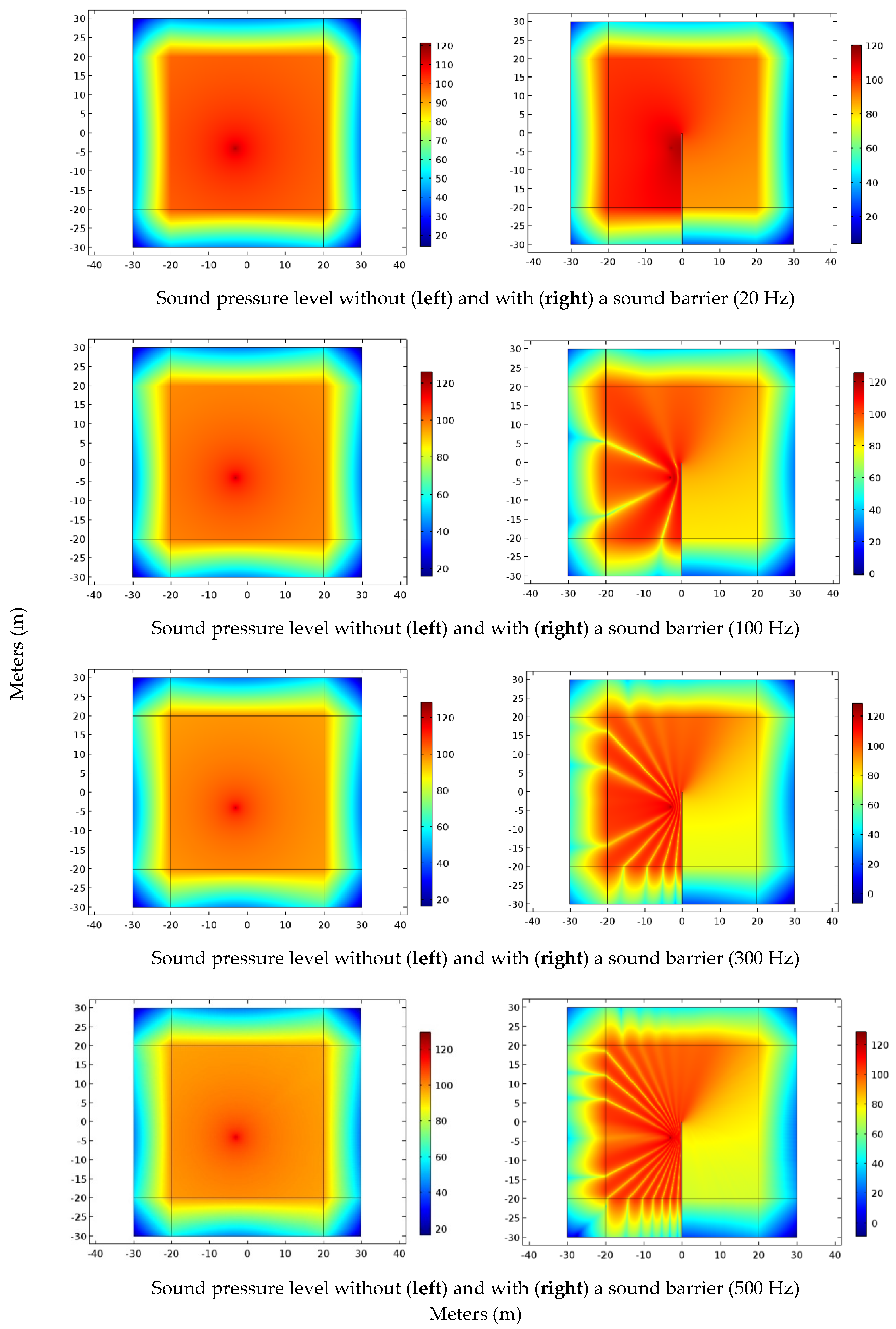
Acoustic pressures and sound pressure levels (SPL’s) were calculated via FEM. In Figure 3 and Figure 4, the acoustic pressures and SPL’s in the whole domain are presented for frequencies of 20 Hz, 100 Hz, 300 Hz, and 500 Hz respectively with and without the presence of a sound barrier. The effect of diffraction is evident in the shadow zone. Also, in the illuminated zone the interaction between the wave from the source and the reflected wave from the noise barrier can be seen. Finally, in Figure 4 in particular the effect of PML’s is apparent.
3.2. Calculation of Insertion Loss via FEM and Various Formulae
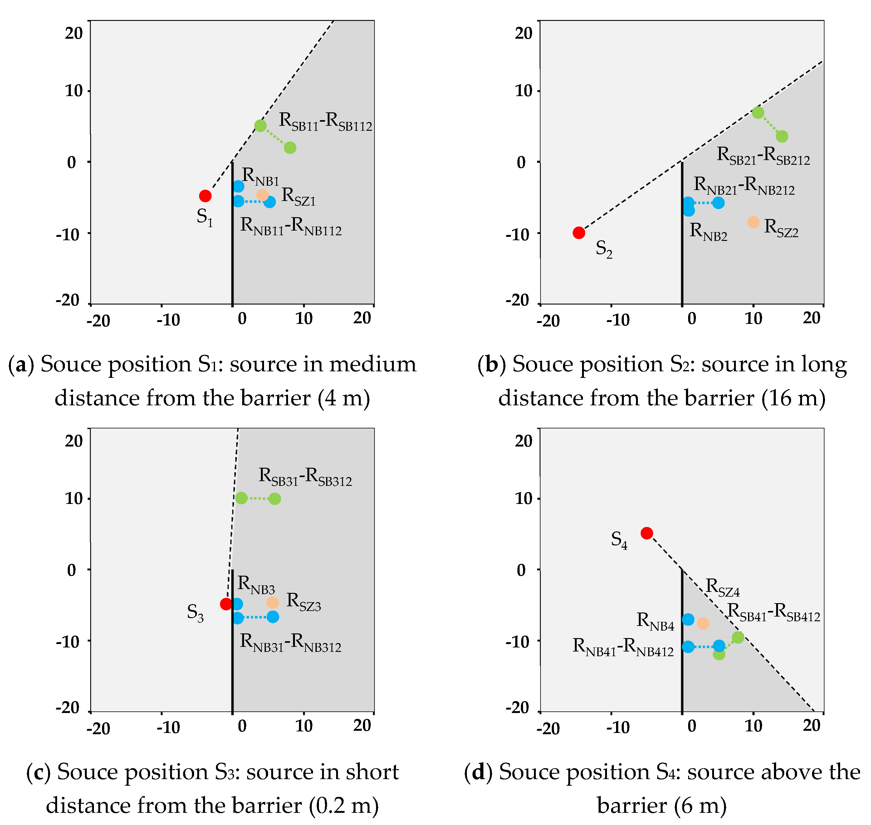
The insertion loss calculated via FEM and various formulae is presented and compared for various source and receiver positions. For the calculations, four different source positions were used:
- S1: source in medium distance from the barrier (4 m)
- S2: source in long distance from the barrier (16 m)
- S3: source in short distance from the barrier (0.2 m)
- S4: source above the barrier (6 m)
For each source position, insertion loss was investigated for the following receiver positions:
- RSZ: receiver in the shadow zone
- RSB: receiver near the shadow border
- RNB: receiver near the barrier
Source and receiver positions are presented in Figure 5, while the exact positions are given in Appendix A (Table A1).
3.2.1. Receiver in the Shadow Zone
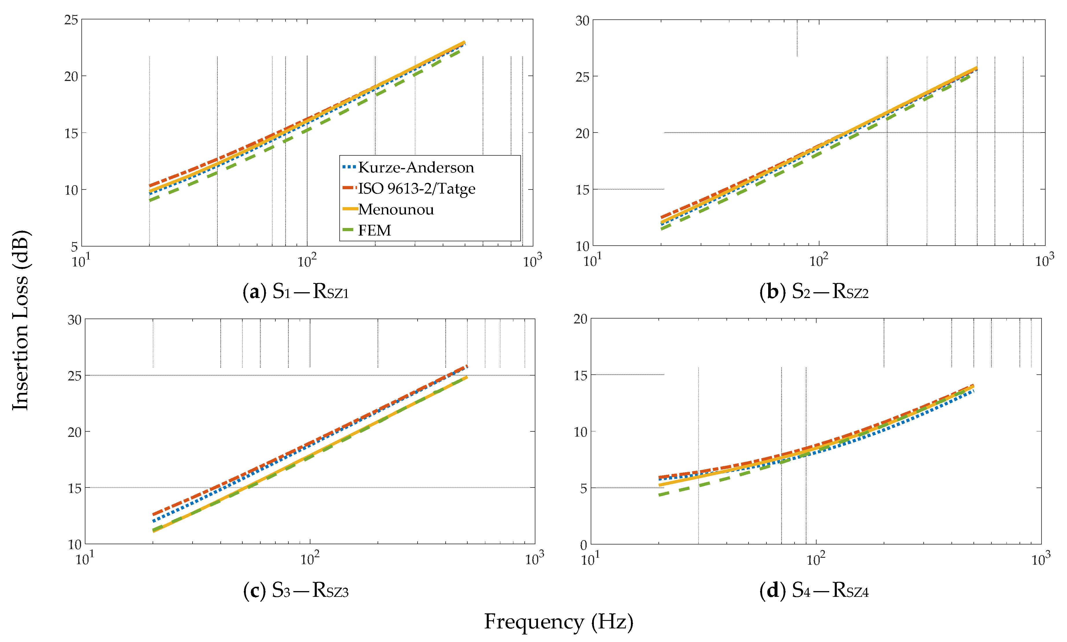
A comparison of insertion loss results between FEM and various formulae for the four source positions and receiver positions in the shadow zone is presented in Figure 6. The range of the scale on the y axis has been kept the same in each case (20 dB), so that there can be a direct comparison of the results and differences can be better discerned.
3.2.2. Receiver near Barrier (0.1 m)
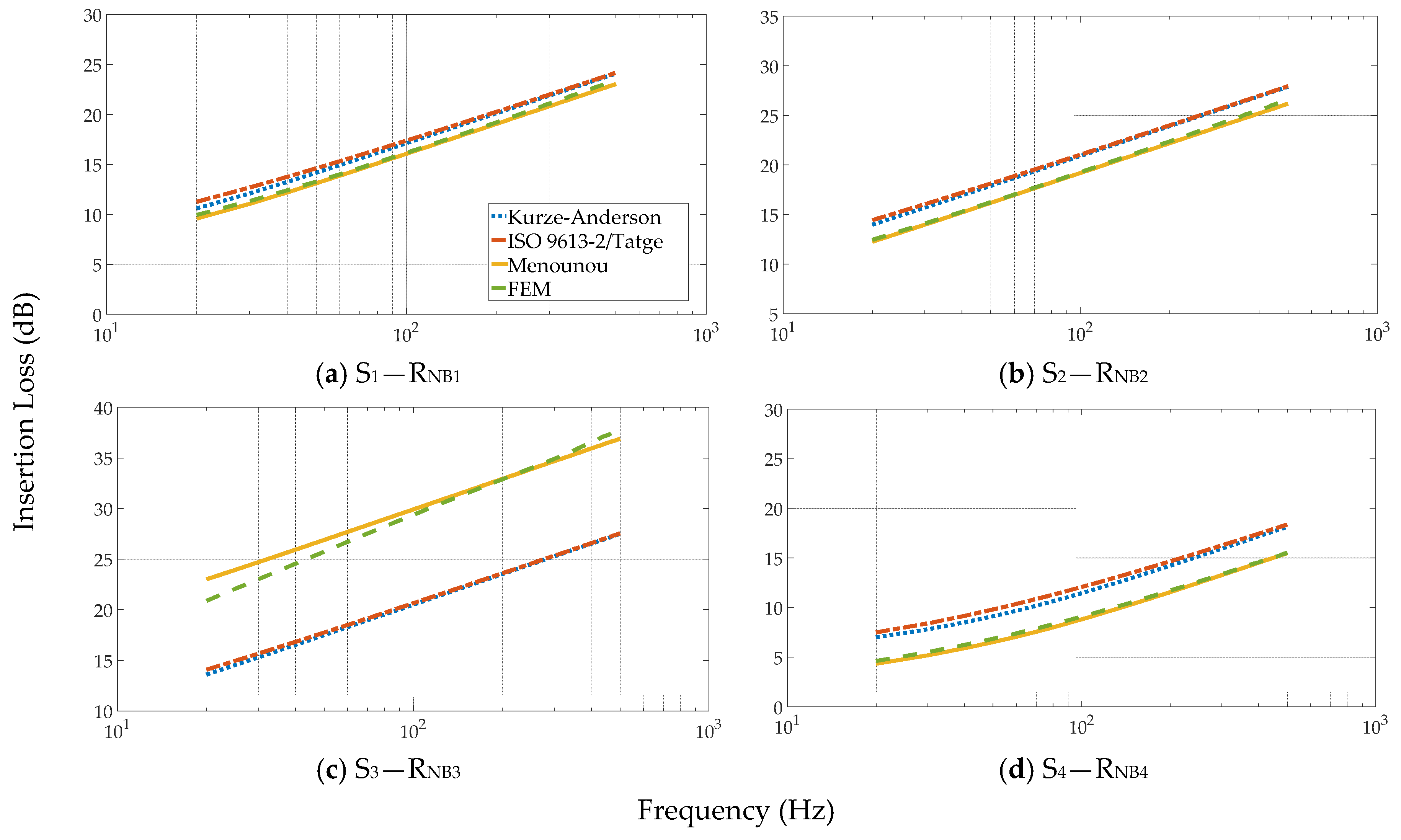
A comparison of insertion loss results between FEM and common formulae for the four source positions and receiver positions near the barrier (0.1 m) is presented in Figure 7. The range of the scale on the y axis has been kept the same in each case (30 dB), so that there can be a direct comparison of the results and differences can be better discerned.
3.2.3. Receiver in Increasing Distance from the Barrier (0.1 m–5 m)
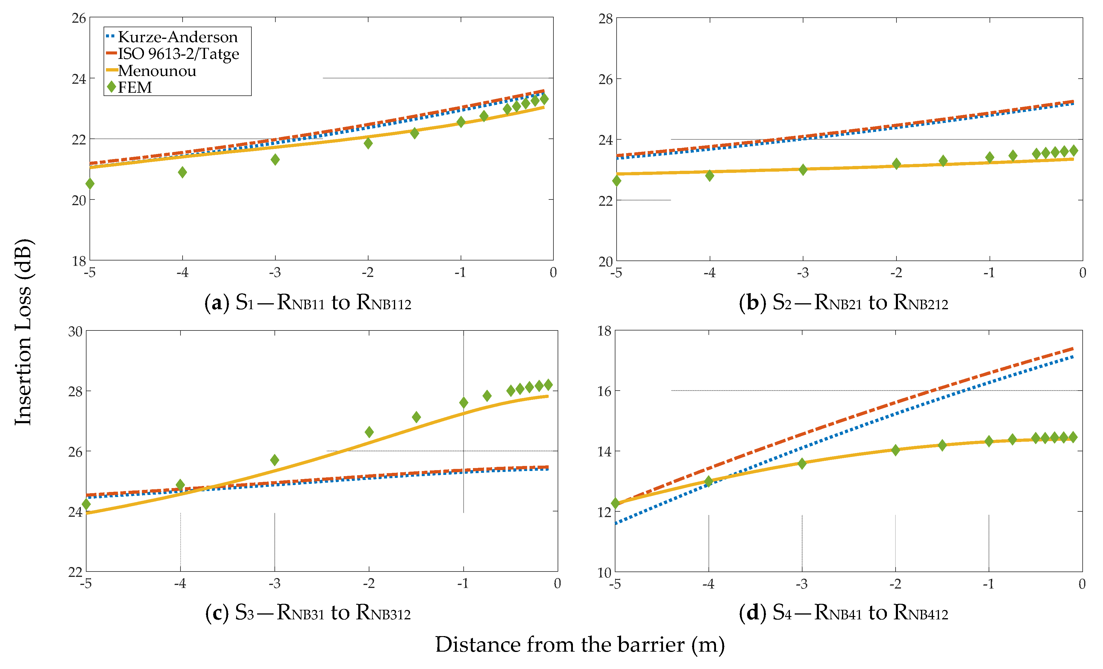
A comparison of insertion loss results between FEM and various formulae for the four source positions and receiver positions near the barrier (0.1 m–5 m) is presented in Figure 8. The range of the scale on the y axis has been kept the same in each case (8 dB), so that there can be a direct comparison of the results and differences can be better discerned.
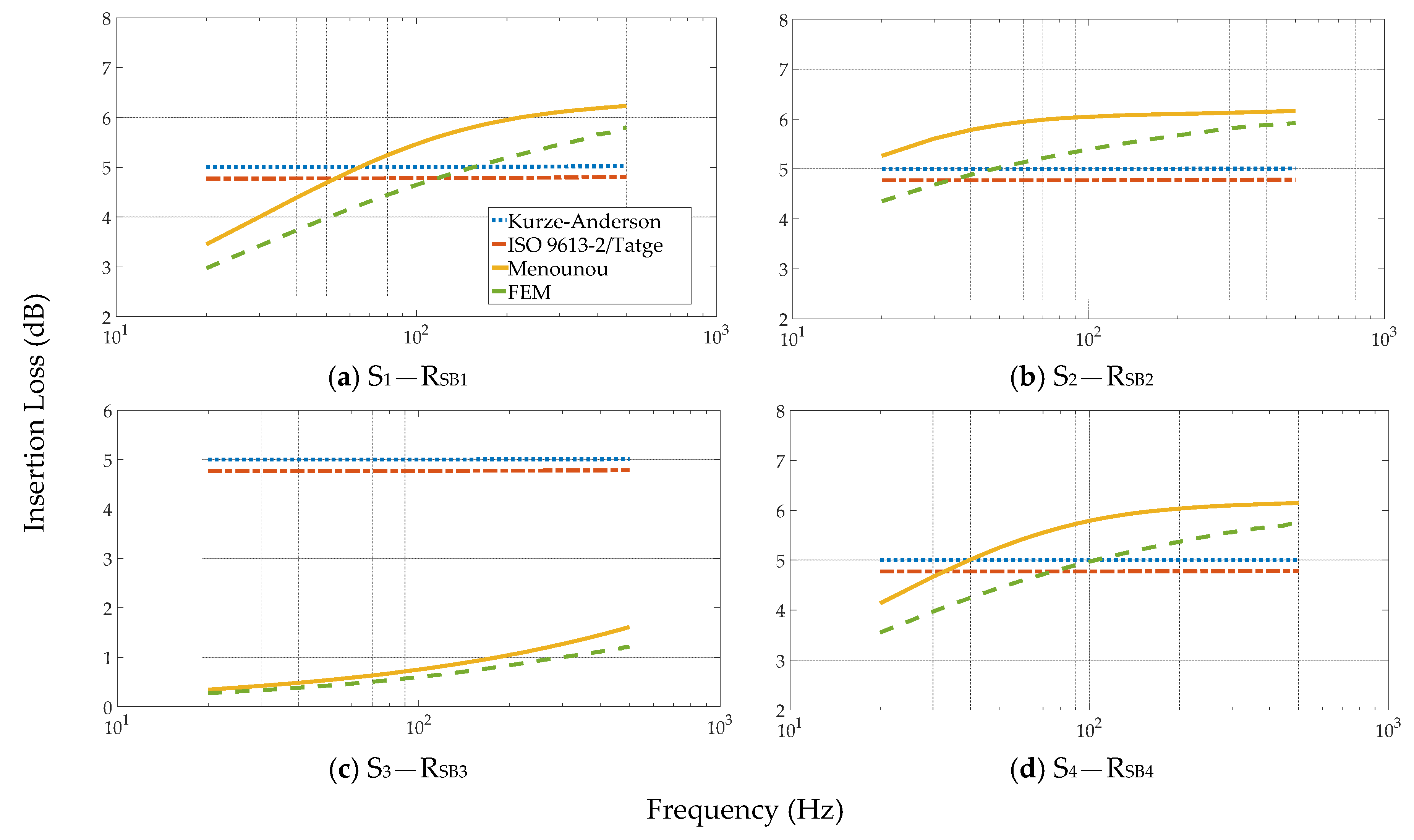
3.2.4. Receiver near the Shadow Border (0.1 m)
A comparison of insertion loss results between FEM and common formulae for the four source positions and receiver positions near the shadow border (0.1 m) is presented in Figure 9. The range of the scale on the y axis has been kept the same in each case (6 dB), so that there can be a direct comparison of the results and differences can be better discerned.
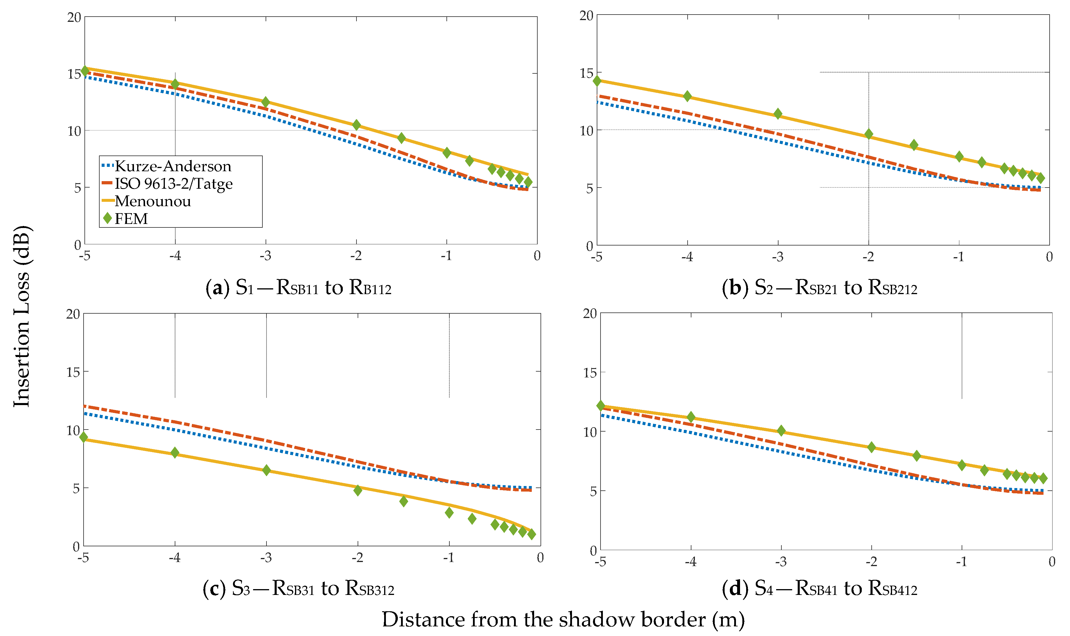
3.2.5. Receiver in Increasing Distance from the Shadow Border (0.1 m–5 m)
A comparison of insertion loss results between FEM and various formulae for the four source positions and receiver positions near the shadow border (0.1 m–5 m) is presented in Figure 10. The range of the scale on the y axis has been kept the same in each case (20 dB), so that there can be a direct comparison of the results and differences can be better discerned.
4. Discussion
The topics of this section are:
- FEM and various formulae insertion loss calculations.
- Future work and further applications of FEM for noise barriers and microscale urban acoustic modeling.
4.1. FEM and Various Formulae Insertion Loss Calculations
In the previous chapter, FEM modeling for the whole domain as well as a comparison of insertion loss calculations between FEM and various formulae for different source and receiver positions was studied.
FEM modeling in the whole domain for the acoustic pressure and the sound pressure levels is presented in Figure 3 and Figure 4. The effect of the noise barrier is evident in every area around the barrier. In particular, an interaction between the source and reflections from the noise barrier can be observed in the illuminated zone, which has a different form for each frequency. The significance of this lies in the fact that FEM allows the calculation of the sound field in the whole domain (and in the illuminated zone) where common formulae cannot apply. This is of great importance for the issue of microscale urban acoustic modeling, as the calculation of the acoustic field is important for the whole domain and is going to be discussed in the following chapter.
The comparison of insertion loss calculations between FEM and various formulae for different source and receiver positions that was presented in the results can be categorized into the following cases: receiver in the shadow zone, receiver near the barrier and receiver near the shadow border.
In the case where the receiver is in the shadow zone (Figure 6), results from FEM and all various formulae have small differences for every source position (source in medium, long, short distance and above the barrier). Especially the differences between FEM and Menounou’s formula are less than 1 dB. We must also note that in the case where the source is close to the barrier (Figure 6c), the results of FEM and Menounou’s formula are almost identical and differ from Kurze–Anderson and Tatge/ISO 9613-2 results. This is also evident in all the cases where the source is near the barrier for all the receiver positions (Figure 7c, Figure 8c, Figure 9c and Figure 10c). A possible explanation for the above result, is that since some of the formulae have emerged from semi-empirical results mainly in the shadow zone (Maekawa chart and thereafter Kurze–Anderson, Tatge/ISO 9613-2), their validity applies mainly for this area.
In the case where the receiver is near the barrier (Figure 7 and Figure 8), the results from FEM and Menounou’s formula are similar with differences less than 1 dB for almost every source position and frequency (slightly larger difference exists in the low frequency range of Figure 7c). Also, Kurze–Anderson and Tatge/ISO 9613-2 formulae follow the same pattern and present similar results. The differences between the two (Kurze–Anderson, Tatge/ISO 9613-2 and FEM, Menounou formulae) are significant especially in the case where the source is close to the barrier (about 10 dB for the whole frequency range (Figure 7c)). These results are in line with comparison of the analytical solution (McDonald solution [34]) and Kurze–Anderson formula presented in [47], where similar results were found (in the case of source and receiver close to the barrier). This is particularly important as it shows the agreement of FEM with the Menounou’s formula in the case where the receiver is near the barrier, which in turn is in agreement with the analytical solution (McDonald solution). The same trend exists at close distances (0.1 m–5 m) from the barrier (Figure 8), where FEM and Menounou’s formula seem to follow the same pattern and have similar results. Again, a possible explanation for the differences observed, is that some of the formulae have arisen from semi-empirical data mainly in the shadow zone (Maekawa chart and thereafter Kurze–Anderson, Tatge/ISO 9613-2), therefore, their validity near the noise barrier is not as good.
In the case where the receiver is near the shadow border (Figure 9 and Figure 10), once more FEM and Menounou’s formula have similar patterns and results with differences less than 1 dB. The results of Kurze–Anderson and Tatge/ISO 9613-2 formulae close to the shadow border (0.1 m) are about 5 dB in the whole frequency range for every source position. The differences between the two (Kurze–Anderson, Tatge/ISO 9613-2 and FEM, Menounou formulae) are again significant, especially in the case where the source is close to the barrier (about 5 dB for the whole frequency range (Figure 7c)). As also stated in the previous paragraph, these results are again in line with the comparison of the analytical solution (McDonald solution [34]) and Kurze–Anderson formula presented in [47], where similar results were found in the case of the receiver close to the shadow border. This result is important as it shows the agreement of FEM with Menounou’s formula in the case where the receiver is near the shadow border, which in turn is in agreement with the analytical solution (McDonald solution). The same can be observed at close distances (0.1 m–5 m) from the shadow border (Figure 10), where FEM and Menounou’s formula seem to follow the same pattern and have similar results.
In summary, there is satisfactory agreement (less than 1 dB difference in every case) of FEM and Menounou’s formula which in turn agrees with the analytical solution (McDonald solution). Especially in the cases where the receiver is near the barrier or the shadow border, FEM, and Menounou’s formula follow the same pattern and have similar results, unlike Kurze–Anderson and Tatge/ISO 9613-2, which show large deviations. In this research a large number of source and receiver positions were investigated, resulting in a wide range of applicability according to the Fresnel number. The minimum Fresnel number was 1.937 × 10⁻⁵ (Source: S3, Receiver: RSB31, Frequency: 20 Hz), while the maximum was 18.374 (Source: S2, Receiver: RSZ2, Frequency: 500 Hz). Previous research has indeed shown that the Menounou’s formula is very close in each case to the analytical solution. There are differences with the other formulae when the receiver is near the barrier and near the shadow border. The differences between the FEM/Menounou and the other formulae, have arisen probably because these formulae have been formed from semi-empirical data (e.g., Maekawa chart and thereafter Kurze–Anderson, Tatge/ISO 9613-2) in which the cases close to the barrier and near the shadow border have not been properly taken into account.
It should also be noted that FEM has advantages over Menounou’s formula for practical applications. Menounou’s formula is essentially a simple and accurate formula that provides very good results for the calculation of insertion loss in any position similar to the analytical solution for a semi-infinite noise barrier in a two-dimensional space. Therefore, it is limited to two-dimensional space and simple forms of sound barriers. The advantages of FEM are that it can be directly applied to three-dimensional space and to complex forms of noise barriers.
The results support the idea of the accuracy of FEM for the calculation of insertion loss of noise barriers. This result has further strengthened our confidence that FEM is suitable for modeling the acoustic behavior of noise barriers and its use is likely to have many applications in the future. In other words, the analytical and numerical models are very much in agreement. Their difference with the standard models is especially obvious in this case where the receiver is near the barrier or the shadow border, which in turn may have practical applications which will be discussed in the next section.
4.2. Future Work and Further Applications of FEM for Noise Barriers and Microscale Urban Acoustic Modeling
In terms of direction for future work we believe that this study provides a blueprint that can be directly utilized for modeling the acoustic behavior of noise barriers in a variety of applications. Further studies with the use of FEM could be undertaken for modeling of barriers with various shapes and configurations (e.g., in a tilt angle, galleried and cantilevered barriers etc.), for barriers that employ materials that absorb or diffuse sound, with layered materials [50], or employing atmospheric and ground absorption for a more comprehensive approach.
In terms of direction for further applications, our approach would lend itself well for use for noise barrier modeling tailored to real life problems. A common issue that has been reported regarding noise barriers is their visual impact [93], while significant positive correlations were found between aesthetic preference and environmental impact reduction, implying the importance of barrier aesthetics [94]. For barrier design ‘the best results are likely to be achieved through the co-ordinated services of qualified acousticians, civil and structural engineers, landscape architects and architects’ [17]. Due to the accuracy of FEM for modeling noise barrier, as well as its widespread use that can easily incorporate Computer-Aided Designs (CAD) (e.g., from landscape architects and architects), it could possibly applied in practice for the creation of effective and aesthetic designs that can be successfully integrated into the landscape.
A further application of FEM, utilizing similar methodology presented in this study, could possibly be for urban microscale acoustic modeling (microscale refers to small and medium-scale urban areas such as a street or a square [95]). FEM has some advantages over practices used (e.g., noise mapping software) and possibly over other wave based methods which justify further investigation for its practical application. The advantages are:
- Accuracy
- Availability
- Low cost
In real life problems, expensive noise-mapping software is used which is based on a series of algorithms specified in various standards (e.g., ISO 9613-2 [30]). A number of software packages have been developed were terms are provided for the modeling of various physical effects (e.g., screening by obstacles). A drawback associated with this approach is the neglection of the wave nature of sound, where on wave based methods (such as FEM) all wave phenomena are included in the theoretical background. Also, as presented in this study, FEM seems to provide superior results than ISO 9613-2 [30] especially in cases where the receiver or/and the source is near the barrier. This is also likely to provide better results in cases such as e.g., balconies, facades.
In terms of availability and low cost, FEM is probably the most widespread numerical method. Reliable open source FEM software exists (e.g., [96]) while also FEM is integrated in many CAD software, hence noise barrier or urban microscale acoustic modeling could possibly be incorporated in these programs, reduce application cost and spread the usage.
In general, advantages of FEM far outweigh the disadvantages which are mainly related to the computational cost. New techniques are applied in practice in order to make the computations more feasible. Utilization of Graphics Processing Unit (GPU) [97,98] has shown some remarkable results that are likely to further be improved in the future. Another way to deal with the computational issue is to use a hybrid approach in which the FEM will be applied in the low frequency range while for the higher frequencies more standard approaches will be used. FEM can also be applied in the time domain [99] for the extraction of a variety of acoustic parameters, can incorporate the effect of ground (e.g., by assigning acoustic impedance characteristics to the ground surface) [100], can model successfully the meteorological conditions [101] and since it requires discretization of the whole domain it can model an inhomogeneous atmosphere incorporating the effects of refraction [102]. A discussion of wave based methods used for microscale urban acoustic modeling can be found in [103].
5. Conclusions
We assessed the accuracy and applicability of FEM for the calculation of insertion loss of noise barriers for two dimensional acoustic radiation problems. Results obtained with FEM were compared with various formulae and especially the Menounou formula which comply well with the analytic solution. Different source and receiver positions were tested in the shadow zone, illuminated zone and in the shadow border. Particular attention was paid in the cases where the source and receiver are near the barrier and the receiver is in the shadow border, as it has been shown that results from the common Kurze–Anderson formula deviate from the analytical solution.
The findings of this study in the context of improving the urban acoustic environment support the idea that FEM can be used effectively for the accurate calculation of the insertion loss of noise barriers for various source and receiver positions and consists and excellent option for noise barrier modeling. The same scheme used in this research could be directly applied for modeling the behavior of noise barriers with various shapes and configurations and for barriers in 3D space. Our study provides practical steps that can be followed for easy implementation of FEM while strong point of our approach lies in the fact that commercial or even free software can be used. This could lead to noise barrier designs tailored to real life noise problems, thus improving the urban acoustic environment.
Although this study focuses on the implementation of FEM for noise barriers, the findings may well have a bearing on applying the method for microscale urban acoustic modeling. Although the biggest limitation lies in the computational cost, this will be less of a problem in the future while there is also the possibility of using the method in a hybrid approach for the low frequency range. This research leads to the further utilization of FEM in the context of microscale acoustic modeling, which we believe could be an important contribution as the efficiency and availability of the method can be applied in practice for the improvement of the urban environment.
Author Contributions
N.M.P. analyzed the data and wrote the manuscript; G.E.S. provided suggestions and guidance for the work, reviewed and edited the manuscript. All authors have read and agreed to the published version of the manuscript.
Funding
This research received no external funding.
Conflicts of Interest
The authors declare no conflict of interest.
Abbreviations
The following abbreviations are used in this manuscript:
| ABC | Absorbing Boundary Condition |
| BEM | Boundary Element Method |
| CAD | Computer-Aided Design |
| FDTD | Finite-Difference Time-Domain |
| FEM | Finite Element Method |
| GPU | Graphics Processing Unit |
| IL | Insertion Loss |
| PML | Perfectly Matched Layer |
| PSTD | Pseudo-Spectral Time-Domain |
| RNB | Receiver Near the Barrier |
| RSB | Receiver in the Shadow Border (near) |
| RSZ | Receiver in the Shadow Zone |
| SPL | Sound Pressure Levels |
| WHO | World Health Organization |
Appendix A

Table A1.
Source and receiver positions for calculation of insertion loss via FEM and common formulae (correspond to positions shown in Figure 5).
Table A1.
Source and receiver positions for calculation of insertion loss via FEM and common formulae (correspond to positions shown in Figure 5).
| Receiver Area | Distance d(m) | Source Positions (x,y) | |||
|---|---|---|---|---|---|
| S1(−4.00, −4.00) | S2(−16.00, −10.00) | S3(−0.20, −5.00) | S4(−6.00, 6.00) | ||
| Receiver Positions (x,y) | |||||
| Shadow zone | RSZ1(4.00, −4.00) | RSZ2(10.00, −9.00) | RSZ3(5.00, −4.00) | RSZ4(3.00, −8.00) | |
| Shadow border (0.10 m in the shadow zone) | RSB11(4.07, 3.93) | RSB21(12.05, 7.42) | RSB31(0.50, 10.00) | RSB41(8.93, −9.07) | |
| Near barrier | RNB1(0.10, −3.00) | RNB2(0.10, −8.00) | RNB3(0.10, −5.00) | RNB4(0.10, −7.00) | |
| Varying distance d from shadow border (in the shadow zone) | 0.10 | RSB11(4.07, 3.93) | RSB21(12.05, 7.42) | RSB31(0.50, 10.00) | RSB41(8.93, −9.07) |
| 0.20 | RSB12(4.14, 3.86) | RSB22(12.11, 7.33) | RSB32(0.60, 9.99) | RSB42(8.86, −9.14) | |
| 0.30 | RSB13(4.21, 3.79) | RSB23(12.16, 7.25) | RSB33(0.70, 9.99) | RSB43(8.79, −9.21) | |
| 0.40 | RSB14(4.28, 3.71) | RSB24(12.21, 7.16) | RSB34(0.80, 9.98) | RSB44(8.72, −9.28) | |
| 0.50 | RSB15(4.35, 3.65) | RSB25(12.27, 7.08) | RSB35(0.90, 9.98) | RSB45(8.65, −9.35) | |
| 0.75 | RSB16(4.53, 3.47) | RSB26(12.40, 6.86) | RSB36(1.15, 9.97) | RSB46(8.47, −9.53) | |
| 1.00 | RSB17(4.71, 3.29) | RSB27(12.53, 6.65) | RSB37(1.40, 9.96) | RSB47(8.29, −9.71) | |
| 1.50 | RSB18(5.06, 2.94) | RSB28(12.80, 6.23) | RSB38(1.90, 9.94) | RSB48(7.94, −10.06) | |
| 2.00 | RSB19(5.41, 2.59) | RSB29(13.06, 5.80) | RSB39(2.40, 9.92) | RSB49(7.59, −10.41) | |
| 3.00 | RSB110(6.12, 1.88) | RSB210(13.59, 4.96) | RSB310(3.40, 9.88) | RSB410(6.88, −11.12) | |
| 4.00 | RSB111(6.83, 1.17) | RSB211(14.12, 4.11) | RSB311(4.40, 9.84) | RSB411(6.17, −11.83) | |
| 5.00 | RSB112(7.54, 0.46) | RSB212(14.65, 3.26) | RSB312(5.40, 9.80) | RSB412(5.46, −12.54) | |
| Varying distance d near barrier (in the shadow zone) | 0.10 | RNB11(0.10, −5.00) | RNB21(0.10, −7.00) | RNB31(0.10, −7.00) | RNB41(0.10, −12.00) |
| 0.20 | RNB12(0.20, −5.00) | RNB22(0.20, −7.00) | RNB32(0.20, −7.00) | RNB42(0.20, −12.00) | |
| 0.30 | RNB13(0.30, −5.00) | RNB23(0.30, −7.00) | RNB33(0.30, −7.00) | RNB43(0.30, −12.00) | |
| 0.40 | RNB14(0.40, −5.00) | RNB24(0.40, −7.00) | RNB34(0.40, −7.00) | RNB44(0.40, −12.00) | |
| 0.50 | RNB15(0.50, −5.00) | RNB25(0.50, −7.00) | RNB35(0.50, −7.00) | RNB45(0.50, −12.00) | |
| 0.75 | RNB16(0.75, −5.00) | RNB26(0.75, −7.00) | RNB36(0.75, −7.00) | RNB46(0.75, −12.00) | |
| 1.00 | RNB17(1.00, −5.00) | RNB27(1.00, −7.00) | RNB37(1.00, −7.00) | RNB47(1.00, −12.00) | |
| 1.50 | RNB18(1.50, −5.00) | RNB28(1.50, −7.00) | RNB38(1.50, −7.00) | RNB48(1.50, −12.00) | |
| 2.00 | RNB19(2.00, −5.00) | RNB29(2.00, −7.00) | RNB39(2.00, −7.00) | RNB49(2.00, −12.00) | |
| 3.00 | RNB110(3.00, −5.00) | RNB210(3.00, −7.00) | RNB310(3.00, −7.00) | RNB410(3.00, −12.00) | |
| 4.00 | RNB111(4.00, −5.00) | RNB211(4.00, −7.00) | RNB311(4.00, −7.00) | RNB411(4.00, −12.00) | |
| 5.00 | RNB112(5.00, −5.00) | RNB212(5.00, −7.00) | RNB312(5.00, −7.00) | RNB412(5.00, −12.00) | |
| Shadow border line equations | y = x | y = 0.625x | y = 25x | y = −x | |
| Perpendicular line equations (for varying distance from the shadow border points) | y = 8 − x | y = 26.7 − 8x/5 | y = 1252/125 –x/25 | y = −18 + x | |
| Points of intersection of the above lines (x,y) | (4.00, 4.00) | (12.00, 7.50) | (0.40, 10.00) | (9.00, −9.00) | |
References
- Kang, J. Urban Sound Environment; CRC Press: Boca Raton, FL, USA, 2006. [Google Scholar]
- Berglund, B.; Lindvall, T.; Schwela, D.H. Guidel. Community Noise; Stockholm University and Karolinska Institute: Stockholm, Sweden, 1999. [Google Scholar]
- Hothersall, D.; Crombie, D.; Chandler-Wilde, S. The performance of T-profile and associated noise barriers. Appl. Acoust. 1991, 32, 269–287. [Google Scholar] [CrossRef]
- Watts, G. Acoustic performance of a multiple edge noise barrier profile at motorway sites. Appl. Acoust. 1996, 47, 47–66. [Google Scholar] [CrossRef]
- Shima, H.; Watanabe, T.; Mizuno, K.; Iida, K.; Matsumoto, K. Noise reduction of a multiple edge noise barrier. In Proceedings of the Inter-Noise 96 (Noise control: The next 25 years), Liverpool, UK, 30 July–2 August 1996; pp. 791–794. [Google Scholar]
- Fujiwara, K.; Furuta, N. SDound shielding efficiency of a barrier with a cylinder at the edge. Noise Control Eng. J. 1991, 37, 5–11. [Google Scholar] [CrossRef]
- Alfredson, R.; Du, X. Special shapes and treatments for noise barriers. In Proceedings of the Inter-Noise 95, Newport Beach, CA, USA, 10–12 July 1995; pp. 381–384. [Google Scholar]
- Iida, K.; Kondoh, Y.; Okado, Y. Research on a device for reducing noise. Transp. Res. Rec. 1984, 983, 51–54. [Google Scholar]
- Fujiwara, K.; Ohkubo, T.; Omoto, A. A note on the noise shielding efficiency of a barrier with absorbing obstacle at the edge. In INTER-NOISE and NOISE-CON Congress and Conference Proceedings; Institute of Noise Control Engineering: San Diego, CA, USA, 1995; pp. 393–396. [Google Scholar]
- Huang, X.; Zou, H.; Qiu, X. Effects of the Top Edge Impedance on Sound Barrier Diffraction. Appl. Sci. 2020, 10, 6042. [Google Scholar] [CrossRef]
- Hutchins, D.; Jones, H.; Russell, L. Model studies of barrier performance in the presence of ground surfaces. Part II—Different shapes. J. Acoust. Soc. Am. 1984, 75, 1817–1826. [Google Scholar] [CrossRef]
- Jin, B.-J.; Kim, H.-S.; Kang, H.-J.; Kim, J.-S. Sound diffraction by a partially inclined noise barrier. Appl. Acoust. 2001, 62, 1107–1121. [Google Scholar] [CrossRef]
- Wirt, L. The control of diffracted sound by means of thnadners (shaped noise barriers). Acta Acust. United Acust. 1979, 42, 73–88. [Google Scholar]
- Watts, G.R.; Hothersall, D.; Horoshenkov, K.V. Measured and predicted acoustic performance of vertically louvred noise barriers. Appl. Acoust. 2001, 62, 1287–1311. [Google Scholar] [CrossRef]
- Slutsky, S.; Bertoni, H.L. Analysis and programs for assessment of absorptive and tilted parallel barriers. Transp. Res. Rec. 1998, 1176, 13–22. [Google Scholar]
- May, D.N.; Osman, N. Highway noise barriers: New shapes. J. Sound Vib. 1980, 71, 73–101. [Google Scholar] [CrossRef]
- Kotzen, B.; English, C. Environmental Noise Barriers: A Guide to Their Acoustic and Visual Design; CRC Press: Boca Raton, FL, USA, 2014. [Google Scholar]
- Martínez-Sala, R.; Sancho, J.; Sánchez, J.V.; Gómez, V.; Llinares, J.; Meseguer, F. Sound attenuation by sculpture. Nature 1995, 378, 241. [Google Scholar] [CrossRef]
- Guo, J.; Pan, J. Increasing the insertion loss of noise barriers using an active-control system. J. Acoust. Soc. Am. 1998, 104, 3408–3416. [Google Scholar] [CrossRef]
- Wang, Y.; Zhu, X.; Zhang, T.; Bano, S.; Pan, H.; Qi, L.; Zhang, Z.; Yuan, Y. A renewable low-frequency acoustic energy harvesting noise barrier for high-speed railways using a Helmholtz resonator and a PVDF film. Appl. Energy 2018, 230, 52–61. [Google Scholar] [CrossRef]
- Voropayev, S.I.; Ovenden, N.C.; Fernando, H.J.; Donovan, P.R. Finding optimal geometries for noise barrier tops using scaled experiments. J. Acoust. Soc. Am. 2017, 141, 722–736. [Google Scholar] [CrossRef] [Green Version]
- Baulac, M.; Defrance, J.; Jean, P. Optimisation with genetic algorithm of the acoustic performance of T-shaped noise barriers with a reactive top surface. Appl. Acoust. 2008, 69, 332–342. [Google Scholar] [CrossRef]
- Zhao, W.; Chen, L.; Zheng, C.; Liu, C.; Chen, H. Design of absorbing material distribution for sound barrier using topology optimization. Struct. Multidiscip. Optim. 2017, 56, 315–329. [Google Scholar] [CrossRef]
- Kook, J.; Koo, K.; Hyun, J.; Jensen, J.S.; Wang, S. Acoustical topology optimization for Zwicker’s loudness model–Application to noise barriers. Comput. Methods Appl. Mech. Eng. 2012, 237, 130–151. [Google Scholar] [CrossRef]
- Zannin, P.H.T.; Do Nascimento, E.O.; Da Paz, E.C.; Do Valle, F. Application of artificial neural networks for noise barrier optimization. Environments 2018, 5, 135. [Google Scholar] [CrossRef] [Green Version]
- Ekici, I.; Bougdah, H. A review of research on environmental noise barriers. Build. Acoust. 2003, 10, 289–323. [Google Scholar] [CrossRef]
- Lau, S.; Tang, S. Performance of a noise barrier within an enclosed space. Appl. Acoust. 2009, 70, 50–57. [Google Scholar] [CrossRef]
- Wang, C.; Bradley, J. A mathematical model for a single screen barrier in open-plan offices. Appl. Acoust. 2002, 63, 849–866. [Google Scholar] [CrossRef] [Green Version]
- Huang, X.; Zou, H.; Qiu, X. A preliminary study on the performance of indoor active noise barriers based on 2D simulations. Build. Environ. 2015, 94, 891–899. [Google Scholar] [CrossRef] [Green Version]
- ISO 9613-2:1996. Acoustics—Attenuation of Sound during Propagation Outdoors—Part 2: General Method of Calculation; International Organization for Standardization (ISO): Geneva, Switzerland, 1996. [Google Scholar]
- Maffei, L.; Masullo, M.; Aletta, F.; Di Gabriele, M. The influence of visual characteristics of barriers on railway noise perception. Sci. Total Environ. 2013, 445, 41–47. [Google Scholar] [CrossRef] [PubMed]
- Joynt, J.L.; Kang, J. The influence of preconceptions on perceived sound reduction by environmental noise barriers. Sci. Total Environ. 2010, 408, 4368–4375. [Google Scholar] [CrossRef] [PubMed] [Green Version]
- Sommerfeld, A. Mathematische Theorie der Diffraction. Math. Ann. 1896, 47, 317–374. [Google Scholar] [CrossRef]
- Macdonald, H. A class of diffraction problems. Proc. Lond. Math. Soc. 1915, 2, 410–427. [Google Scholar] [CrossRef] [Green Version]
- Bowman, J.J.; Senior, T.B.A.; Uslenghi, P.L.E. Electromagnetic and Acoustic Scattering by Simple Shapes; Wiley-Interscience: New York, NY, USA, 1969; Volume 154, pp. 1085–1090. [Google Scholar]
- Hadden, W.J., Jr.; Pierce, A.D. Sound diffraction around screens and wedges for arbitrary point source locations. J. Acoust. Soc. Am. 1981, 69, 1266–1276. [Google Scholar] [CrossRef]
- Born, M.; Wolf, E. Principles of Optics: Electromagnetic Theory of Propagation, Interference and Diffraction of Light; Elsevier: Amsterdam, The Netherlands, 2013. [Google Scholar]
- Rubinowicz, A.; Skudrzyk, E. The Foundations of Acoustics; Springer: New York, NY, USA, 1971. [Google Scholar]
- Embleton, T.F. Line integral theory of barrier attenuation in the presence of the ground. J. Acoust. Soc. Am. 1980, 67, 42–45. [Google Scholar] [CrossRef]
- Li, K.; Wong, H. A review of commonly used analytical and empirical formulae for predicting sound diffracted by a thin screen. Appl. Acoust. 2005, 66, 45–76. [Google Scholar] [CrossRef]
- Redfearn, S. XX. Some acoustical source-observer problems. Lond. Edinb. Dublin Philos. Mag. J. Sci. 1940, 30, 223–236. [Google Scholar] [CrossRef]
- Maekawa, Z. Noise reduction by screens. Appl. Acoust. 1968, 1, 157–173. [Google Scholar] [CrossRef]
- Rathe, E. Note on two common problems of sound propagation. J. Sound Vib. 1969, 10, 472–479. [Google Scholar] [CrossRef]
- Kurze, U.; Anderson, G. Sound attenuation by barriers. Appl. Acoust. 1971, 4, 35–53. [Google Scholar] [CrossRef]
- Kurze, U.J. Noise reduction by barriers. J. Acoust. Soc. Am. 1974, 55, 504–518. [Google Scholar] [CrossRef]
- Tatge, R. Barrier-wall attenuation with a finite-sized source. J. Acoust. Soc. Am. 1973, 53, 1317–1319. [Google Scholar] [CrossRef]
- Menounou, P. A correction to Maekawa’s curve for the insertion loss behind barriers. J. Acoust. Soc. Am. 2001, 110, 1828–1838. [Google Scholar] [CrossRef]
- Kawai, T.; Fujimoto, K.; Itow, T. Noise propagation around a thin half-plane. Acta Acust. United Acust. 1977, 38, 313–323. [Google Scholar]
- Hu, Z.; Wong, R.L. Barrier insertion loss versus Fresnel number and secondary parameters. NCE 1983, 20, 31–36. [Google Scholar] [CrossRef]
- Reiter, P.; Wehr, R.; Ziegelwanger, H. Simulation and measurement of noise barrier sound-reflection properties. Appl. Acoust. 2017, 123, 133–142. [Google Scholar] [CrossRef]
- Morandi, F.; Miniaci, M.; Marzani, A.; Barbaresi, L.; Garai, M. Standardised acoustic characterisation of sonic crystals noise barriers: Sound insulation and reflection properties. Appl. Acoust. 2016, 114, 294–306. [Google Scholar] [CrossRef]
- Krynkin, A.; Umnova, O.; Chong, A.; Taherzadeh, S.; Attenborough, K. Sonic crystal noise barriers made of resonant elements. In Proceedings of the 20th International Congress on Acoustics (ICA), Sydney, Australia, 23–27 August 2010. [Google Scholar]
- Fredianelli, L.; Del Pizzo, A.; Licitra, G. Recent developments in sonic crystals as barriers for road traffic noise mitigation. Environments 2019, 6, 14. [Google Scholar] [CrossRef] [Green Version]
- Sigmund, O.; Schevenels, M.; Lazarov, B.S.; Lombaert, G. Topology optimization of two-dimensional elastic wave barriers. J. Sound Vib. 2016, 376, 95–111. [Google Scholar]
- Schevenels, M.; Lombaert, G. Topology Optimization of Elastic Wave Barriers Using a Two-and-A-Half Dimensional Finite Element Methodology. In Proceedings of the World Congress of Structural and Multidisciplinary Optimisation, Braunschweig, Germany, 5–9 June 2017; pp. 1906–1922. [Google Scholar]
- Daee, B.; El Naggar, H. 3D finite element analysis of composite noise barrier constructed of polyurethane products. Front. Struct. Civ. Eng. 2017, 11, 100–110. [Google Scholar] [CrossRef]
- Papadakis, N.M.; Stavroulakis, G.E. Estimation Of Insertion Loss of Sound Barriers via Finite Element Method. In Proceedings of the 9th GRACM International Congress on Computational Mechanics, Chania, Greece, 4–6 June 2018. [Google Scholar]
- Ishizuka, T.; Fujiwara, K. Performance of noise barriers with various edge shapes and acoustical conditions. Appl. Acoust. 2004, 65, 125–141. [Google Scholar] [CrossRef]
- Egan, C.; Chilekwa, V.; Oldham, D. An investigation of the use of the top edge treatments to enhance the performance of a noise barrier using boundary element method. In Proceedings of the 13th International Congress on Sound and Vibration, Vienna, Austria, 2–6 July 2006. [Google Scholar]
- Forssén, J.; Mauriz, L.E.; Torehammar, C.; Jean, P.; Axelsson, Ö. Performance of a Low-Height Acoustic Screen for Urban Roads: Field Measurement and Numerical Study. Acta Acust. United Acust. 2019, 105, 1026–1034. [Google Scholar] [CrossRef]
- Baulac, M.; Defrance, J.; Jean, P.; Minard, F. Efficiency of noise protections in urban areas: Predictions and scale model measurements. Acta Acust. United Acust. 2006, 92, 530–539. [Google Scholar]
- Fard, S.; Peters, H.; Marburg, S.; Kessissoglou, N. Acoustic performance of a barrier embedded with Helmholtz resonators using a quasi-periodic boundary element technique. Acta Acust. United Acust. 2017, 103, 444–450. [Google Scholar] [CrossRef]
- Oldham, D.J.; Egan, C.A. A parametric investigation of the performance of multiple edge highway noise barriers and proposals for design guidance. Appl. Acoust. 2015, 96, 139–152. [Google Scholar] [CrossRef]
- Li, Q.; Duhamel, D.; Luo, Y.; Yin, H. Analysing the acoustic performance of a nearly-enclosed noise barrier using scale model experiments and a 2.5-D BEM approach. Appl. Acoust. 2020, 158, 107079. [Google Scholar] [CrossRef]
- Koussa, F.; Defrance, J.; Jean, P.; Blanc-Benon, P. Acoustic performance of gabions noise barriers: Numerical and experimental approaches. Appl. Acoust. 2013, 74, 189–197. [Google Scholar] [CrossRef]
- Greiner, D.; Aznárez, J.J.; Maeso, O.; Winter, G. Single-and multi-objective shape design of Y-noise barriers using evolutionary computation and boundary elements. Adv. Eng. Softw. 2010, 41, 368–378. [Google Scholar] [CrossRef]
- Grubeša, S.; Jambrošić, K.; Domitrović, H. Noise barriers with varying cross-section optimized by genetic algorithms. Appl. Acoust. 2012, 73, 1129–1137. [Google Scholar] [CrossRef]
- Toledo, R.; Aznárez, J.; Maeso, O.; Greiner, D. Optimization of thin noise barrier designs using Evolutionary Algorithms and a Dual BEM Formulation. J. Sound Vib. 2015, 334, 219–238. [Google Scholar] [CrossRef] [Green Version]
- Liu, C.; Chen, L.; Zhao, W.; Chen, H. Shape optimization of sound barrier using an isogeometric fast multipole boundary element method in two dimensions. Eng. Anal. Bound. Elem. 2017, 85, 142–157. [Google Scholar] [CrossRef]
- Sakamoto, S.; Seimiya, T.; Tachibana, H. Visualization of sound reflection and diffraction using finite difference time domain method. Acoust. Sci. Technol. 2002, 23, 34–39. [Google Scholar] [CrossRef] [Green Version]
- Yokota, T.; Hirao, Y.; Yamamoto, K. Efficient calculation on outdoor sound propagation by FDTD and PE methods. Acoust. Sci. Technol. 2006, 27, 177–179. [Google Scholar] [CrossRef] [Green Version]
- Van Renterghem, T.; Botteldooren, D. Numerical simulation of the effect of trees on downwind noise barrier performance. Acta Acust. United Acust. 2003, 89, 764–778. [Google Scholar]
- Heimann, D. On the efficiency of noise barriers near sloped terrain–a numerical study. Acta Acust. United Acust. 2010, 96, 1003–1011. [Google Scholar] [CrossRef]
- Hornikx, M.; Forssén, J. Modelling of sound propagation to three-dimensional urban courtyards using the extended Fourier PSTD method. Appl. Acoust. 2011, 72, 665–676. [Google Scholar] [CrossRef]
- Van Renterghem, T.; Hornikx, M.; Smyrnova, Y.; Jean, P.; Kang, J.; Botteldooren, D.; Defrance, J. Road traffic noise reduction by vegetated low noise barriers in urban streets. In Proceedings of the 9th European Conference on Noise Control (Euronoise 2012), Prague, Czech Republic, 10–13 June 2012. [Google Scholar]
- Okuzono, T.; Otsuru, T.; Tomiku, R.; Okamoto, N. Fundamental accuracy of time domain finite element method for sound-field analysis of rooms. Appl. Acoust. 2010, 71, 940–946. [Google Scholar] [CrossRef] [Green Version]
- Papadakis, N.; Stavroulakis, G.E. Time domain finite element method for the calculation of impulse response of enclosed spaces. Room acoustics application. In Proceedings of the Mechanics of Hearing: Protein to Perception: 12th International Workshop on the Mechanics of Hearing, Cape Sounio, Greece, 23–29 June 2015; AIP Publishing LLC: Melville, NY, USA, 2015; p. 100002. [Google Scholar]
- Harari, I.; Hughes, T.J. A cost comparison of boundary element and finite element methods for problems of time-harmonic acoustics. Comput. Methods Appl. Mech. Eng. 1992, 97, 77–102. [Google Scholar] [CrossRef]
- Bolejko, R.; Dobrucki, A. FEM amd BEM computing costs for acoustical problems. Arch. Acoust. 2006, 31, 193–212. [Google Scholar]
- Möser, M. Engineering Acoustics: An Introduction to Noise Control; Springer Science & Business Media: Berlin, Germany, 2009; p. 184. [Google Scholar]
- Ihlenburg, F. Finite Element Analysis of Acoustic Scattering; Springer Science & Business Media: Berlin, Germany, 2006; Volume 132. [Google Scholar]
- Papadakis, N.M.; Stavroulakis, G.E. Effect of Mesh Size for Modeling Impulse Responses of Acoustic Spaces via Finite Element Method in the Time Domain. In Proceedings of the Euronoise 2018 Heraclion, Crete, Greece, 27–31 May 2018. [Google Scholar]
- Delaunay, B. Sur la sphere vide. Izv. Akad. Nauk SSSR Otd. Mat. Estestv. Nauk 1934, 7, 1–2. [Google Scholar]
- Sommerfeld, A. Die Greensche Funktion der Schwingungsgleichung. J. Ber. Dtsch. Math. Ver. 1912, 21, 309–353. [Google Scholar]
- Thompson, L.L. A review of finite-element methods for time-harmonic acoustics. J. Acoust. Soc. Am. 2006, 119, 1315–1330. [Google Scholar] [CrossRef] [Green Version]
- Shirron, J.J.; Babuška, I. A comparison of approximate boundary conditions and infinite element methods for exterior Helmholtz problems. Comput. Methods Appl. Mech. Eng. 1998, 164, 121–139. [Google Scholar] [CrossRef]
- Berenger, J.-P. A perfectly matched layer for the absorption of electromagnetic waves. J. Comput. Phys. 1994, 114, 185–200. [Google Scholar] [CrossRef]
- Liu, Q.-H.; Tao, J. The perfectly matched layer for acoustic waves in absorptive media. J. Acoust. Soc. Am. 1997, 102, 2072–2082. [Google Scholar] [CrossRef]
- Zampolli, M.; Malm, N.; Tesei, A. Improved perfectly matched layers for acoustic radiation and scattering problems. In Proceedings of the 2008 COMSOL Conference, Hannover, Germany, 4–6 November 2008. [Google Scholar]
- Papadakis, N.M. Application of Finite Element Method for Estimation of Acoustic Parameters. Ph.D. Thesis, Technical Univeristy of Crete, Chania, Greece, 2018. Available online: https://www.didaktorika.gr/eadd/handle/10442/42505 (accessed on 18 December 2020).
- Bermúdez, A.; Hervella-Nieto, L.; Prieto, A.; Rodrı, R. An optimal perfectly matched layer with unbounded absorbing function for time-harmonic acoustic scattering problems. J. Comput. Phys. 2007, 223, 469–488. [Google Scholar] [CrossRef]
- Marburg, S.; Nolte, B. Computational Acoustics of Noise Propagation in Fluids: Finite and Boundary Element Methods; Springer: Berlin/Heidelberg, Germany, 2008; Volume 578. [Google Scholar]
- Arenas, J.P. Potential problems with environmental sound barriers when used in mitigating surface transportation noise. Sci. Total Environ. 2008, 405, 173–179. [Google Scholar] [CrossRef] [PubMed]
- Jiang, L.; Kang, J. Combined acoustical and visual performance of noise barriers in mitigating the environmental impact of motorways. Sci. Total Environ. 2016, 543, 52–60. [Google Scholar] [CrossRef] [PubMed] [Green Version]
- Kang, J. Urban Acoustics. Appl. Acoust. 2005, 66, 121–243. [Google Scholar] [CrossRef]
- FEniCS FEM Software Documentation. Available online: https://fenicsproject.org/documentation/ (accessed on 23 June 2020).
- Chango, J.F.; Navarro, C.A.; González-Montenegro, M.A. GPU-accelerated rectangular decomposition for sound propagation modeling in 2D. In Proceedings of the 2019 38th International Conference of the Chilean Computer Science Society (SCCC), Concepcion, Chile, 4–9 November 2019; pp. 1–7. [Google Scholar]
- Mehra, R.; Raghuvanshi, N.; Savioja, L.; Lin, M.C.; Manocha, D. An efficient GPU-based time domain solver for the acoustic wave equation. Appl. Acoust. 2012, 73, 83–94. [Google Scholar] [CrossRef] [Green Version]
- Papadakis, N.; Stavroulakis, G.E. Validation of Time Domain Finite Element method via calculations of acoustic parameters in a reverberant space. In Proceedings of the 10th HSTAM International Congress on Mechanics, Chania, Greece, 25–27 May 2013. [Google Scholar]
- Attenborough, K.; Bashir, I.; Taherzadeh, S. Outdoor ground impedance models. J. Acoust. Soc. Am. 2011, 129, 2806–2819. [Google Scholar] [CrossRef] [PubMed] [Green Version]
- Yudin, M. Comparison of FDM and FEM models for a 2D gravity current in the atmosphere over a valley. Bull. Novos. Comput. Cent. 2012, 13, 95–101. [Google Scholar]
- Nomura, T.; Takagi, K.; Sato, S. Finite element simulation of sound propagation concerning meteorological conditions. Int. J. Numer. Methods Fluids 2010, 64, 1296–1318. [Google Scholar] [CrossRef]
- Hornikx, M. Ten questions concerning computational urban acoustics. Build. Environ. 2016, 106, 409–421. [Google Scholar] [CrossRef] [Green Version]
Figure 1.
Elements regarding noise barriers and insertion loss. Axes are in meters (m).

Figure 2.
Finite Element Method (FEM) model with sound barrier and Perfectly Matched Layer (Violet color). Axes are in meters (m).
Figure 2.
Finite Element Method (FEM) model with sound barrier and Perfectly Matched Layer (Violet color). Axes are in meters (m).

Figure 3.
Acoustic pressures of the domain calculated via FEM for different frequencies. Colorbar units are in Pascal (Pa). Axis units are in meters (m).
Figure 3.
Acoustic pressures of the domain calculated via FEM for different frequencies. Colorbar units are in Pascal (Pa). Axis units are in meters (m).

Figure 4.
Sound pressure levels of the domain calculated via FEM for different frequencies. Colorbar units are in SPL (dB). Axis units are in meters (m).
Figure 4.
Sound pressure levels of the domain calculated via FEM for different frequencies. Colorbar units are in SPL (dB). Axis units are in meters (m).

Figure 5.
Source and receiver positions for calculation of insertion loss via FEM and various formulae (source (S): red, receiver in the shadow zone (RSZ): orange, receiver near shadow border (RSB): green, receiver near barrier (RNB): blue). The exact positions for each source and receiver are presented in the Appendix A (Table A1).

Figure 6.
Comparison of insertion loss results between FEM and various formulae for various source and receiver positions in the shadow zone.
Figure 6.
Comparison of insertion loss results between FEM and various formulae for various source and receiver positions in the shadow zone.

Figure 7.
Comparison of calculation of insertion loss between FEM and various formulae for various source and receiver positions near the barrier inside the shadow zone.
Figure 7.
Comparison of calculation of insertion loss between FEM and various formulae for various source and receiver positions near the barrier inside the shadow zone.

Figure 8.
Comparison of calculation of insertion loss between FEM and various formulae for various source and receiver positions near the barrier inside the shadow zone (300 Hz).
Figure 8.
Comparison of calculation of insertion loss between FEM and various formulae for various source and receiver positions near the barrier inside the shadow zone (300 Hz).

Figure 9.
Comparison of calculation of insertion loss between FEM and various formulae for various source and receiver positions in the shadow border.
Figure 9.
Comparison of calculation of insertion loss between FEM and various formulae for various source and receiver positions in the shadow border.

Figure 10.
Comparison of calculation of insertion loss between FEM and various formulae for various source and receiver positions near the barrier inside the shadow zone (300 Hz).
Figure 10.
Comparison of calculation of insertion loss between FEM and various formulae for various source and receiver positions near the barrier inside the shadow zone (300 Hz).

Publisher’s Note: MDPI stays neutral with regard to jurisdictional claims in published maps and institutional affiliations. |
© 2020 by the authors. Licensee MDPI, Basel, Switzerland. This article is an open access article distributed under the terms and conditions of the Creative Commons Attribution (CC BY) license (http://creativecommons.org/licenses/by/4.0/).
Share and Cite
MDPI and ACS Style
Papadakis, N.M.; Stavroulakis, G.E. Finite Element Method for the Estimation of Insertion Loss of Noise Barriers: Comparison with Various Formulae (2D). Urban Sci. 2020, 4, 77. https://0-doi-org.brum.beds.ac.uk/10.3390/urbansci4040077
AMA Style
Papadakis NM, Stavroulakis GE. Finite Element Method for the Estimation of Insertion Loss of Noise Barriers: Comparison with Various Formulae (2D). Urban Science. 2020; 4(4):77. https://0-doi-org.brum.beds.ac.uk/10.3390/urbansci4040077
Chicago/Turabian StylePapadakis, Nikolaos M., and Georgios E. Stavroulakis. 2020. "Finite Element Method for the Estimation of Insertion Loss of Noise Barriers: Comparison with Various Formulae (2D)" Urban Science 4, no. 4: 77. https://0-doi-org.brum.beds.ac.uk/10.3390/urbansci4040077