Measuring the Differentiated Impact of New Low-Income Housing Tax Credit (LIHTC) Projects on Households’ Movements by Income Level within Urban Areas

Abstract

Social mixing is one of the key objectives of the housing policy in OECD countries. The Low-Income Housing Tax Credit (LIHTC) program, the largest affordable housing construction program in the US since 1986, has recently set creating mixed-income communities as one of the standards. As a project-based program, LIHTC developments are likely to influence residential mobility; however, little is known about its empirical effects. This study investigated whether new LIHTC projects are effective at attracting heterogeneous income groups to LIHTC neighborhoods, thereby contributing to creating mixed-income communities. Using unique individual-level household movement data combined with origin–destination neighborhood characteristics, we developed zero-inflated negative binomial (ZINB) models to analyze the LIHTC’s impact on residential mobility patterns in Franklin County, Ohio, US, from 2011 to 2015. The results suggest that the LIHTC attracts low-income households while deterring higher-income families, and therefore the program is not proved to be effective at creating mixed-income neighborhoods.

1. Introduction

In response to worsening spatial separations of rich versus poor households in terms of income, educational attainment, and jobs [1,2], deconcentrating poverty through creating mixed-income neighborhoods has been a significant focus of urban and housing policy in a number of OECD countries [3,4,5]. The strategy of creating mixed-income neighborhoods has often aimed for the integration of low-income residents into the community with greater stability, safety, and opportunity as well as neighborhood revitalization through attracting higher-income residents while fostering inclusion.

Likewise, in the US housing policy, the poverty concentration has begun to be addressed as an affordable housing policy problem since the Quality Housing and Work Responsibility Act of 1998 (QHWRA). Considerable efforts have been devoted to ensuring the availability of housing in quality neighborhoods for low-income families while attracting more affluent residents to high-poverty areas [6]. At present, deconcentrating poverty and creating mixed-income communities have become new standards to plan and evaluate housing programs (for example, housing choice vouchers and low-income housing tax credits) [7].

Among affordable housing programs, the Low-Income Housing Tax Credit (LIHTC) is the largest source of support for subsidized housing construction that provides a tax incentive for private investors to build or rehabilitate affordable housing for low-income households. While the program does not have an explicit income-mixing aim, LIHTC developments are not free from mainstream affordable housing policies. How, then, to advance the quality of neighborhoods for low-income families? LIHTC developments basically expand housing choices available to low-income families so that the quality of neighborhoods for many low-income families are often determined by the LIHTC’s location. More active interventions in location decisions (i.e., developments in low-poverty areas) have been made in accordance with the 2015 court case Texas Department of Community Affairs v Inclusive Communities Project, Inc (Dallas, Texas) [8]. Beyond the tenants themselves, LIHTC properties have spillover effects on surrounding public safety and private investment [9,10], which possibly influences residential mobility patterns, thereby changing socioeconomic compositions of neighborhoods in urban areas.

Despite a recognition that housing policy (e.g., the LIHTC) induces residential mobility [11,12], relationships between housing policy and household movements remain a “black box” for researchers and policymakers [13]. The existence of confounding factors (e.g., budget, environment, and social networks) make it difficult to establish a clear causal link between housing policy and residential mobility. More importantly, analyses have been impeded by coarse-grain data. Due to the scarcity of individual household-level residential mobility data, including data on non-recipients of housing policy, limited attention has been paid to understanding household movements as a sorting process shaping the population composition of neighborhoods in relation to housing policy. Most previous research regarding the LIHTC’s impact on neighborhoods has only focused on the resulting snapshots of population compositions of neighborhoods before and after the housing program intervention without considering the process (e.g., residential mobility) of producing the compositions [14,15]. Some exceptions using microdata relied on housing sales transaction data that only deduced neighborhood dynamics [16,17].

To fill this gap, this study aimed to understand how the LIHTC affects household movement and the residential sorting process using individual household-level residential mobility data. Specifically, we investigated whether new LIHTC projects are effective in drawing middle- and high-income households into LIHTC neighborhoods so that they potentially contribute to alleviating the poverty concentration and developing mixed-income communities. Taking Franklin County, Ohio, US, as a case, gravity models with a zero-inflated binomial specification were employed to examine the impact of the LIHTC on residential mobility between 2011 and 2015. Using a gravity model, our analysis attempts to measure the impacts of the housing policy within the comprehensive migration pattern (i.e., including non-zero flows) in consideration of neighborhoods’ characteristics.

2. Literature Review

The LIHTC has been the largest federal housing program, providing funding for almost three million units of affordable rental housing in the US since its inception in 1986 [18]. The program’s primary goal is to increase the supply of affordable housing for lower-income households [19,20]. The Omnibus Reconciliation Act of 1989 encourages the private sector to provide LIHTCs in hard-to-service neighborhoods by providing more tax credits, for example, in areas with qualified census tracts (QCTs) that have more than half of households earning less than 60% of area median income (AMI) and difficult development areas (DDAs) that have more expensive development costs than household incomes [21]. Since 2000, state finance housing agencies began giving incentives to LIHTC projects in QCTs, which have been criticized for concentrating LIHTC projects in high-poverty and majority-minority neighborhoods [21,22].

Beyond the welfare impact on tenants living in LIHTC units, scholars have hoped for spillover effects, revitalizing communities and creating mixed-income neighborhoods by attracting diverse residents [7]. The LIHTC, as a place-based program, induces changes in neighborhoods, which in turn might attract some new residents while discouraging others [9,23,24]. Although little empirical evidence exists on how the LIHTC affects residential mobility patterns, studies regarding the spillover effects of LIHTC projects on surrounding neighborhoods provide initial clues about how the LIHTC may result in the inflow and outflow of residents across income levels. The empirical literature on the LIHTC thus far has found mixed results about its effect on neighborhood changes in housing values, public safety, and composition of residents.

First, the LIHTC has heterogeneous effects on surrounding housing prices depending on where LIHTC projects are located. Positive effects on housing values were found when LIHTC developments enhanced a neighborhood’s amenities by replacing deteriorated buildings and vacant lands in lower-income areas [9,10,25,26]. Koschinsky reported that the positive effects might be driven by housing sales in poverty pockets within more affluent areas [27], and Woo et al. argued that the LIHTC exerted a stimulating effect in Cleveland, which had a stagnant housing market [24]. Conversely, in affluent neighborhoods, LIHTC developments can be conceived as undesirable due to the influx of lower-income households and their negative tax-to-service rate [24]. Studies found a negative impact on sales prices of houses near LIHTC projects in Charlotte [17] and Philadelphia [28], both of which have rapidly appreciating housing markets. Diamond and McQuade also found that LIHTC developments caused house price declines of 2.5% in neighborhoods with higher median incomes and a majority white population [16].

Second, prior studies examining the impact of the LIHTC on public safety produced conflicting results. LIHTC developments may contribute to decreasing crime by removing blight and adding more eyes on the street [19,26], as they attract a greater police presence and have security systems in place [29]. Freedman and Owens found that LIHTCs bring significant reductions in violent crime to most impoverished neighborhoods at the county level [29]. Diamond and McQuade found that LIHTC projects contribute to lower crime rates in low-income neighborhoods and do not appear to increase crime in high-income areas [16]. However, a large body of research examining relationships between crime and public housing suggests that the concentration of the disadvantages of large developments likely contributes to small crime increases in surrounding neighborhoods [30].

Third, while reports contend that LIHTC developments trigger the flow of residents in and out of neighborhoods, altering the residential composition, the directions remain uncertain. Studies that found positive effects argued that the LIHTC makes a distressed minority neighborhood more attractive to diverse households by removing blight, repopulating a community, and/or attracting other investments and improvements [26,31]. Diamond and McQuade found that homebuyers purchasing properties near newly completed LIHTC units have slightly higher incomes and non-black shares than the local average in lower-income areas [16]. Similarly, examining changes in the racial composition of tracts in which LIHTC developments were located, Horn and O’Regan found that neighborhoods with high minority concentrations experienced declines in the minority share over time [15]. In lower-poverty neighborhoods, studies suggested that LIHTC developments contribute to “white flight” based on fear and concern of the influx of “undesirables” into affluent neighborhoods [24,32]. Woo et al. found that LIHTC developments increased housing turnover rates even more in high-income neighborhoods [24], and Diamond and McQuade found that higher-income households in affluent neighborhoods were willing to pay more to live further away from LIHTC units [16]. Conversely, Freedman and McGavock found little evidence that higher-income households leave neighborhoods in response to LIHTC developments [23].

Findings generally indicate that LIHTC projects have contributed to revitalizing distressed neighborhoods by increasing housing prices, lowering crime rates, and attracting diverse residents. However, it remains uncertain whether improvements have been in accordance with the outflow of low-income residents from revitalized neighborhoods, which may be part of the gentrification process. Furthermore, given that a growing number of LIHTC projects are located in suburban low-poverty tracts [33,34], the impact on affluent neighborhoods, whether LIHTC projects trigger outflow of higher-income residents and/or inflow of lower-income residents, needs to be examined. The study fills the knowledge gap by analyzing the effects of LIHTC on residential mobility across income levels using individual household-level movement data.

3. Materials and Methods

3.1. Study Area

This study analyzed the impact of LIHTCs on residential mobility in Franklin County, Ohio, US, during a 5-year LIHTC deployment period (2011–2015). Franklin County, Ohio’s state capital, is among the fastest-growing counties in the US and had a population of over 1.3 million as of 2019. Franklin County has experienced persistent suburbanization and economic and racial segregation (west vs east and north vs south divides) throughout the last several decades, following a national trend [2,35]. Northwestern parts of the county have consistently lower rates of unemployment, with white and middle-income neighborhoods, while southern Franklin County, especially the southeast, has a concentration of African Americans and low-income families [36]. A recent study also reported a deepening gap and increasing polarization in housing prices and neighborhood values around the Franklin County region based on housing transactions data [37]. Accordingly, the provision of affordable housing has become an increasingly serious concern in Franklin County [38]. The Ohio Housing Finance Agency (OHFA) has promoted mixed-income development since 1997 and recently reconfigured the Qualified Allocation Plans to incentivize affordable housing development in economically flourishing neighborhoods [39].

Since 1987, a total of 249 LIHTC projects have been supplied in Franklin County. A total of 32 projects placed in service from 2011 to 2015 provided about 1,902 housing units, of which approximately 98.9% housed low-income households. Approximately 70% of these projects were newly constructed, whereas the average during the same period in the state of Ohio was 53%. More than half of these projects were located in QCTs (56%), which was a higher share than the state average (42%). None of the projects were provided in DDAs. There were two projects specifically targeted for the homeless. A total of 25 census tracts that introduced LIHTC projects between 2011 and 2015 were in distressed conditions relative to the state. These tracts had a higher poverty rate (27.6%) than the county average (16.5%) as of 2011. However, 8 out of 25 census tracts were below the average poverty rate.

3.2. Data

3.2.1. Longitudinal Residential Mobility Data

We used data from the Data Axle Historical Consumer Database (previously InfoGroup) to construct a longitudinal database on residential location changes for a cross-section of the population between 2011 and 2015. The Data Axle data are of high temporal resolution (i.e., updated monthly) and comprise a unique micro dataset of 155 million households in the US [40]. The data come with households’ addresses at a census tract level and socioeconomic statuses such as annual income, household head age, marriage status, and ownership status. A unique identification number (household ID) assigned to each household enables linking records over time so that we can capture household-level residential mobility patterns from one census tract to another [13]. Researchers are increasingly using the data to examine residential mobility at a fine-grain scale in relation to neighborhood change [13], neighborhood type [41], and location preferences [42].

To construct matrices of the household movement at the census tract level, we first merged residential location data in Franklin County for 2011 and 2015 by household ID, retrieving the data for 339,461 households (74.7% of the total number of households in the county [43]). The under-coverage rate of 25.3% in the study area is higher than that of the national average (15.4%) identified by Kennel and Li [44]. A Pearson correlation coefficient of the number of households between the Data Axel dataset and 2011–2015 American Community Survey (ACS) five-year estimates is 0.97 (p < 0.001), which reveals that the dataset is less likely to suffer from selection bias. We then identified a total of 41,030 households (12.1% of the matched households) that changed their addresses from one census tract to another. We limited the scope of our analysis to intra-county residential mobility patterns because different factors influence households’ movement decisions depending on the scales of the move (e.g., inter-county vs. intra-county) [13,45,46]. In fact, the literature suggests that a large portion of residential mobility occurs within a county [47]. According to the 2007–2011 ACS 5-year estimates, among 289,277 households that moved in the past year in Franklin County, 186,773 (64.6%) moved within the county, 83,432 (28.8%) moved from a different county in Ohio, and 19,072 (6.6%) moved from a different state. The 5-year period (2011–2015) was selected to reduce the possibility that movement flows were compounded by changing neighborhood characteristics that resulted from the moves [48], while securing enough household movement numbers to identify intra-county residential mobility patterns.

Constructing our dependent variable (the number of moves between neighborhoods by income) necessitated categorizing households into different income groups. We defined households earning twice the county median household income as high-income groups and households below two-thirds of the median income as low-income groups. The rest were defined as middle-income groups. While there are currently several legislated income limit standards (e.g., HUD defines under 50% of the median family income as very low income and under 80% as a low-income family), we followed the scheme that has been adopted in prior studies [46,49]. We then pooled each group’s moves into an origin–destination matrix that described the total number of moves from one census tract to another, between 2011 and 2015 within Franklin County, even if these were zero. We excluded neighborhoods with fewer than 10 residents or 0 median housing value. In the origin–destination matrix, 75,900 unique origin–destination pairings connected 276 census tracts in Franklin County.

3.2.2. Neighborhood Composition Data

We used the total housing units, share of owner-occupied, share of white population, share of families with children, and housing values from 2007–2011 ACS 5-year estimates [50] to describe the socioeconomic composition of neighborhoods at a census tract level. Following the assumption that a household decided to move considering current or previous neighborhood status, 2007–2011 ACS data were employed to describe neighborhood characteristics before the move occurred (we assessed the household movements between 2011 and 2015). We retrieved the number of housing unit data from both 2007–2011 and 2011–2015 ACS to calculate the growth rates of the number of housing stocks [49]. We confirmed that the census tract boundaries of the county had been relatively persistent during the 5 years, without significant changes (i.e., split, merge). We also obtained the Urbanization Perceptions Small Area Index (UPSAI) as a proxy for neighborhood classification into urban, suburban, and rural from the US Department of Housing and Urban Development (HUD). The data were based on the 2017 American Housing Survey asking respondents to describe their neighborhood as urban, suburban, or rural at a census tract level adjusted using the machine learning technique [51]. The census tract level data were then joined to the origin–destination matrix for a gravity model.

3.2.3. LIHTC Data

We used data from the HUD on LIHTC projects completed in Franklin County during 1987–2019. The data provided information on each project, including addresses, total low-income units, construction type, and placed-in-service years. Following the approach adopted by Nilsson and Delmelle [46], we examined the impact of new LIHTC projects completed within ±2 years of the research period, namely from 2009 to 2017, on households’ decisions to move. We assume that the impact of new LIHTC projects on households’ decisions to move was limited within ±2 years encompassing the announcement of development to spur investments. To control the potential impact of the existing LIHTC units, the number of units supplied before the 2-year time window (LIHTCs constructed before 2009) was calculated and utilized. We geocoded the locations of LIHTC projects and then attributed them to the corresponding census tract.

3.3. Model and Operationalization of Variables

We identified the impact of new LIHTC projects on relocation decisions across census tracts by household income levels using gravity models with a zero-inflated negative binomial (ZINB) specification. Gravity models, analogous models of Isaac Newton’s theory of universal gravitation, are popular for analyzing residential mobility patterns at various spatial scales [52,53]. The models has been criticized for their endogeneity and the absence of theoretical foundations and dynamics [54], and alternative approaches such as network modeling [55] and agent-based models [56] have been proposed. Other econometric models have been proved to have their own advantages. For example, multinomial discrete choice models allow for explaining location choice from individual characteristics of movers. Difference-in-difference models can assess the policy impact caused by the implementation of new facilities. However, in our view, gravity models are better suited to capture detailed spatial structures that influence residential mobility. By incorporating all possible origin–destination combinations (even zero-flow observations), gravity models can address spatial effects which neighborhoods can have on leaving the current location and choosing a new one, without difficulties in sampling and defining the reference category in other models.

The simplest version of gravity models consists of two factors, mass and distance, based on the assumption that migration flows are driven by attractive forces between neighborhoods (often reflected by population or GDP) and impeded by the costs (or frictions) of moving from one neighborhood to another. We adopted the number of housing units in origin and destination as mass variables. While the distance generally refers to the physical distance calculated as the Euclidean distance between centroids of neighborhoods, similar to the approach adopted by Bakens et al. [48], we extended the concept to encompass socioeconomic distances between neighborhoods. We measured socioeconomic distances by calculating the difference in a socioeconomic attribute between the neighborhoods of origin and destination as follows:

$$D_{ij}=S_j-S_i$$

(1)

where $S$ is the household share of each socioeconomic characteristic in origin $i$ and destination $j$. The socioeconomic distances were calculated for: the share of owner-occupied; share of white population; share of families with children; housing values; share of new LIHTC units for low-income households among the total housing units. This method of conceptualizing—measuring differences between neighborhoods—measures to what extent socioeconomic differences act as barriers to migration [48,57,58] on the one hand, and allows our models to examine to what extent people value the socioeconomic characteristics of the destination relative to the origin, on the other hand [59]. A positive coefficient of the socioeconomic distance variables corresponds to a preference tendency toward a neighborhood with a higher attribute value. For example, if the coefficient of “the distance of white population” was positive, we said that households preferred to move to neighborhoods with a higher share of white population compared to neighborhoods they had lived in. Conversely, a negative coefficient suggested a preference for living in neighborhoods with a smaller white population, which revealed that the racial difference served as a barrier to move. Therefore, it was assumed that differences in LIHTC units may act either as preferred amenities or additional barriers (disamenities) to migration. We considered the varying effects by the project size [17] by calculating the proportion of LIHTC units among the total housing units in a neighborhood. We also included quadratic terms ($D_{ij}^2$) for the socioeconomic distance variables to check for potential non-linear relationships.

In addition to mass and distance variables, the housing stock growth rate between 2011 and 2015 in the destination neighborhood was included as a control variable. As LIHTC control variables, (1) the share of LIHTC units completed before the movement decision was made (1988–2009) among the total housing units and (2) the dummy variable of new LIHTC projects designed to target homeless households in both origin and destination were included. These two variables controlled for the impact of the existing LIHTC units as well as a potential tendency to avoid homeless-targeted projects compared to other LIHTC projects. Due to the scarce information about the impact of homeless-targeted units, we operationalized it as a dummy variable to be 1 if a unit exists. Controlling for unobserved neighborhood characteristics, we included the UPSAI indicating to what extent an origin or a destination neighborhood was considered urban or suburban by its residents. We included fixed effects to account for income group-specific unobserved characteristics that impact mobility.

Table 1. Descriptive statistics of model variables.

Variables	Description	Min.	Max.	Mean.	Std. Dev.
Dependent variables
High income	The number of moves of households between 2011 and 2015 whose annual income exceeded twice the county median household income	0	42	0.09	0.63
Middle income	The number of moves of households between 2011 and 2015 whose annual income was between two-thirds and twice the county median household income	0	43	0.21	0.89
Low income	The number of moves of households between 2011 and 2015 whose annual income was lower than two-thirds of the county median household income	0	39	0.23	0.8
Independent variables
Number of housing units	Total number of households in the origin. Logarithmized in the models.	572	7561	1884	883.5
Physical distance	Absolute distance between the centers of origin and destination. Logarithmized in the models.	0.48	44.0	14.1	7.1
Dij Share owner occupied	Difference in shares of owner-occupied housing units between destination and origin	−0.98	0.98	0	0.33
Share white population	Difference in shares of white population between destination and origin	−0.98	0.98	0	0.37
Share families with children	Difference in shares of families with children between destination and origin	−0.69	0.69	0	0.16
Housing value	Difference in housing value between destination and origin. Logarithmized in the models.	−3.99	3.99	0	0.69
Share LIHTC units (±2 years)	Difference in shares of LIHTC units placed between 2009 and 2017 among the total housing units between destination and origin	−0.23	0.23	0	0.03
Control variables
Existing LIHTC units (−2 years)	Share of LIHTC units placed before 2009 among the total housing units in origin and destination	0	1	0.03	0.09
Homeless-targeted LIHTC (±2 years)	Dummy variable of LIHTC project that specifically targets homeless households placed between 2009 and 2017 in origin and destination (1 if yes)	0	1	0.01	0.12
Housing stock growthj	growth rate of the number of housing stocks between 2011 and 2015 in destination	−0.2	0.41	0.02	0.07
Neighborhood fixed effects	Urban: share of responses that they live in urban areas	0	1	0.38	0.34
	Suburban: share of responses that they live in suburban areas	0	0.83	0.02	0.08

Source: Data Axle (2021), US Census Bureau (2011; 2015), and HUD (2021). Quadratic terms (D_ij²) for all socioeconomic distance variables (D_ij) were included.

shows descriptive statistics for the variables in our models. The mean distance variable values were all zero because differences in all pairs of neighborhoods generated perfectly symmetrical distributions of the variables.

To estimate the count data (the number of moves between census tracts) in our study, we used zero-inflated negative binomial (ZINB) models. As a modified Poisson model, the ZINB effectively accounts for problems in modeling count data with overdispersion (the variance is greater than the mean) and excessive zeros [60,61]. The ZINB specification considers two groups within the population: (1) a group with strictly zero counts and (2) a group with a non-zero probability of counts greater than zero. These two groups are modeled using a logit regression and negative binomial regression, respectively, within the ZINB framework [62]. Coefficients in the logit part and corresponding coefficients in the negative binomial part generally have opposite signs due to the logit part predicting the chance of belonging to the “strictly zero group.” The probabilities of a zero count and a positive count can be specified as Equations (2) and (3), respectively, as follows [61]:

$$\mathrm{Pr}\left({\mathrm{M}}_{\mathrm{ij}}=0\right)={\mathsf{\pi }}_{\mathrm{ij}}+\left(1-{\mathsf{\pi }}_{\mathrm{ij}}\right){\left(\frac{{\mathsf{\alpha }}^{-1}}{{\mathsf{\alpha }}^{-1}+{\mathsf{\mu }}_{\mathrm{ij}}}\right)}^{{\mathsf{\alpha }}^{-1}}$$

(2)

$$\mathrm{Pr}\left({\mathrm{M}}_{\mathrm{ij}}\right)=\left(1-{\mathsf{\pi }}_{\mathrm{ij}}\right)\frac{\mathsf{\Gamma }\left({\mathrm{M}}_{\mathrm{ij}}+{\mathsf{\alpha }}^{-1}\right)}{{\mathrm{M}}_{\mathrm{ij}}!\mathsf{\Gamma }\left({\mathsf{\alpha }}^{-1}\right)}{\left(\frac{{\mathsf{\alpha }}^{-1}}{{\mathsf{\alpha }}^{-1}+{\mathsf{\mu }}_{\mathrm{ij}}}\right)}^{{\mathsf{\alpha }}^{-1}}{\left(\frac{{\mathsf{\mu }}_{\mathrm{ij}}}{{\mathsf{\alpha }}^{-1}+{\mathsf{\mu }}_{\mathrm{ij}}}\right)}^{{\mathrm{M}}_{\mathrm{ij}}}$$

(3)

where ${\mathsf{\pi }}_{\mathrm{ij}}$ is the logistic link function that the probability of a move being in the always zero group and the conditional mean (${\mathsf{\mu }}_{\mathrm{ij}}$) that is linked to an exponential function of a set of explanatory variables is defined as:

$${\mathsf{\mu }}_{\mathrm{ij}}=\exp ({\mathrm{a}}_0+{\mathrm{a}}_1{\mathrm{lnP}}_{\mathrm{i}}+{\mathrm{a}}_2{\mathrm{lnP}}_{\mathrm{j}}+{{\displaystyle \sum }}_{\mathrm{k}}{\mathrm{a}}_{3\mathrm{k}}{\mathrm{lnX}}_{\mathrm{ik}}+{{\displaystyle \sum }}_{\mathrm{k}}{\mathrm{a}}_{4\mathrm{k}}{\mathrm{lnX}}_{\mathrm{jk}}+{\mathrm{blnd}}_{\mathrm{ij}})$$

(4)

In the analysis, we used (1) the overdispersion test to see whether the negative binomial model was preferable to the Poisson model and (2) the boundary likelihood ratio test to examine whether the ZINB was superior to the negative binomial model [63,64]. We used the log-likelihood and Akaike information criterion (AIC) to evaluate our models’ fit.

Based on matrices separately defined for each income group, we estimated the model for all of the groups together to compare the results across the different income groups. Thus, the total number of observations was 227,700 (75,900 × 3). The LIHTC-related variables interacted with an income group dummy, with an assumption that the impact of the other variables was homogeneous across the groups. As robustness checks, we ran models separately for each group to examine if the different impact of all of the variables by income group changed the direction of the results. We also applied alternative definitions of income levels and different definitions of new LIHTC units using varying time windows to check the robustness of the results. Variance inflation factors (VIF) in all of the models were lower than 2, except for a few quadratic terms, which confirmed no multicollinearity problem in our models. R 3.5.0. was used for the ZINB models and visualization.

4. Results

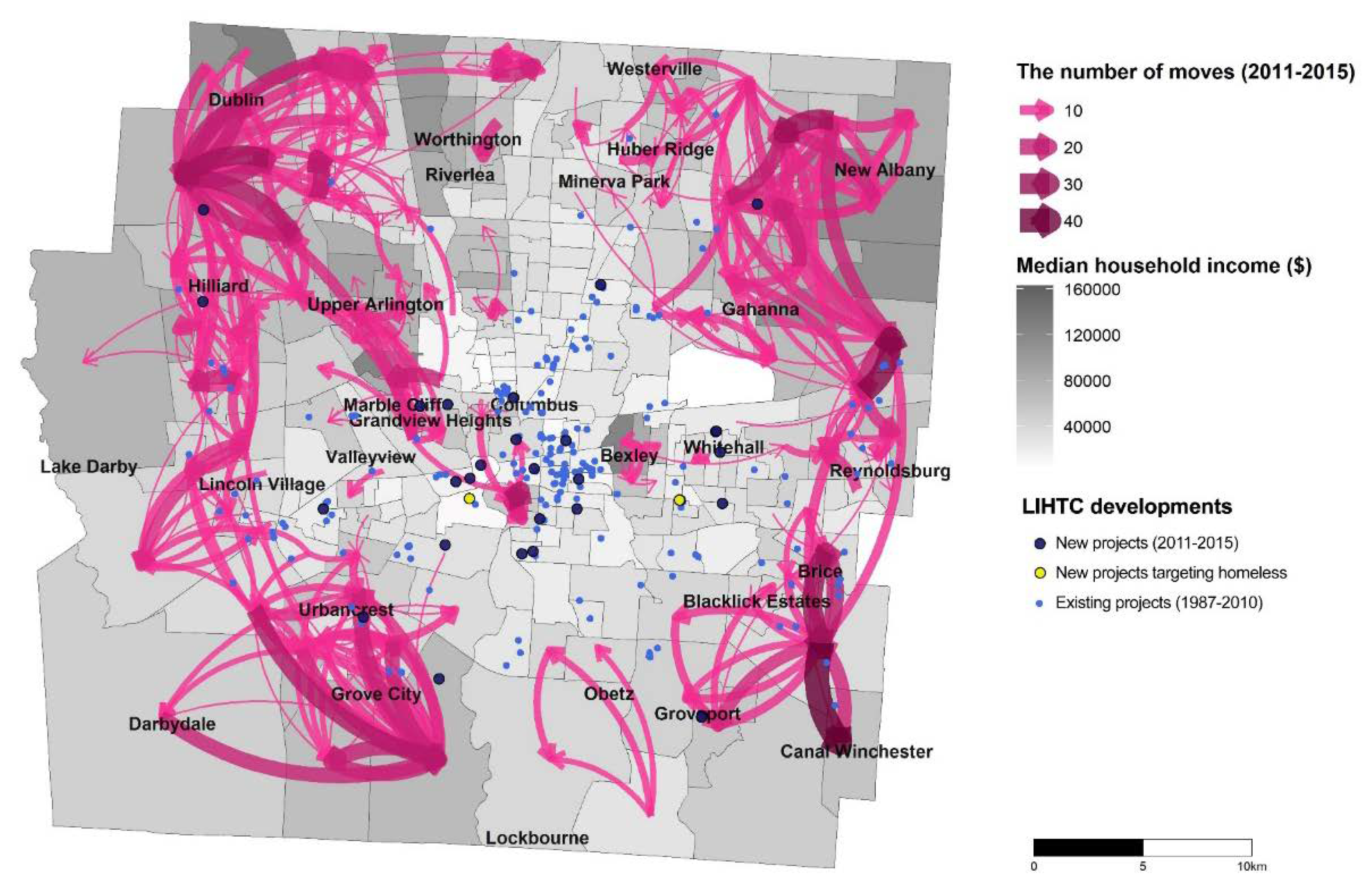
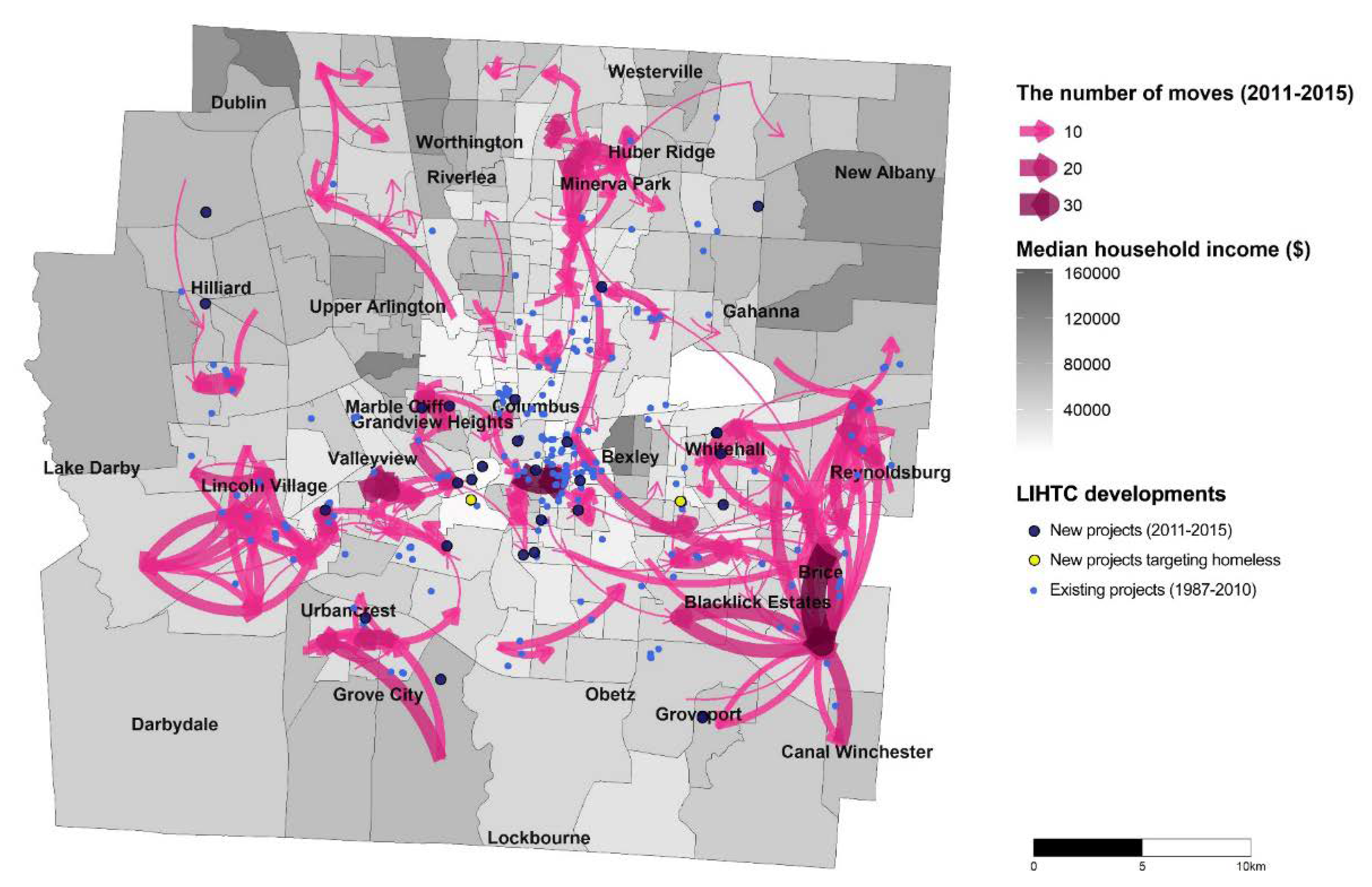
4.1. Visualization of Household Movement Patterns by Income Levels

Before we dive into gravity models, we began by visualizing household movement patterns to explore the effectiveness of new LIHTC units in attracting diverse income groups into LIHTC-deployed neighborhoods. Figure 1, Figure 2 and Figure 3 show the number of moves of the three different household income levels, high, middle, and low, respectively, in Franklin County between 2011 and 2015. The moves between census tracts higher than five were emphasized for visual clarity. The light purple dots in the maps indicate the existing locations of LIHTC projects (1987–2010), while bigger black dots represent newly developed LIHTC projects between 2011 and 2015. Around six new LIHTC projects are located in suburban neighborhoods. As shown in Figure 1, residential movements of high-income households occurred significantly within Upper Arlington, Dublin, and New Albany, which are traditionally high-income and rich suburban neighborhoods located in Franklin County. There were scarce movements of high-income households toward lower-income neighborhoods or LIHTC-deployed census tracts as demonstrated in Figure 1. Middle-income households (Figure 2) had residential mobility patterns all over the place in the suburban areas of the Franklin County. In contrast, low-income households had relatively more movements within urban core areas, including downtown Columbus, as shown in Figure 3. We also saw movement flows of low-income households to LIHTC development areas in Figure 3. Despite the wide coverage, movement destinations of low-income households were generally low-income (light grey areas) and underserved neighborhoods.

4.2. Gravity Model Results

The results of the ZINB model are summarized in

Table 2. Zero-Inflated Negative Binomial regression results.

	Variables	All Movers Estimate (SE)
Negative binomial	(Intercept)	−15.98 (0.23) ***
	Middle income	0.74 (0.02) ***
	Low income	0.74 (0.02) ***
	Number of housing unitsi (log)	1.1 (0.02) ***
	Number of housing unitsj (log)	1.11 (0.02) ***
	Physical distance (log)	−1.3 (0.02) ***
	D Share owner occupied	73.86 (4.97) ***
	Share white population	−5.04 (5.87)
	Share family with child	37.78 (4.27) ***
	Housing value (log)	18.23 (5.22) ***
	Share LIHTC units -2 years
	High income	−4.85 (0.96) ***
	Middle income	−2.46 (1.12) *
	Low income	2.04 (1.04) ***
	D2 Share owner occupied	−52.71 (4.06) ***
	Share white population	−182.54 (5.55) ***
	Share family with child	−4.79 (3.93)
	Housing value	−261.16 (7.41) ***
	Share LIHTC units -2 years
	High income	−124.88 (12.47) ***
	Middle income	−70.93 (14.58) ***
	Low income	73.35 (13.02) ***
	Existing LIHTC unitsi -2 years
	High income	−3.67 (0.35) ***
	Middle income	−0.98 (0.39) ***
	Low income	1.22 (0.37) ***
	Existing LIHTC unitsj -2 years
	High income	−11.83 (0.61) ***
	Middle income	−1.72 (0.64) ***
	Low income	1.73 (0.61) ***
	Homeless targeted LIHTCi (1 if yes)
	High income	1.67 (0.19) ***
	Middle income	0.67 (0.23) ***
	Low income	−0.08 (0.22) ***
	Homeless targeted LIHTCj (1 if yes)
	High income	2.24 (0.25) ***
	Middle income	0.7 (0.29) ***
	Low income	−0.46 (0.27) ***
	Housing stock growthj	2.65 (0.1) ***
	Neighborhood fixed effects	Yes
Logit	(Intercept)	2.85 (1.11) *
	Number of housing unitsi (log)	−0.75 (0.13) ***
	Number of housing unitsj (log)	−0.48 (0.12) ***
	Physical distance (log)	1.76 (0.13) ***
Fit statistics	Variance/mean	3.46
	Overdispersion ($\mathsf{\alpha }$)	1.36 (z = 16.5) ***
	Boundary likelihood ratio test (${\chi }^2$)	6630.2 ***
	Log Likelihood	−80,960
	AIC	163,996.2
	Observations	227,700
	Nonzero-observations (%)	23,463 (10.3%)

***, **, * denotes statistical significance at the 1%, 5% and 10% significance level.

. The overdispersion test (α) and boundary likelihood ratio test indicated that our dependent variables were overdispersed and had excessive zero counts, which justified using the ZINB over the Poisson and negative binomial models.

We found a strong positive impact of the physical distance between neighborhoods in the logit part, which revealed a strong barrier exerted by the physical distance in terms of movement possibilities. Conversely, the strong negative coefficients of the number of housing units indicated that the households moved within populous neighborhoods. Similarly, in the corresponding negative binomial portions, the distance had a significantly negative effect on the number for residential mobility. A large number of housing units contributed positively to the degree of residential mobility between two neighborhoods.

When considering socioeconomic distance variables, we found that movers were more likely to move to neighborhoods with relatively higher shares of owner-occupied homes, families with children, and higher median housing values. The share of the white population was insignificant. However, the moves were deterred by larger socioeconomic differences between the origin and destination as indicated in all of the significantly negative coefficients of squared terms of the socioeconomic distances. That is, the relationships between socioeconomic distances and the number of movers exhibited concave or inverted U-shapes, revealing that most households moved to and from neighborhoods that were alike in terms of the socioeconomic characteristics.

Regarding the control variables, negative relationships were found between the flows of high- and middle-income groups and the existing LIHTC projects, both in the origins and destinations. The higher-income groups were neither pushed out by nor pulled in by the existing LIHTC units. In contrast, there were positive relationships between low-income movers and the existing LIHTC projects in the origins and destinations, while the coefficient for a destination was slightly higher. It demonstrated that low-income movers were more likely to move to neighborhoods with existing LIHTC projects compared to other groups. Housing stock growth in destination neighborhoods significantly increased the number of move-ins.

After controlling for all of the other potential determinants, the variables of interest (the difference in the share of new LIHTC units and its squared term) indicated a linearly positive relationship with moves of low-income households. Conversely, the high-income group had a linearly negative relationship with new LIHTC projects. The middle-income group showed a similar trend as the high-income group with a lower magnitude. That is, low-income households valued neighborhoods with more new LIHTC units than those they had lived in while a higher share of new LIHTC units in destinations served as barriers to their higher-income counterparts.

4.3. Robustness Check

To check our model’s robustness, we ran the model separately for each income group. We also conducted the same analysis in Table 2 with alternative definitions of income levels and different time windows of LIHTC projects. Overall, the model appeared to be robust; the resulting coefficients and model performance tests remained qualitatively the same with minor differences in magnitude.

First, we ran the separate models for each group to examine whether the differential impact of variables that did not interact in the model reported in Table 2 on each income group changed the results (

Table 3. High-income vs. Middle-income vs. Low-income moves.

Variables	High-Income	Middle-Income	Low-Income
	Estimate (SE)	Estimate (SE)	Estimate (SE)
Negative binomial
(Intercept)	−14.71 (0.53) ***	−17.18 (0.35) ***	−14.64 (0.32) ***
Number of housing unitsi (log)	1.08 (0.05) ***	1.1 (0.03) ***	1.08 (0.03) ***
Number of housing unitsj (log)	1 (0.05) ***	1.36 (0.03) ***	0.98 (0.03) ***
Physical distance (log)	−1.61 (0.03) ***	−1.32 (0.02) ***	−1.19 (0.02) ***
D Share owner occupied	50.41 (8.21) ***	74.17 (4.55) ***	−0.31 (3.99)
Share white population	78.04 (14.22) ***	34.8 (6.08) ***	−7.77 (4.21)
Share family with child	47.31 (6.35) ***	3.03 (3.77)	−9.36 (3.64) *
Housing value (log)	105.54 (8.99) ***	16.17 (4.96) **	−50.71 (4.27) ***
Share LIHTC units ±2 years	−36.64 (10.34) ***	−14.86 (5.19) **	0.93 (3.28)
D2 Share owner occupied	−10.85 (6.47)	−19.46 (3.71) ***	−41.53 (3.35) ***
Share white population	−353.04 (18.07) ***	−147.43 (6.19) ***	−69.88 (3.8) ***
Share family with child	34.39 (5.42) ***	2.73 (3.49)	−39.51 (3.54) ***
Housing value	−155.48 (12.82) ***	−182.63 (7.82) ***	−149.94 (5.68) ***
Share LIHTC units ±2 years	−117.77 (19.22) ***	−73.51 (10.13) ***	68.11 (4.93) ***
Existing LIHTC unitsi	−2.85 (0.4) ***	−1.07 (0.17) ***	0.9 (0.1) ***
Existing LIHTC unitsj	−8.96 (0.69) ***	−0.86 (0.21) ***	1.12 (0.09) ***
Homeless targeted LIHTCi (1 if yes)	1.69 (0.22) ***	0.78 (0.13) ***	−0.1 (0.1)
Homeless targeted LIHTCj (1 if yes)	2.87 (0.3) ***	0.65 (0.15) ***	−0.02 (0.1)
Housing stock growthj	4.91 (0.23) ***	3.52 (0.15) ***	−0.15 (0.15)
Neighborhood fixed effects	Yes	Yes	Yes
Logit
(Intercept)	4.48 (3.94)	5.04 (2.59)	−0.25 (1.25)
Number of housing unitsi (log)	0.01 (0.5)	−1.32 (0.33) ***	−0.44 (0.12) ***
Number of housing unitsj (log)	−0.65 (0.42)	−0.42 (0.26)	−0.26 (0.14)
Physical distance (log)	−1.58 (0.29) ***	2.1 (0.35) ***	1.67 (0.12) ***
Fit statistics
Variance/mean	4.54	3.72	2.76
Overdispersion ($\mathsf{\alpha }$)	1.33 (z = 6.51) ***	1.24 (z = 13.52) ***	1.27 (z = 14.55) ***
Boundary likelihood ratio test (${\chi }^2$)	1532.8 ***	1587.8 ***	1835.6 ***
Log Likelihood	−13,950	−29,060	−34,200
AIC	27,760.9	58,166.9	68,459.8
Observations	75,900	75,900	75,900
Nonzero-observations (%)	3641 (4.8%)	9015 (11.9%)	10,807 (14.2%)

***, **, * denotes statistical significance at the 1%, 5% and 10% significance level.

). While the directions of socioeconomic distance variables were different from the combined model, the results supported the models with all of the income groups: new LIHTC units are preferred by low-income movers in a linearly positive shape while preventing high- and middle-income movers from moving in. It is notable that low-income groups tended to prefer neighborhoods with smaller white populations, families with children, and lower housing values, which was the opposite of the combined model. The distance variable of the white population was significantly positive for both high- and middle-income groups.

We then defined the low-income and high-income groups more strictly: (a) the low-income group was those who earned less than 60% and 50% of the county’s median household income and (b) high-income movers were those who earned 2.5 times and 3 times more than the county’s median household income (

Table 4. Robustness checks on model in Table 2.

Variables	All Movers Estimate (SE)
(a) Low-Income definition	Low-income (<67%)	Low-income (<60%)	Low-income (<50%)
D Share LIHTC units
High income	−4.85 (0.96) ***	−4.87 (0.96) ***	−4.9 (0.96) ***
Middle income	−2.46 (1.12) *	−2.72 (1.1)	−2.66 (1.09) *
Low income	2.04 (1.04) ***	2.38 (1.04) ***	2.87 (1.05) ***
D2 Share LIHTC units
High income	−124.88 (12.47) ***	−125.44 (12.48) ***	−126.4 (12.5) ***
Middle income	−70.93 (14.58) ***	−65 (14.35) ***	−57.66 (14.12) ***
Low income	73.35 (13.02) ***	77.84 (13.05) ***	84.87 (13.1) ***
(b) High-Income definition	High−income (>x2)	High−income (>x2.5)	High−income (>x3)
D Share LIHTC units
High income	−4.85 (0.96) ***	−5.74 (1.22) ***	−5.61 (1.6) ***
Middle income	−2.46 (1.12) *	−2.66 (1.34) *	−2.85 (1.69)
Low income	2.04 (1.04) ***	2.01 (1.28) ***	1.97 (1.65) ***
D2 Share LIHTC units
High income	−124.88 (12.47) ***	−151.37 (16.08) ***	−173.88 (21.83) ***
Middle income	−70.93 (14.58) ***	−72.23 (17.63) ***	−75.58 (22.93) ***
Low income	73.35 (13.02) ***	72.69 (16.51) ***	72.11 (22.14) ***
(c) Timing definition of LIHTC	±2 yr window	±1 yr window	±0 yr window
D Share LIHTC units
High income	−4.85 (0.96) ***	−5.63 (1.1) ***	−5.32 (1.5) ***
Middle income	−2.46 (1.12) *	−2.82 (1.28) *	−2.7 (1.69)
Low income	2.04 (1.04) ***	1.82 (1.18) ***	1.79 (1.57) ***
D2 Share LIHTC units
High income	−124.88 (12.47) ***	−171.91 (17.4) ***	−279.13 (25.06) ***
Middle income	−70.93 (14.58) ***	−100.93 (20.13) ***	−125.27 (28.06) ***
Low income	73.35 (13.02) ***	82.49 (17.79) ***	84.66 (25.32) ***

***, **, * denotes statistical significance at the 1%, 5% and 10% significance level.

). By doing so, we attempted to examine whether the low- and high-income groups in the final model are homogeneous in terms of mobility patterns. The results were similar in both definitions. The difference in the share of newly built LIHTCs had linearly negative associations with the flows of middle- and high-income groups and a linearly positive relationship with low-income movers. It is notable that the coefficients for the low-income group with stricter definitions were higher than that with the original definition, and the coefficients for the high-income group with stricter definitions were lower than in the model in Table 2. Furthermore, we used (c) the different definitions of newly built LIHTCs for another robustness check: ±1 year (2010–2016) and ±0 year (2011–2015) that the move occurs. The results were also similar in both cases. Regardless of the different definitions of new LIHTC projects, the difference in the share of newly built LIHTCs had a linearly negative relationship with high- and middle-income groups and a linearly positive relationship with low-income movers.

5. Discussion and Conclusions

Our empirical findings suggested that LIHTC projects influenced citywide residential mobility patterns and that the impact varied across income levels. Neighborhoods with a relatively higher share of new LIHTC units were shunned by higher-income households looking for new residences while being preferred by low-income households. Thus, new LIHTC units might have been an amenity for low-income groups while being a disamenity for higher-income groups. The results aligned with the prior study [16], which found that homebuyers purchasing properties surrounding newly completed LIHTC units had lower incomes than the local average in higher-income areas. Our analysis revealed the presence of Nimbyism against the findings of Freedman and McGavock [23]. Housing prices increased and high housing turnover in deprived neighborhoods reported in earlier studies [16,17] were likely in accordance with inflow of low-income households with a relatively higher earning, rather than part of the gentrification process [24] that replaced lower-income residents by inflow of affluent residents. The results demonstrated that new LIHTC projects, to some extent, contributed to alleviating poverty concentration in lower-income neighborhoods, but that their contribution to income mixing was questionable because higher-income households are less likely to move into neighborhoods with new LIHTC projects. In our analysis, however, the existing LIHTC projects did not necessarily function as a push factor for middle- and high-income groups, although they were not pulled into neighborhoods with a higher share of existing LIHTC units. While the results were possibly compounded by the concentrated location of LIHTC units in lower-income neighborhoods, the results suggested that LIHTC units did not push higher-income households out of the neighborhood in the long term. In that sense, it calls for continued efforts to alleviate immediate opposition to new LIHTC developments, especially in affluent neighborhoods (i.e., creative design approaches, campaigns, and mixed-income units).

Regardless of income level, households moved to affluent neighborhoods with more homeowners and higher housing values in addition to a preference toward neighborhoods with similar socioeconomic characteristics as those they used to live in. These results supported and were well-aligned with existing arguments that residential mobility is largely restricted by budget and housing market conditions [65,66], with a greater degree of homophily (i.e., the tendency for people to be attracted to those who are similar to themselves) [57,67]. The results also suggested the presence of underlying structural barriers sorting income groups into specific neighborhoods.

Our analysis had several limitations that must be addressed in future studies. First, the moves of low-income households include the moves of LIHTC tenants, which possibly exacerbates the positive impacts of new LIHTC developments on the low-income group. Second, the model did not capture the dynamics of neighborhood changes during the time period of interest. While we assumed that there were no substantial changes in neighborhoods to avoid endogeneity problems in our gravity models, there could have been an interdependent impact of mobility on neighborhoods. In particular, a trend of gentrification and depreciation could have compounded the impact of LIHTC units predominantly located in lower-income neighborhoods. Third, census tracts, a spatial unit of the analysis, might have been too large to examine LIHTC’s impact on the surrounding neighborhood. In earlier studies, less than one mile around LIHTC units was defined as a neighborhood [9,17]. Future work will require a more sophisticated method of operationalizing LIHTC variables with more disaggregated datasets and linking them to intrinsic characteristics of housing as well as to micro-surroundings. Lastly, although our results were robust, this study may not be generalizable to other US cities across time. We suggest that future studies need to conduct a panel analysis to examine whether the patterns discovered in the analysis were consistent across time and to explore other cities, LIHTC contexts, and household types.

Nevertheless, this study offers two significant academic contributions. First, from a methodological perspective, we demonstrate that gravity models can be useful for understanding residential mobility patterns within a smaller geographical scale, such as a neighborhood or city. Our study adds empirical evidence for using gravity models to analyze intra-urban residential mobility, considering the interdependent relationship between the origin and destination. Second, this study provides evidence that the current LIHTC housing policy impacts, heterogeneously, peoples’ decisions to move by income level, and therefore does not necessarily induce the creation of mixed-income neighborhoods that is one of the main goals of US affordable housing policies [7]. Our analytical approach offers a scientific framework to understand the impact of place-based housing policy on household movement and neighborhood dynamics, thereby helping city officials, policymakers, and planners to formulate supplemental programs and strategies to overcome the current housing policy’s shortcomings.

References

1. Bischoff, K.; Reardon, S.F. Residential Segregation by Income, 1970–2009. In Diversity and Disparities: America Enters a New Century; Logan, J., Ed.; The Russell Sage Foundation: New York, NY, USA, 2014; pp. 208–233. [Google Scholar]
2. Florida, R. The New Urban Crisis: How Our Cities Are Increasing Inequality, Deepening Segregation, and Failing the Middle Class—And What We Can Do about It; Basic Books: New York, NY, USA, 2017. [Google Scholar]
3. Chaskin, R.J.; Joseph, M.L. “Positive” Gentrification, Social Control and the “Right to the City” in Mixed-Income Communities: Uses and Expectations of Space and Place. Int. J. Urban Reg. Res. 2013, 37, 480–502. [Google Scholar] [CrossRef] [Green Version]
4. Lees, L.; Ley, D. Introduction to Special Issue on Gentrification and Public Policy. Urban Stud. 2008, 45, 2379–2384. [Google Scholar] [CrossRef]
5. OECD. Social Housing: A Key Part of Past and Future Housing Policy. In Employment, Labour and Social Affairs Policy Briefs; OECD: Paris, France, 2020; pp. 1–32. [Google Scholar]
6. Popkin, S.J.; Cunningham, M.K.; Burt, M. Public Housing Transformation and the Hard-to-House. Hous. Policy Debate 2005, 16, 1–24. [Google Scholar] [CrossRef]
7. McClure, K. What Should Be the Future of the Low-Income Housing Tax Credit Program? Hous. Policy Debate 2019, 29, 65–81. [Google Scholar] [CrossRef]
8. Texas Low Income Housing Information. In Fair Housing and Balanced Choices: Did Texas Reduce Government—Funded Segregation? Texas Housers: Houston, TX, USA, 2017.
9. Baum-Snow, N.; Marion, J. The Effects of Low Income Housing Tax Credit Developments on Neighborhoods. J. Public Econ. 2009, 93, 1–7. [Google Scholar] [CrossRef] [PubMed] [Green Version]
10. Ellen, I.G.; O′Regan, K.M.; Voicu, I. Siting, Spillovers, and Segregation: A Reexamination of the Low Income Housing Tax Credit Program. In Housing Markets and the Economy: Risk, Regulation, and Policy; Glaeser, E.L., Quigley, J.M., Eds.; Lincoln Institute of Land Policy: Cambridge, UK, 2009. [Google Scholar]
11. DeLuca, S.; Garboden, P.M.E.; Rosenblatt, P. Segregating Shelter: How Housing Policies Shape the Residential Locations of Low-Income Minority Families. Ann. Am. Acad. Pol. Soc. Sci. 2013, 647, 268–299. [Google Scholar] [CrossRef]
12. South, S.J.; Crowder, K.D. Residential Mobility Between Cities and Suburbs: Race, Suburbanization, and Back-to-the-City Moves. Demography 1997, 34, 525. [Google Scholar] [CrossRef] [PubMed]
13. Greenlee, A.J. Assessing the Intersection of Neighborhood Change and Residential Mobility Pathways for the Chicago Metropolitan Area (2006–2015). Hous. Policy Debate 2019, 29, 186–212. [Google Scholar] [CrossRef]
14. Boggs, E. People and Place in Low-Income Housing Policy—Unwinding Segregation in Connecticut. Hous. Policy Debate 2017, 27, 320–326. [Google Scholar] [CrossRef]
15. Horn, K.M.; O′Regan, K.M. The Low Income Housing Tax Credit and Racial Segregation. Hous. Policy Debate 2011, 21, 443–473. [Google Scholar] [CrossRef] [Green Version]
16. Diamond, R.; McQuade, T. Who Wants Affordable Housing in Their Backyard? An Equilibrium Analysis of Low-Income Property Development. J. Polit. Econ. 2019, 127, 1063–1117. [Google Scholar] [CrossRef] [Green Version]
17. Woo, A.; Joh, K.; Van Zandt, S. Unpacking the Impacts of the Low-Income Housing Tax Credit Program on Nearby Property Values. Urban Stud. 2016, 53, 2488–2510. [Google Scholar] [CrossRef]
18. Khadduri, J.; Climaco, C.; Burnett, K.; Gould, L.; Elving, L. What Happens to Low-Income Housing Tax Credit Properties at Year 15 and Beyond? U.S. Department of Housing and Urban Development: Washington, DC, USA, 2012.
19. Dillman, K.N.; Horn, K.M.; Verrilli, A. The What, Where, and When of Place-Based Housing Policy’s Neighborhood Effects. Hous. Policy Debate 2017, 27, 282–305. [Google Scholar] [CrossRef]
20. Lang, B.J. Location Incentives in the Low-Income Housing Tax Credit: Are Qualified Census Tracts Necessary? J. Hous. Econ. 2012, 21, 142–150. [Google Scholar] [CrossRef]
21. Casey, C.; Moulton, S. Coproduction of Public Values through Cross-Sector Implementation: A Multilevel Analysis of Community Reinvestment Outcomes in the Low-Income Housing Tax Credit Program. In Creating Public Value in Practice; Bryson, J.M., Crosby, B.C., Bloomberg, L., Eds.; Routledge: New York, USA, 2015; pp. 163–181. [Google Scholar] [CrossRef]
22. Schwartz, A.F. Housing Policy in the United States; Routledge: New York, NY, USA, 2014. [Google Scholar]
23. Freedman, M.; McGavock, T. Low-Income Housing Development, Poverty Concentration, and Neighborhood Inequality. J. Policy Anal. Manag. 2015, 34, 805–834. [Google Scholar] [CrossRef]
24. Woo, A.; Joh, K.; Van Zandt, S. Impacts of the Low-Income Housing Tax Credit Program on Neighborhood Housing Turnover. Urban Aff. Rev. 2016, 52, 247–279. [Google Scholar] [CrossRef]
25. Freeman, L. Siting Affordable Housing: Location and Neighborhood Trends of Low Income Housing Tax Credit Developments in the 1990s; The Brookings Institution: Washington, DC, USA, 2004. [Google Scholar]
26. Schwartz, A.E.; Ellen, I.G.; Voicu, I.; Schill, M.H. The External Effects of Place-Based Subsidized Housing. Reg. Sci. Urban Econ. 2006, 36, 679–707. [Google Scholar] [CrossRef]
27. Koschinsky, J. Spatial Heterogeneity in Spillover Effects of Assisted and Unassisted Rental Housing. J. Urban Aff. 2009, 31, 319–347. [Google Scholar] [CrossRef]
28. Lee, C.-M.; Culhane, D.P.; Wachter, S.M. The Differential Impacts of Federally Assisted Housing Programs on Nearby Property Values: A Philadelphia Case Study. Hous. Policy Debate 1999, 10, 75–93. [Google Scholar] [CrossRef] [Green Version]
29. Freedman, M.; Owens, E.G. Low-Income Housing Development and Crime. J. Urban Econ. 2011, 70, 115–131. [Google Scholar] [CrossRef]
30. Lens, M.C. Subsidized Housing and Crime. J. Plan. Lit. 2013, 28, 352–363. [Google Scholar] [CrossRef] [Green Version]
31. Eriksen, M.D.; Rosenthal, S.S. Crowd out Effects of Place-Based Subsidized Rental Housing: New Evidence from the LIHTC Program. J. Public Econ. 2010, 94, 953–966. [Google Scholar] [CrossRef]
32. Nguyen, M.T. Does Affordable Housing Detrimentally Affect Property Values? A Review of the Literature. J. Plan. Lit. 2005, 20, 15–26. [Google Scholar] [CrossRef]
33. McClure, K. The Low-income Housing Tax Credit Program Goes Mainstream and Moves to the Suburbs. Hous. Policy Debate 2006, 17, 419–446. [Google Scholar] [CrossRef]
34. McClure, K.; Johnson, B. Housing Programs Fail to Deliver on Neighborhood Quality, Reexamined. Hous. Policy Debate 2015, 25, 463–496. [Google Scholar] [CrossRef]
35. Reece, J.; Rogers, C.; Martin, M.; Colombo, L.; Holley, D.; Lindsjo, M. Neighborhoods & Community Development in Franklin County; The Community Development Collaborative of Greater Columbus: Columbus, OH, USA, 2012. [Google Scholar]
36. Rosenberg, G. Same City, Different Worlds. 2017. Available online: https://www.pbs.org/wnet/chasing-the-dream/stories/city-different-worlds/ (accessed on 12 October 2021).
37. Lee, J.; Irwin, N.; Irwin, E.; Miller, H.J. The Role of Distance-Dependent Versus Localized Amenities in Polarizing Urban Spatial Structure: A Spatio-Temporal Analysis of Residential Location Value in Columbus, Ohio, 2000–2015. Geogr. Anal. 2020, 53, 283–306. [Google Scholar] [CrossRef]
38. Affordable Housing Alliance Central Ohio. The Columbus and Franklin County Affordable Housing Challenge: Needs, Resources, and Funding Models; Affordable Housing Alliance Central Ohio: Columbus, OH, USA, 2017. [Google Scholar]
39. Grady, B.P.; Boos, C.J. Qualified Allocation Plans as an Instrument of Mixed-Income Placemaking. In What Works to Promote Inclusive, Equitable Mixed-Income Communities; Joseph, M.L., Khare, A.T., Eds.; Federal Reserve Bank of San Francisco: San Francisco, CA, USA, 2020. [Google Scholar]
40. Data Axle. U.S. Historical Business Database (Archive Year 2011 and 2015); Data Axle: Dallas, TX, USA, 2021. [Google Scholar]
41. Pan, H.; Chen, S.; Gao, Y.; Deal, B.; Liu, J. An Urban Informatics Approach to Understanding Residential Mobility in Metro Chicago. Environ. Plan. B Urban Anal. City Sci. 2020, 47, 1456–1473. [Google Scholar] [CrossRef]
42. Wang, Y.; Lee, B.; Greenlee, A. The Role of Smart Growth in Residential Location Choice: Heterogeneity of Location Preferences in the Chicago Region. J. Plan. Educ. Res. 2021. [Google Scholar] [CrossRef]
43. U.S. Census Bureau. 2010 Census; U.S. Census Bureau: Suitland, MD, USA, 2010.
44. Kennel, T.L.; Li, M.; Bureau, U.S.C.; Road, S.H. Content and Coverage Quality of a Commercial Address List as a National Sampling Frame for Household Surveys. In Proceedings of the Joint Statistical Meetings 2009, Washington, DC, USA, 1– August 2009; pp. 2364–2378. [Google Scholar]
45. Lee, K.O.; Smith, R.; Galster, G. Subsidized Housing and Residential Trajectories: An Application of Matched Sequence Analysis. Hous. Policy Debate 2017, 27, 843–874. [Google Scholar] [CrossRef]
46. Nilsson, I.; Delmelle, E.C. Impact of New Rail Transit Stations on Neighborhood Destination Choices and Income Segregation. Cities 2020, 102, 102737. [Google Scholar] [CrossRef]
47. Cadwallader, M. Migration and Residential Mobility: Macro and Micro Approached; The University of Wisconsin Press: Madison, WI, USA, 1992. [Google Scholar]
48. Bakens, J.; Florax, R.J.G.M.; Mulder, P. Ethnic Drift and White Flight: A Gravity Model of Neighborhood Formation. J. Reg. Sci. 2018, 58, 921–948. [Google Scholar] [CrossRef] [Green Version]
49. Kochhar, R. The American Middle Class Is Stable in Size, But Losing Ground Financially to Upper-Income Families. Available online: https://www.pewresearch.org/fact-tank/2018/09/06/the-american-middle-class-is-stable-in-size-but-losing-ground-financially-to-upper-income-families/ (accessed on 7 September 2021).
50. U.S. Census Bureau. 2007–2011 ACS 5-Year Estimates; U.S. Census Bureau: Suitland, MD, USA, 2011.
51. Bucholtz, S.; Molfino, E.; Kolko, J. The Urbanization Perceptions Small Area Index: An Application of Machine Learning and Small Area Estimation to Household Survey Data; U.S. Department of Housing and Urban Development: Washington, DC, USA, 2020.
52. Karemera, D.; Oguledo, V.I.; Davis, B. A Gravity Model Analysis of International Migration to North America. Appl. Econ. 2000, 32, 1745–1755. [Google Scholar] [CrossRef]
53. Quigley, J.M.; Weinberg, D.H. Intra-Urban Residential Mobility: A Review and Synthesis. Int. Reg. Sci. Rev. 1977, 2, 41–66. [Google Scholar] [CrossRef] [Green Version]
54. Poot, J.; Alimi, O.; Cameron, M.P.; Maré, D.C. The Gravity Model of Migration: The Successful Comeback of an Ageing Superstar in Regional Science; Institute for the Study of Labor: Bonn, Germany, 2016. [Google Scholar]
55. Fagiolo, G.; Mastrorillo, M. International Migration Network: Topology and Modeling. Phys. Rev. E 2013, 88, 012812. [Google Scholar] [CrossRef]
56. Torrens, P.M. A Geographic Automata Model of Residential Mobility. Environ. Plan. B Plan. Des. 2007, 34, 200–222. [Google Scholar] [CrossRef] [Green Version]
57. van Ham, M.; Feijten, P. Who Wants to Leave the Neighbourhood? The Effect of Being Different from the Neighbourhood Population on Wishes to Move. Environ. Plan. A 2008, 40, 1151–1170. [Google Scholar] [CrossRef] [Green Version]
58. Britton, M.L.; Goldsmith, P.R. Keeping People in Their Place? Young-Adult Mobility and Persistence of Residential Segregation in US Metropolitan Areas. Urban Stud. 2013, 50, 2886–2903. [Google Scholar] [CrossRef]
59. Rosenblatt, P.; Deluca, S. “We Don’t Live Outside, We Live in Here”: Neighborhood and Residential Mobility Decisions Among Low-Income Families. City Community 2012, 11, 254–284. [Google Scholar] [CrossRef]
60. Liu, L.; Feng, J.; Ren, F.; Xiao, L. Examining the Relationship between Neighborhood Environment and Residential Locations of Juvenile and Adult Migrant Burglars in China. Cities 2018, 82, 10–18. [Google Scholar] [CrossRef]
61. Liu, Y.; Shen, J. Spatial Patterns and Determinants of Skilled Internal Migration in China, 2000–2005. Pap. Reg. Sci. 2014, 93, 749–771. [Google Scholar] [CrossRef]
62. Greene, J. Accounting for Excess Zeros and Sample Selection in Poisson and Negative Binomial Regression Models. NYU Work. Pap. 1994, 9, 265. [Google Scholar]
63. Wilson, P. The Misuse of the Vuong Test for Non-Nested Models to Test for Zero-Inflation. Econ. Lett. 2015, 127, 51–53. [Google Scholar] [CrossRef] [Green Version]
64. Young, D.S.; Raim, A.M.; Johnson, N.R. Zero-Inflated Modelling for Characterizing Coverage Errors of Extracts from the US Census Bureau’s Master Address File. J. R. Stat. Soc. Ser. A Stat. Soc. 2017, 180, 73–97. [Google Scholar] [CrossRef]
65. Clark, W.A.V.; Coulter, R. Who Wants to Move? The Role of Neighbourhood Change. Environ. Plan. A 2015, 47, 2683–2709. [Google Scholar] [CrossRef] [Green Version]
66. Coulter, R.; Van Ham, M.; Findlay, A. New Directions for Residential Mobility Research: Linking Lives through Time and Space; Institute for the Study of Labor: Bonn, Germany, 2013; p. 7525. [Google Scholar]
67. Schelling, T. Models of Segregation. Am. Econ. Rev. 1969, 59, 488–493. [Google Scholar]
Figure 1. High-income households’ residential mobility in Franklin County, Ohio, 2011–2015. Source: calculations based on Data Axle [40].
Urbansci 05 00079 g001
Figure 2. Middle-income households’ residential mobility in Franklin County, Ohio, 2011–2015. Source: calculations based on Data Axle [40].
Urbansci 05 00079 g002
Figure 3. Low-income households’ residential mobility in Franklin County, Ohio, 2011–2015. Source: calculations based on Data Axle [40].
Urbansci 05 00079 g003