
Industry Interconnectedness and Regional Economic Growth in Germany


1
School of Complex Adaptive Systems, Arizona State University, Tempe, AZ 85287, USA
2
Global Climate Forum, 10178 Berlin, Germany
3
Institute for Employment Research, 10969 Berlin, Germany
4
Embassy of the Federal Republic of Germany, Washington, DC 20007, USA
5
School of Complex Adaptive Systems, Arizona State University, Washington, DC 20006, USA
*
Author to whom correspondence should be addressed.
Urban Sci. 2022, 6(1), 1; https://0-doi-org.brum.beds.ac.uk/10.3390/urbansci6010001
Submission received: 16 November 2021
/
Revised: 10 December 2021
/
Accepted: 16 December 2021
/
Published: 21 December 2021
(This article belongs to the Special Issue Feature Papers in Urban Science)
Abstract
:Urban systems, and regions more generally, are the epicenters of many of today’s social issues. Yet they are also the global drivers of technological innovation, and thus it is critical that we understand their vulnerabilities and what makes them resilient to different types of shocks. We take regions to be systems composed of internal networks of interdependent components. As the connectedness of those networks increases, it allows information and resources to move more rapidly within a region. Yet, it also increases the speed and efficiency at which the effects of shocks cascade through the system. Here we analyzed regional networks of interdependent industries and how their structures relate to a region’s vulnerability to shocks. Methodologically, we utilized a metric of economic connectedness called tightness which quantifies a region’s internal connectedness relative to other regions. We calculated tightness for German regions during the Great Recession, comparing it to each region’s economic performance during the shock (2007–2009) and during recovery (2009–2011). We find that tightness is negatively correlated with changes in economic performance during the shock but positively during recovery. This suggests that regional economic planners face a tradeoff between being more productive or being more vulnerable to the next economic shock.
1. Introduction
Many of today’s pressing social, economic, and ecological issues are focused in urban systems [1,2]. They are epicenters of pollution, crime, inequality, and health problems. Yet urban systems are also epicenters of creativity. They are the global drivers of innovation and productivity that fuel the global economy and the emergence of new technologies [3,4]. Being the focal point of so many social, ecological, and economic forces makes the management of regions extremely difficult. More importantly, urban systems are embedded within regions, with which they share an integrated economy, workforce, and other key attributes. Thus, our focus in this paper is not specifically on urban systems, but on regions more broadly.
This complexity of regions has often been an obstacle to understanding and guiding regions and has resulted in policy interventions that have unintended and sometimes negative consequences [5]. Fortunately, complexity science has begun to mature to the point that it is enabling researchers to move beyond lingering obstacles to a fundamental understanding of regional systems. Here we adopt the framework that regions are complex adaptive systems [6,7,8] and that they exhibit a key attribute of such systems, namely internal networks of interdependent components [9,10,11]. As the internal connectedness of those networks increases, it can impact the ability of information and resources to move more rapidly and efficiently within a region. Yet, it also increases the speed and efficiency at which the effects of shocks cascade through the system.
In this study we focus on regional networks of interdependent economic components and how their structures relate to a region’s vulnerability to shocks. To do so, we utilized a metric of economic connectedness, known as tightness, which attempts to quantify the rather ambiguous notion of a region’s aggregate degree of internal interdependencies relative to other regions. Previously, this measure has only been analyzed in United States (U.S.) metropolitan areas [12,13,14] and has shown that regional tightness is positively correlated with more severe declines in economic performance following a shock [12]. Thus, economic tightness is intimately linked to resilience and its importance lay in its potential ability to help anticipate impacts of system shocks, particularly economic shocks.
In our empirical analysis, we focus on Europe’s biggest economy, Germany, for various reasons. First, the country has emerged as one of the most resilient economies following thorough labor market and structural reforms at the beginning of the 21st century. Its gains in competitiveness vis-à-vis countries such as France, Italy, and Spain suggest that it was not the depreciation of the Euro that served as the key driver of the German economy, but that it was Germany’s high relative productivity gains [15].
Our study focuses on another potential factor behind the economic success of Germany, the sectoral connectedness as a proxy for the strengths of regional supply chains as well as networks and thus important parameters for resilience. Second, regional disparities in Germany, even if decreasing between West and East Germany after the reunification of both parts in 1990, still persist [16] and were used as a justification for allocating more than EUR 45 billion for investment subsidies as the main instrument of German regional policy over the last 30 years [17]. Our analytical approach allows us to explore whether an increase in regional economic connectedness could lead to a decrease in regional disparities.
Finally, because German labor market regions (LMRs) cover all of Germany, they provide a valuable contrast to studies of U.S. metropolitan statistical areas, which cover only larger, urbanized areas of the U.S. In essence this permits a contrast of urban systems with regional systems.
While others have used skills data to analyze resilience of a single German state [18], here we use industry employment data to calculate the economic tightness of all 141 German LMRs. We then compare that metric to each region’s economic performance both during the shock (2007–2009) and during the subsequent recovery (2009–2011). Using per worker GDP as a measure of economic performance, we find that tightness is negatively correlated with changes in economic performance during the shock but positively correlated with the same indicator during recovery. In other words, regions with tighter economies suffered more severely during a shock but had larger growth rates in the absence of a shock.
Based on the latest available employment statistics of the Federal Employment Agency (Bundesagentur für Arbeit), we also analyze the potential relationship between economic tightness and employment development of German labor market regions in the first months of the COVID-19 pandemic. We observe that tightness seemed to play a significant role in regional economic development. This was true even though supply and demand impacts of the pandemic affected the German economy significantly more symmetrically than the 2007–2009 Great Recession as it impacted public life and therefore wide parts of the service and retail trade sector.
These overall results support the notion that economic interdependence can make regions more economically productive but also more precarious. This result concurs with the so-called Panarchy theory of complex adaptive systems [19,20,21], which asserts that systems with higher internal connectedness are more efficient, but also more brittle and vulnerable to disruption. Thus, regional economic planners must navigate a tradeoff between being more productive or being more vulnerable to the next economic shock [7,22].
2. Materials and Methods
2.1. Data and Sources
We performed our analyses on two types of geographical units. The first are Germany’s 401 districts (Landkeise and kreisfreie Städte) which comprise the Nomenclature of Territorial Units for Statistics (NUTS 3) regions of Germany. These units are roughly analogous to U.S. counties, and thus we refer to these 401 smaller units as counties hereafter. The second geographical units of analysis are the 141 labor market regions (LMRs) of Germany as defined by Kosfeld and Werner [23]. LMRs are aggregations of one or more counties having close commuter links with each other and are considered to be essentially independent economic units. Each German county is a part of one and only one LMR.
Industry employment data were supplied by Germany’s Institute for Employment Research (Institut für Arbeitsmarkt- und Berufsforschung—IAB) at the county level. Employment was analyzed at both 3-digit and 4-digit industry code aggregation levels. LMR-level employment was aggregated from county-level employment data. While employment could be further aggregated to 2-digit industry level, variance of interdependence values becomes too small and industries become too ubiquitous to offer meaningful insights.
To assess regional economic performance, we used regional gross domestic product (GDP) per capita. These estimates are taken from Federal Statistical Office (Destatis) data at the county level and aggregated to LMRs.
2.2. Quantifying Interdependence, a Pairwise Measure of Industry Interdependence
To quantify an aggregate measure of interdependence characterizing each LMR’s economy, we first determined which industries are present or absent in each LMR. While a region may have employment in many industries, we used a threshold of relative abundance to determine presence or absence for our analysis. We applied the traditional metric of location quotient (LQ):
where e is the employment in industry i in LMA m. Thus, LQ—also known as Revealed Comparative Advantage or RCA—is a region’s proportion of employment in i compared to the national proportion. Following [24] we take an industry i to be present in LMR m if LQi,m ≥ 1 and absent if LQi,m < 1. This results in an LMR × industry matrix of presence–absence data.
This matrix was then used to calculate the probability that two industries i and j will co-occur in a random LMR. Using a variant of mutual information defined in [24] we quantify the interdependence x between any two industries i and j as
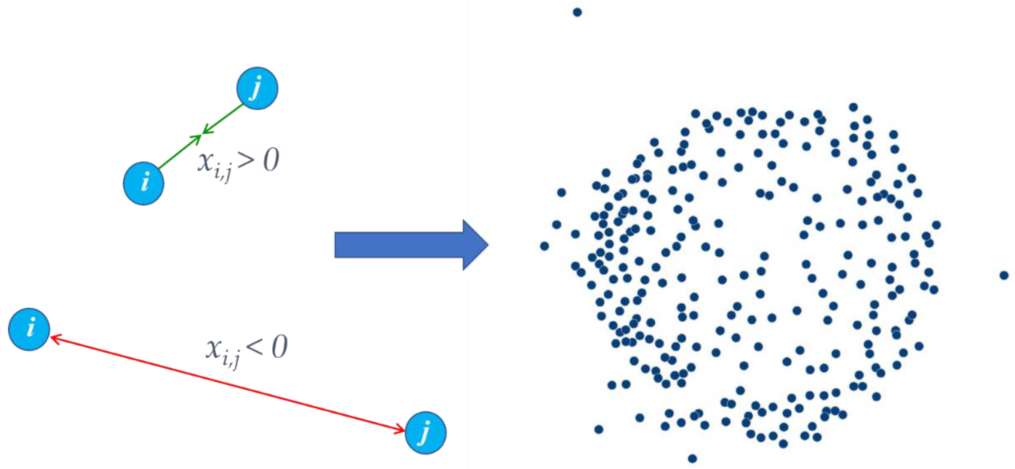
where m, m′, and m″ denote randomly selected LMRs. The result is an industry × industry matrix of interdependence values. Two industries that co-occur in LMRs more frequently than expected by chance will have a positive interdependence value, while two industries that co-occur less frequently than expected will have negative interdependence. We take this matrix of interdependence values to be the adjacency matrix of a complete, weighted network describing how industries interact across Germany. Note that xi,j = xj,i so that the adjacency matrix is symmetric and the resulting network is thus undirected.
2.3. Quantifying Tightness, a Regional Aggregate Measure of Industry Interdependence
Using the methodology outlined in [12] we then calculated an aggregate measure of LMR interdependence, or tightness. This method dictates that we first assign an LMR-specific weight L to each pair of industries present in an LMR using the national-level pairwise interdependence x and weighting by the local proportions of employment in each industry:
where i and j are industries that are both present in LMR m. We then average L across the total number of links in an LMR’s industry subnetwork to produce an industry-based tightness metric:
where i and j are both present in LMR and Nm is the total number of industries present in LMR m. Note that averaging the weight L across all links in an LMR’s subnetwork is equivalent to the generalized formula of network density [25,26]. Because tightness is a dimensionless measure, we normalize tightness values across LMRs as a z-score with mean of 0 and standard deviation of 1.
2.4. Designation of Time Periods
To understand the role of tightness in the economic performance of German regions, we correlate tightness with two time periods related to the global Great Recession. While any division of this recession may be somewhat arbitrary, we designate the shock period as 2007–2009. This period was chosen as a large year-over-year decrease in both GDP and employment was experienced from 2007 to 2008, while economic indicators began to increase after 2009 [27].
We then designated the period 2009–2011 as the recovery period for Germany. Again, while one may argue that this is somewhat arbitrary, unlike most other countries of Europe, Germany returned to its pre-recession level of GDP in 2011 [28], and thus we use this year as the end of our designated recovery period.
2.5. Empirical Treatments
The methodology described thus far applies to data for a specific year, industry aggregation level, and spatial unit. To examine the effects of industry aggregation level, we calculated interdependence using employment data aggregated to both 3-digit (N = 270) and 4-digit (N = 604) industry levels. To better understand the effect of different regional definitions, we also calculated interdependence using both LMRs (N = 141) and counties (N = 401).
Thus, for a given year we constructed four interdependence matrices using a 2 × 2 treatment approach. Finally, we replicated this 2 × 2 treatment using both 2007 and 2009 data for a total of eight interdependence matrices (industry level × area type × year). As our goal is to understand the relationship between economic tightness and regional vulnerability, years were chosen to correspond to points in time at the beginning of the 2007–2009 global recessions and at the beginning of the recovery period.
3. Results and Discussion
3.1. Industry Interdependence
To calculate the economic tightness of LMRs, we first calculated an interdependence value for all possible pairs of industries. Industry pairs that tend to appear together in the same LMRs will have higher interdependence than pairs that rarely occur together. Industry pairs that occur together less frequently than expected by chance will have a negative interdependence value.
Interdependence is a nuanced metric that captures elements of relatedness as defined by Frenken et al. [29] and subsequently adopted by others [30,31,32]. Frenken’s relatedness captures linkages between industries sharing similar industry codes in the German industry classification system. Thus, some industry pairs with high interdependence values also have high relatedness values, such as “Mining of hard coal” and “Manufacture of coke oven products”, which have the highest interdependence of any industry pair with x = 22.5 using 2007 3-digit industry employment at the LMR level.
On the other hand, some highly interdependent pairs are seemingly unrelated in the Frenken sense, such as “Passenger air transport” and “Fund management activities” with x = 19.1. Thus, interdependence can also capture so-called Marshallian externalities [33,34,35,36]. These industries are related because they share common labor requirements, natural resource inputs, customers, etc.
3.2. The German Industry Network
Calculating interdependence between all industry pairs results in an industry × industry matrix of interdependence values. This matrix is taken to be the adjacency matrix of a complete and weighted national-level industry network, in which nodes are industries and weights are pairwise interdependence values. The resulting network, shown in Figure 1, was created using MATLAB’s nonclassical multidimensional scaling function mdscale [37]. Industry pairs that are highly interdependent tend to be near each other in this network, while pairs with a low or negative interdependence tend to be farther apart.
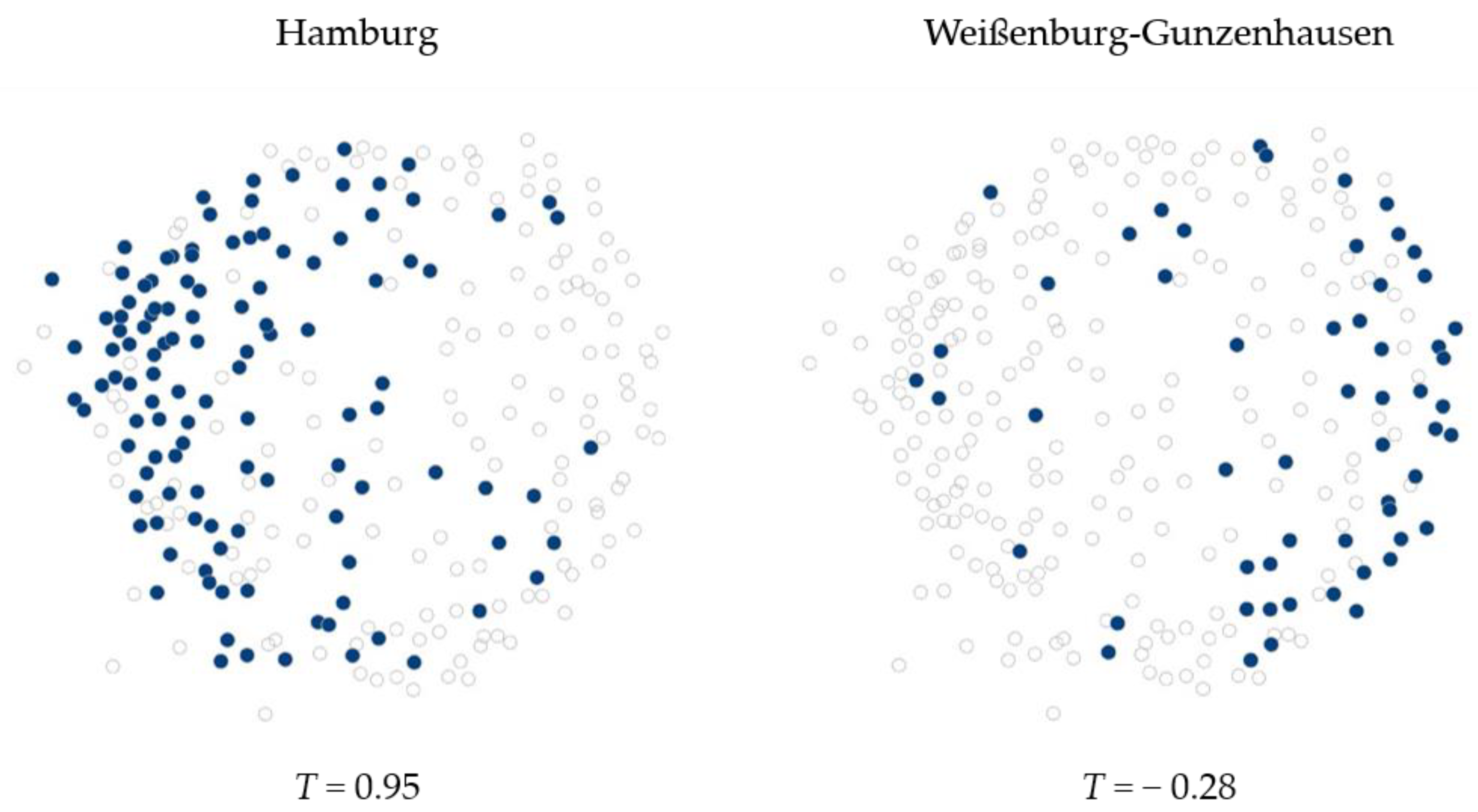
In any LMR there exists only a subset of all possible industries. This industry portfolio represents an economic signature of the LMR and can be shown as a subnetwork of the national-level interdependence network. We take this subnetwork to be the “location” of a an LMR within a national map. Examples of two LMR subnetworks are shown in Figure 2. These examples demonstrate visually the concept of tightness as nodes are clustered more closely together in the LMR with higher tightness (Hamburg) and more dispersed in the region with lower tightness (Weißenburg-Gunzenhausen).
The network shown in Figure 1 and Figure 2 was constructed with 2007 employment data at the 3-digit industry level for 141 LMRs. Though not shown, we also constructed networks for each of the other combinations of year, industry aggregation level, and spatial unit, as described in the empirical treatments of the methods section. Thus, we ultimately created eight national industry interdependence networks (2007/2009, 3-/4-digit industry code, 141 LMRs/401 counties).
3.3. LMRs and Tightness
Applying industry interdependence values to the eight networks described in the previous section, we then located the subnetwork of every German spatial unit within the corresponding network and calculated its tightness T. A list of LMRs having highest and lowest 2007 tightness values using 3-digit industry data is presented in Table 1.
The distribution of tightness values across regions is highly skewed with only four regions being more than two standard deviations from the mean T value. The highest level of interconnectedness in the LMR Wolfsburg is due to the high importance of the automotive industry there, which is much more pronounced in this region than in any other German LMR. Approximately one third of all employees in and around Wolfsburg work in the automotive and automotive supplier industries in 2008. Employee leasing, accounting for 6 percent of all employees, may also play a role here.
As the capital region, Berlin is strongly characterized by employment in political interest groups, but also in information technology services, universities and research institutes, as well as credit institutes. The Frankfurt am Main region is Germany’s central banking district. In addition, many employees in aviation, management consultancies are concentrated here. The regions of Frankfurt an der Oder and Cottbus are characterized by larger shares of employment in steel production and lignite mining, respectively, and power generation (coal-fired). Both sectors are characterized by significant direct and indirect employment effects on other economic sectors in the region and beyond.
LMRs at the lower end of the tightness table, on the other hand, are predominantly characterized by public-sector industries such as hospitals, geriatric care, social services, public administration, and retail. In addition, the five regions feature singular concentrated manufacturing industries that appear to have fewer links to other industries, such as furniture manufacturing and plastic goods manufacturing.
3.4. Spatial Distribution and Autocorrelation of Tightness
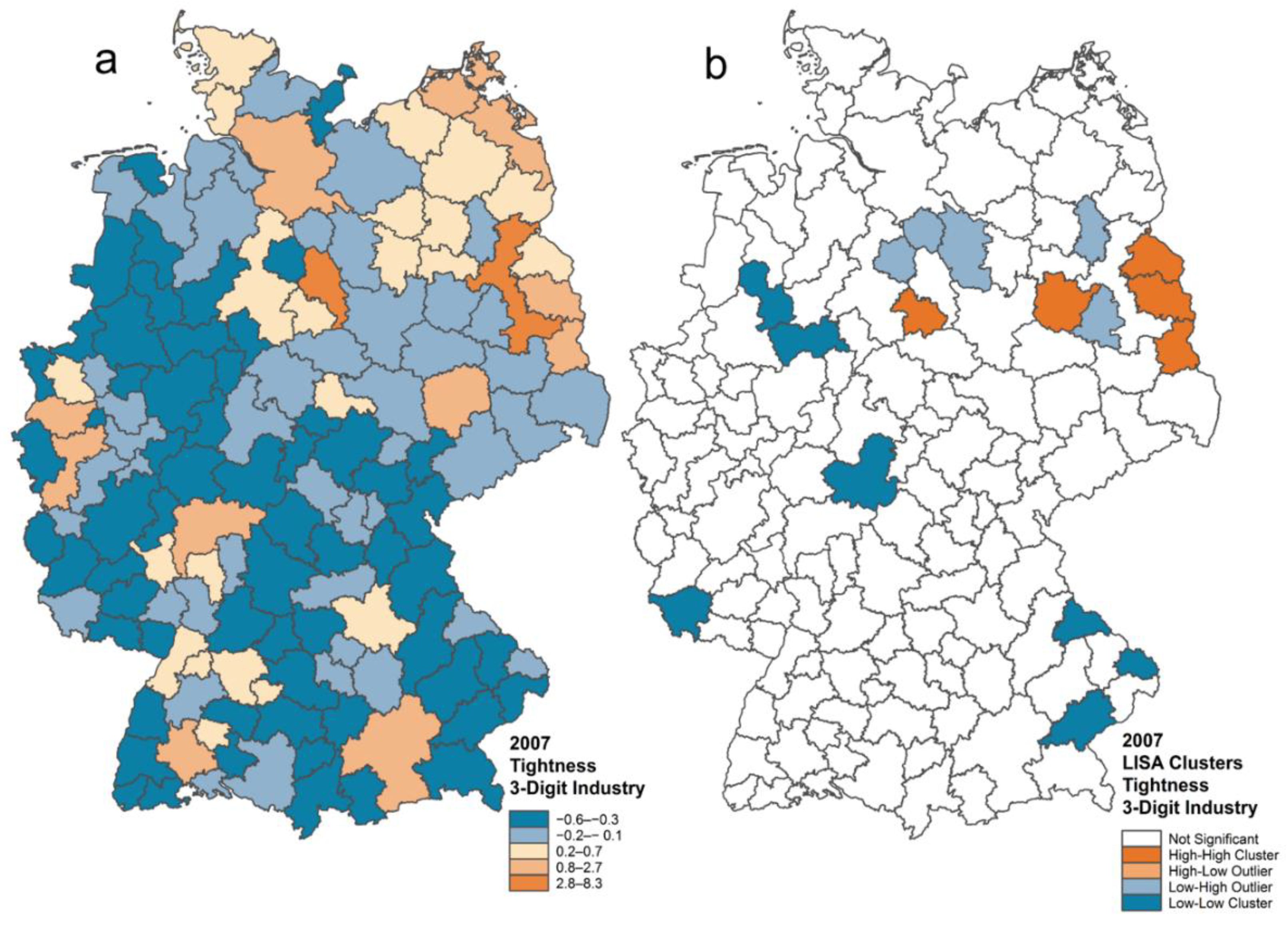
Examining the spatial distribution of 2007 tightness, we find that LMRs with high tightness are more prevalent in the former East (Figure 3a), while LMRs with low tightness are prevalent in the west and south of Germany. To identify statistically significant clusters of LMRs with high and low tightness, we applied Anselin’s local Moran’s I [38,39], a metric of spatial association. Spatial clusters are neighboring regions with tightness values more similar to one another than would be anticipated under spatial randomness. The areas of interest are “high-high” and “low-low”, which are statistically significant spatial clusters of high and low tightness, respectively. Results presented in Figure 3b confirm that a cluster of labor markets with high tightness existed in 2007 in Eastern Germany.
3.5. Tightness, Productivity, and Economic Shocks
Having calculated each area’s tightness under each of the eight empirical treatments, we then correlated those values with the area’s economic performance. We took 2-year change in per capita GDP as our measure of economic performance, calculating it for the periods 2007–2009 and 2009–2011. Correlations for the eight empirical cases are presented in Table 2. In all cases, tightness is negatively correlated with changes in GDP during the shock and positively correlated with changes in GDP during recovery. Furthermore, we find that correlations are stronger when using 3-digit industry aggregations versus 4-digit industry aggregations, and they are stronger when using labor market regions versus counties.
This suggests that LMRs are more functional regarding regional economic attributes than counties. It also suggests that 4-digit industry aggregations may be too sparse to meaningfully inform our metric of connectedness. Thus, we focus our discussion of this work primarily on metrics calculated using LMRs and 3-digit industry data.
Overall, our finding that regions with higher tightness had larger percentage drops in productivity following a shock is consistent with the Panarchy theory of resilience, which asserts that as systems increase in connectedness, they become more brittle and fragile [21]. This finding also concurs with an analogous study of the effects of the 2007–2009 recession on U.S. metropolitan statistical areas [12].
However, the fact that regions with high tightness performed better during the recovery phase should be interpreted with caution. The recovery period following a shock may not be comparable to periods without shocks and so we cannot conclude that tighter economies are, in general, more productive.
3.6. A First Comparison of Tightness Effects and COVID-19 Implications
At first glance, the impact of the COVID-19 pandemic on the German economy was quite comparable to the Great Recession: GDP in 2020 declined by 5.0%, which was similar to its decline in 2009 of 5.6%. But does this correspond with a similar association between tightness and regional economic performance during these two shocks?
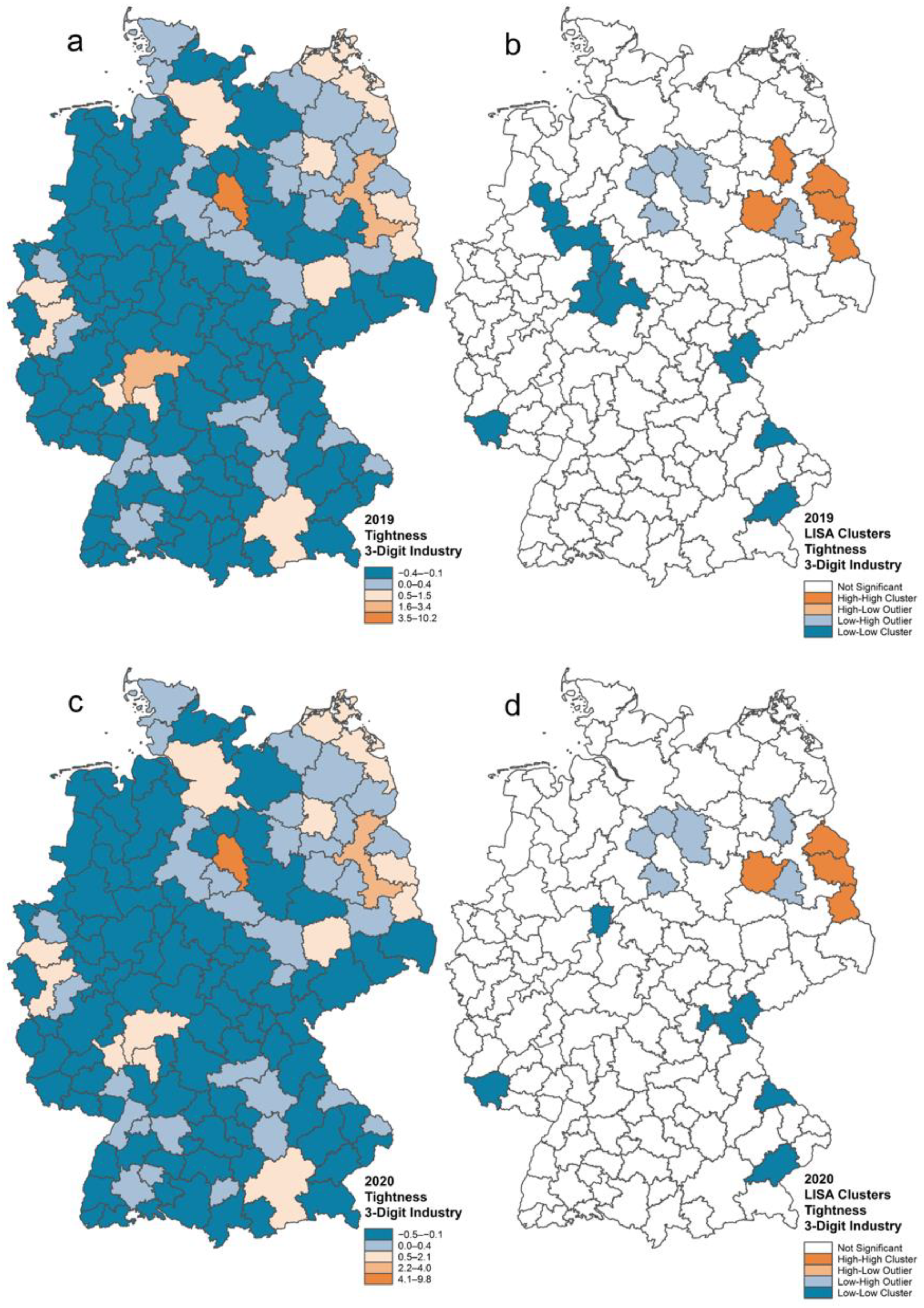
Having demonstrated that tightness in 2007 was correlated with worse performance during the subsequent shock, we calculated tightness during the first months of the COVID-19 pandemic using the latest years of available employment data. The spatial distribution of tightness for 2019 and 2020 is presented in Figure 4.
Our analysis suggests that the effect of the COVID-19 pandemic on regional employment (regional GDP data were not yet available at the time of this study) was very different from the Great Recession. Comparing September to December 2008 employment development with March to June 2020, regional employment declines are distributed more evenly across counties in the COVID 19 crisis than in the Great Recession. Furthermore, short-time work—an instrument of German labor market policy that subsidizes wages for staff that would otherwise have been laid-off due to the economic conditions—varies much more evenly across regions during the pandemic than it did during the Great Recession.
Figure 4 also indicates that tightness during the COVID-19 pandemic was not as negatively correlated with changes in economic performance as during the Great Recession. The crucial factor for this is that the COVID-19 pandemic was more symmetric in terms of sectors being affected significantly negative by the supply shock and contraction of demand, whereas the Great Recession primarily hit export-oriented manufacturing industries and only parts of the services sector (especially financial services). Once more data become available on the regional economic performance during and after the COVID-19 pandemic, our results should be set into a broader perspective to cover the impact of tightness on GDP and employment both during a shock and the recovery.
4. Conclusions
In this study, we used a novel metric to assess the level of internal connectedness of German regions and to assess how that measure relates to economic performance during and after the shock of the Great Recession. Ours is the first study to apply this metric to a country other than the U.S. Like U.S. results, we found that regions with more tightly connected industry structures had larger drops in per capita GDP during the initial shock and larger growth during the recovery. This suggests a tradeoff faced by regional economic policy makers between higher productivity and higher resilience.
However, our study examined a very specific shock in terms of type and scope, and we are careful not to generalize our results to all shocks a region might face. As shown in Section 3.6, pandemics and other biological threats seem to yield—given a specific industry interconnectedness—different economic outcomes, and this caution seems to be justified. For other types of shock, such as trade wars, natural disasters including climate shocks/extreme weather events, or cyber-attacks, our metric of tightness may also suggest different implications for economic performance.
Further research is needed to clarify the role of industry interconnectedness under different types of shock. On a national level, our metric could be used to assess if a certain degree of tightness might increase the resilience or precariousness of supply chains during disruptions, and thus promote economic and national security as well as the capacity to respond to external shocks.
It is also important to note that we analyzed networks of industries. This represents only one dimension of complex regional economies. Others have conducted similar studies using occupations [24,40], skills [13,41], and technologies [42]. Thus, future studies should seek to combine results from these multiple economic dimensions to gain richer insights into the dynamics and resilience of individual countries.
Finally, we recognize that both our metric of tightness and relatedness metrics derived from Frenken et al. [31] have a complex relationship with diversity and that diversity has its own complex relationship with resilience. Future research should seek to disentangle and characterize these related but distinct attributes of regional economic structure.
Author Contributions
Conceptualization and methodology, S.T.S.; all other tasks, S.T.S., H.S., B.A., and K.W. All authors have read and agreed to the published version of the manuscript.
Funding
This research received no external funding.
Institutional Review Board Statement
Not applicable.
Informed Consent Statement
Not applicable.
Data Availability Statement
All data used in this study are publicly available as described in the text.
Acknowledgments
An early version of this paper was posted as a discussion paper (not peer-review) of the German Institute for Employment Research (IAB) at https://doku.iab.de/discussionpapers/2021/dp0721.pdf (accessed on 15 November 2021).
Conflicts of Interest
The authors declare no conflict of interest.
References
- Buhaug, H.; Urdal, H. An urbanization bomb? Population growth and social disorder in cities. Glob. Environ. Chang. 2013, 23, 1–10. [Google Scholar] [CrossRef]
- President’s Council of Advisors on Science and Technology. Technology and the Future of Cities; Executive Office of the President of the United States: Washington, DC, USA, 2016.
- Vandecasteele, I.; Baranzelli, C.; Siragusa, A.; Aurambout, J.P. (Eds.) The Future of Cities–Opportunities, Challenges and the Way Forward; Publications Office of the European Union: Luxembourg, 2019. [Google Scholar]
- Batty, M. Inventing Future Cities; The MIT Press: Cambridge, MA, USA, 2018. [Google Scholar]
- Healy, P. Urban Complexity and Spatial Strategies: Towards a Relational Planning for Our Times; Routledge: London, UK, 2007. [Google Scholar]
- Batty, M. The New Science of Cities; The MIT Press: Cambridge, MA, USA, 2013. [Google Scholar]
- Lobo, J.; Alberti, M.; Allen-Dumas, M.; Arcaute, E.; Barthelemy, M.; Bojorquez Tapia, L.A.; Brail, S.; Bettencourt, L.; Beukes, A.; Chen, W.Q.; et al. Urban Science: Integrated Theory from the First Cities to Sustainable Metropolises. SSRN Electron. J. 2020. [Google Scholar] [CrossRef]
- McPhearson, T.; Haase, D.; Kabisch, N.; Gren, Å. Advancing understanding of the complex nature of urban systems. Ecol. Indic. 2016, 70, 566–573. [Google Scholar] [CrossRef]
- Barthelemy, M. The Structure and Dynamics of Cities: Urban Data Analysis and Theoretical Modeling; Cambridge University Press: Cambridge, UK, 2016. [Google Scholar]
- Neal, Z.P. The Connected City: How Networks Are Shaping the Modern Metropolis; Routledge: New York, NY, USA, 2013. [Google Scholar]
- Shutters, S.T.; Lobo, J.; Strumsky, D.; Muneepeerakul, R.; Mellander, C.; Brachert, M.; Fernandes, T.F.; Bettencourt, L.M.A. The relationship between density and scale in information networks: The case of urban occupational networks. PLoS ONE 2018, 15, e0196915. [Google Scholar] [CrossRef] [Green Version]
- Shutters, S.T.; Muneepeerakul, R.; Lobo, J. Quantifying urban economic resilience through labour force interdependence. Palgrave Commun. 2015, 1, 1–7. [Google Scholar] [CrossRef] [Green Version]
- Shutters, S.T.; Waters, K. Inferring Networks of Interdependent Labor Skills to Illuminate Urban Economic Structure. Entropy 2020, 22, 1078. [Google Scholar] [CrossRef]
- Waters, K.; Shutters, S.T. Industrial structure and a tradeoff between productivity and resilience. SSRN Electron. J. 2020. [Google Scholar] [CrossRef]
- Dustmann, C.; Fitzenberger, B.; Schönberg, U.; Spitz-Oener, A. From Sick Man of Europe to Economic Superstar: Germany’s Resurgent Economy. J. Econ. Perspect. 2014, 28, 167–188. [Google Scholar] [CrossRef] [Green Version]
- Heise, S.; Porzio, T. Spatial Wage Gaps in Frictional Labor Markets; Federal Reserve Bank of Minneapolis: Minneapolis, MN, USA, 2019. [Google Scholar]
- Bade, F.-J.; Alm, B.; Weins, S. Employment Effects of Investment Subsidies by German Regional Policy; ZBW-Leibniz Information Centre for Economics: Hamburg, Germany, 2020. [Google Scholar]
- Otto, A.; Nedelkoska, L.; Neffke, F. Skill-relatedness und Resilienz: Fallbeispiel Saarland. Raumforsch. Raumordn. 2014, 72, 133–151. [Google Scholar] [CrossRef]
- Holling, C.S. Understanding the Complexity of Economic, Ecological, and Social Systems. Ecosystems 2001, 4, 390–405. [Google Scholar] [CrossRef]
- Simmie, J.; Martin, R. The economic resilience of regions: Towards an evolutionary approach. Camb. J. Reg. Econ. Soc. 2010, 3, 27–43. [Google Scholar] [CrossRef] [Green Version]
- Gunderson, L.H.; Holling, C.S. (Eds.) Panarchy: Understanding Transformations in Human and Natural Systems; Island: Washington, DC, USA, 2002. [Google Scholar]
- National Science Foundation Sustainable Urban Systems Subcommittee. Sustainable Urban Systems: Articulating a Long-Term Convergence Research Agenda. A Report from the NSF Advisory Committee for Environmental Research and Education; U.S. National Science Foundation: Washington, DC, USA, 2018.
- Kosfeld, R.; Werner, D.-Ö.A. Deutsche Arbeitsmarktregionen–Neuabgrenzung nach den Kreisgebietsreformen 2007–2011. Raumforsch. Raumordn. 2012, 70, 49–64. [Google Scholar] [CrossRef]
- Muneepeerakul, R.; Lobo, J.; Shutters, S.T.; Gomez-Lievano, A.; Qubbaj, M.R. Urban Economies and Occupation Space: Can They Get “There” from “Here”? PLoS ONE 2013, 8, e73676. [Google Scholar] [CrossRef] [PubMed] [Green Version]
- Liu, G.; Wong, L.; Chua, H.N. Complex discovery from weighted PPI networks. Bioinformatics 2009, 25, 1891–1897. [Google Scholar] [CrossRef] [PubMed]
- Tokuyama, T. Algorithms and Computation. In Proceedings of the 18th International Symposium, ISAAC 2007, Sendai, Japan, 17–19 December2007. [Google Scholar]
- Burda, M.C.; Hunt, J. What Explains the German Labor Market Miracle in the Great Recession? Brook. Pap. Econ. Act. 2011, 42, 273–319. [Google Scholar] [CrossRef] [Green Version]
- Harari, D. Recession and Recovery: The German Experience; UK Parliment, House of Commons Library: London, UK, 2014. [Google Scholar]
- Frenken, K.; Van Oort, F.; Verburg, T. Related Variety, Unrelated Variety and Regional Economic Growth. Reg. Stud. 2007, 41, 685–697. [Google Scholar] [CrossRef] [Green Version]
- Hidalgo, C.A.; Balland, P.-A.; Boschma, R.; Delgado, M.; Feldman, M.; Frenken, K.; Glaeser, E.; He, C.; Kogler, D.F.; Morrison, A.; et al. The Principle of Relatedness. In Research and Innovation Forum 2020; Springer: Singapore, 2018; pp. 451–457. [Google Scholar]
- Content, J.; Frenken, K. Related variety and economic development: A literature review. Eur. Plan. Stud. 2016, 24, 2097–2112. [Google Scholar] [CrossRef]
- Corrigendum. Reg. Stud. 2015, 49, 1938–1940. [CrossRef] [Green Version]
- Essletzbichler, J. Relatedness, Industrial Branching and Technological Cohesion in US Metropolitan Areas. Reg. Stud. 2013, 49, 752–766. [Google Scholar] [CrossRef] [Green Version]
- O’Clery, N.; Heroy, S.; Hulot, F.; Beguerisse-Diaz, M. Unravelling the forces underlying urban industrial agglomeration. arXiv 2019, arXiv:1903.09279v2. [Google Scholar]
- Marshall, A. Principles of Economics; MacMillan: London, UK, 1920. [Google Scholar]
- Ellison, G.; Glaeser, E.L.; Kerr, W.R. What Causes Industry Agglomeration? Evidence from Coagglomeration Patterns. Am. Econ. Rev. 2010, 100, 1195–1213. [Google Scholar] [CrossRef] [Green Version]
- MATLAB. Nonclassical Multidimensional Scaling Using Mdscale; The Mathworks Inc.: Natick, MA, USA, 2020. [Google Scholar]
- Anselin, L. Local Indicators of Spatial Association-LISA. Geogr. Anal. 1995, 27, 93–115. [Google Scholar] [CrossRef]
- Fotheringham, S. Trends in quantitative methods I: Stressing the local. Prog. Hum. Geogr. 1997, 21, 88–96. [Google Scholar] [CrossRef]
- Farinha, T.; Balland, P.-A.; Morrison, A.; Boschma, R. What drives the geography of jobs in the US? Unpacking relatedness. Ind. Innov. 2019, 26, 988–1022. [Google Scholar] [CrossRef] [Green Version]
- Alabdulkareem, A.; Frank, M.R.; Sun, L.; AlShebli, B.; Hidalgo, C.; Rahwan, I. Unpacking the polarization of workplace skills. Sci. Adv. 2018, 4, eaao6030. [Google Scholar] [CrossRef] [Green Version]
- Kogler, D.F.; Rigby, D.L.; Tucker, I. Mapping Knowledge Space and Technological Relatedness in US Cities. Eur. Plan. Stud. 2013, 21, 1374–1391. [Google Scholar] [CrossRef]
Figure 1.
Constructing the 2007 German industry interdependence network. Industries that tend to co-occur together in regions have x > 0 and will tend to be closer to each other in the final network. Industries that rarely occur together will have x~0 or x < 0 and will be pushed apart in the final network. Combining all network pairs results in the final German industry network (left). Each node represents a 3-digit industry and, while the placement of nodes is generally arbitrary, the distance between any two nodes is a function of an industry’s interdependence x with all other industries. Links between nodes have been removed for visual clarity.

Figure 2.
Comparison of two German labor market regions (LMRs). The subnetworks locations of Hamburg and Weißenburg-Gunzenhausen are shown within the 2007 German industry network of Figure 1. Qualitatively, the density of Hamburg nodes is higher than those of Weißenburg-Gunzenhausen. We quantify this visually intuitive difference in a regional tightness metric T. Links have been removed for clarity.

Figure 3.
Spatial distribution and autocorrelation of LMR tightness values, 2007. (a) Tightness and (b) Anselin’s local Moran’s I (LISA) shown here were calculated at the 3-digit industry code level. Clusters shown in (b) are significant at a confidence level of 0.05 using k-nearest neighbors = 4.
Figure 3.
Spatial distribution and autocorrelation of LMR tightness values, 2007. (a) Tightness and (b) Anselin’s local Moran’s I (LISA) shown here were calculated at the 3-digit industry code level. Clusters shown in (b) are significant at a confidence level of 0.05 using k-nearest neighbors = 4.

Figure 4.
Current spatial distribution and autocorrelation of LMR tightness values, 2019 and 2020. Tightness (a,c) and Anselin’s local Moran’s I (LISA) (b,d) were calculated at the 3-digit industry code level. Clusters shown in (b) are significant at a confidence level of 0.05 using k-nearest neighbors = 4. Between 2007 and 2019 the cluster of high-high tightness areas in Eastern Germany grew in size, while the clusters of low-low tightness in central Germany also grew. Thus, the most recent employment data indicate a growing spatial segregation within Germany in terms of economic tightness.


Table 1.
Highest and lowest ranked labor market regions based on 2007 tightness values T.
| Rank | Labor Market Region (LMR) | T1 |
|---|---|---|
| 1 | Wolfsburg (007) | 8.27 |
| 2 | Berlin (109) | 5.10 |
| 3 | Frankfurt am Main (043) | 2.68 |
| 4 | Frankfurt an der Oder (110) | 2.05 |
| 5 | Cottbus (118) | 1.68 |
| 137 | Trier (054) | −0.61 |
| 138 | Koblenz (049) | −0.61 |
| 139 | Kleve (027) | −0.62 |
| 140 | Minden (036) | −0.64 |
| 141 | Passau (086) | −0.64 |
1 T presented as the normalized z-score of raw tightness values.
Table 2.
Correlation coefficients between an area’s tightness T in 2007 and 2009 and the area’s change in GDP per worker over the subsequent two years. Correlations are presented for two types of spatial units and for both 3-digit and 4-digit industry levels of employment aggregation.
Table 2.
Correlation coefficients between an area’s tightness T in 2007 and 2009 and the area’s change in GDP per worker over the subsequent two years. Correlations are presented for two types of spatial units and for both 3-digit and 4-digit industry levels of employment aggregation.
| Labor Market Regions (N = 141) | Counties (N = 401) | |||
|---|---|---|---|---|
| Industry Level | 3-digit | 4-digit | 3-digit | 4-digit |
| T (2007) vs. GDP change, 2007–2009 | −0.22 ** | −0.19 * | −0.20 *** | −0.09 n/s |
| T (2009) vs. GDP change, 2009–2011 | 0.34 *** | 0.25 ** | 0.27 *** | 0.14 ** |
* significant at p < 0.05; ** significant at p < 0.01; *** significant at p < 0.001; n/s = not significant.
Publisher’s Note: MDPI stays neutral with regard to jurisdictional claims in published maps and institutional affiliations. |
© 2021 by the authors. Licensee MDPI, Basel, Switzerland. This article is an open access article distributed under the terms and conditions of the Creative Commons Attribution (CC BY) license (https://creativecommons.org/licenses/by/4.0/).
Share and Cite
MDPI and ACS Style
Shutters, S.T.; Seibert, H.; Alm, B.; Waters, K. Industry Interconnectedness and Regional Economic Growth in Germany. Urban Sci. 2022, 6, 1. https://0-doi-org.brum.beds.ac.uk/10.3390/urbansci6010001
AMA Style
Shutters ST, Seibert H, Alm B, Waters K. Industry Interconnectedness and Regional Economic Growth in Germany. Urban Science. 2022; 6(1):1. https://0-doi-org.brum.beds.ac.uk/10.3390/urbansci6010001
Chicago/Turabian StyleShutters, Shade T., Holger Seibert, Bastian Alm, and Keith Waters. 2022. "Industry Interconnectedness and Regional Economic Growth in Germany" Urban Science 6, no. 1: 1. https://0-doi-org.brum.beds.ac.uk/10.3390/urbansci6010001