
A Case Study Evaluating Water Quality and Reach-, Buffer-, and Watershed-Scale Explanatory Variables of an Urban Coastal Watershed

Abstract
:1. Introduction
2. Materials and Methods
2.1. Field-Area Description
2.2. Study Design
2.3. 2012 Water Quality Monitoring
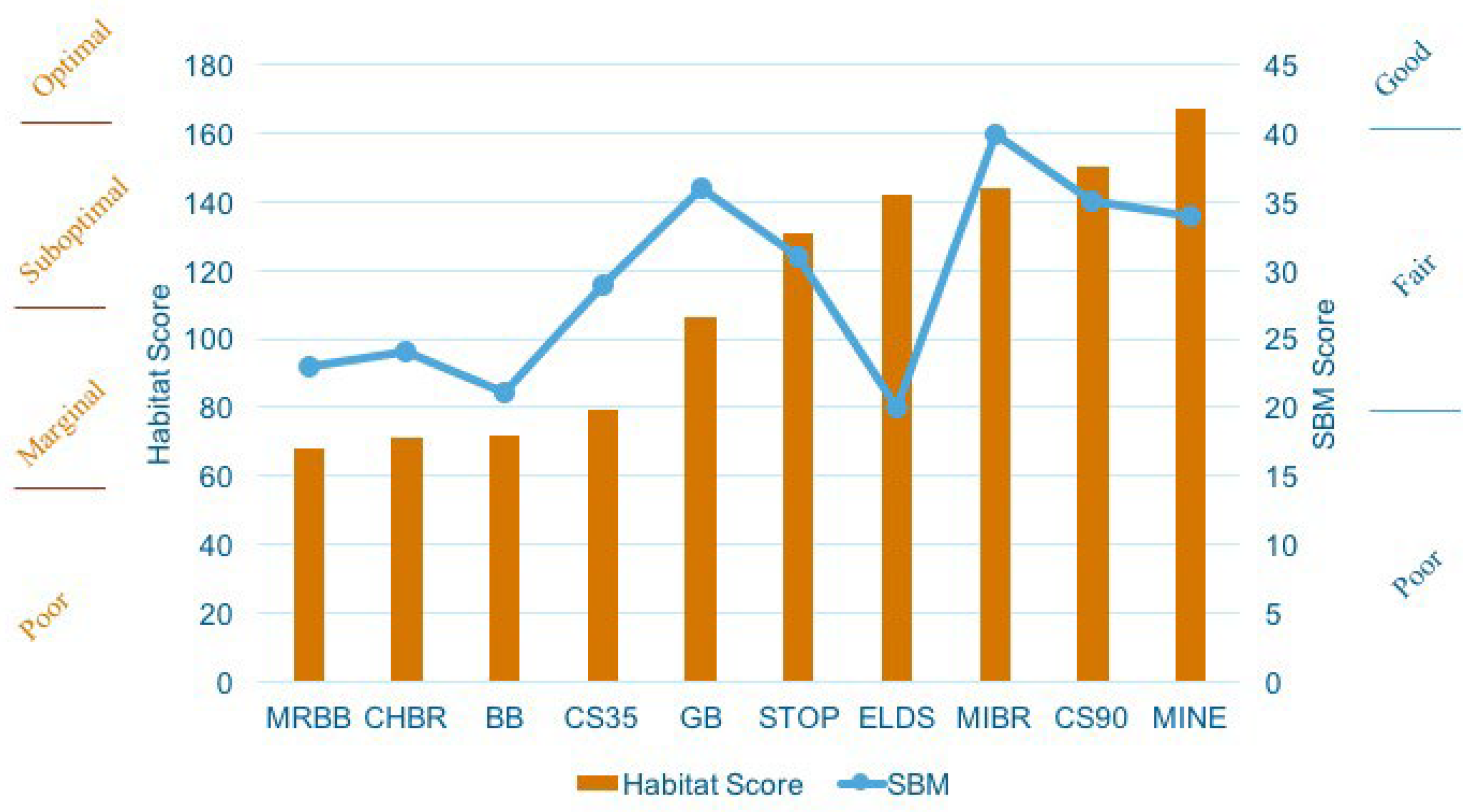
2.3.1. Reach-Scale Habitat Quality
2.3.2. Physical-Chemical Analyses
2.3.3. Macroinvertebrate Sampling and Analysis
2.4. Sub-Watershed and Local Buffer GIS Data Collection
2.5. Data Analysis
2.5.1. Data Reduction
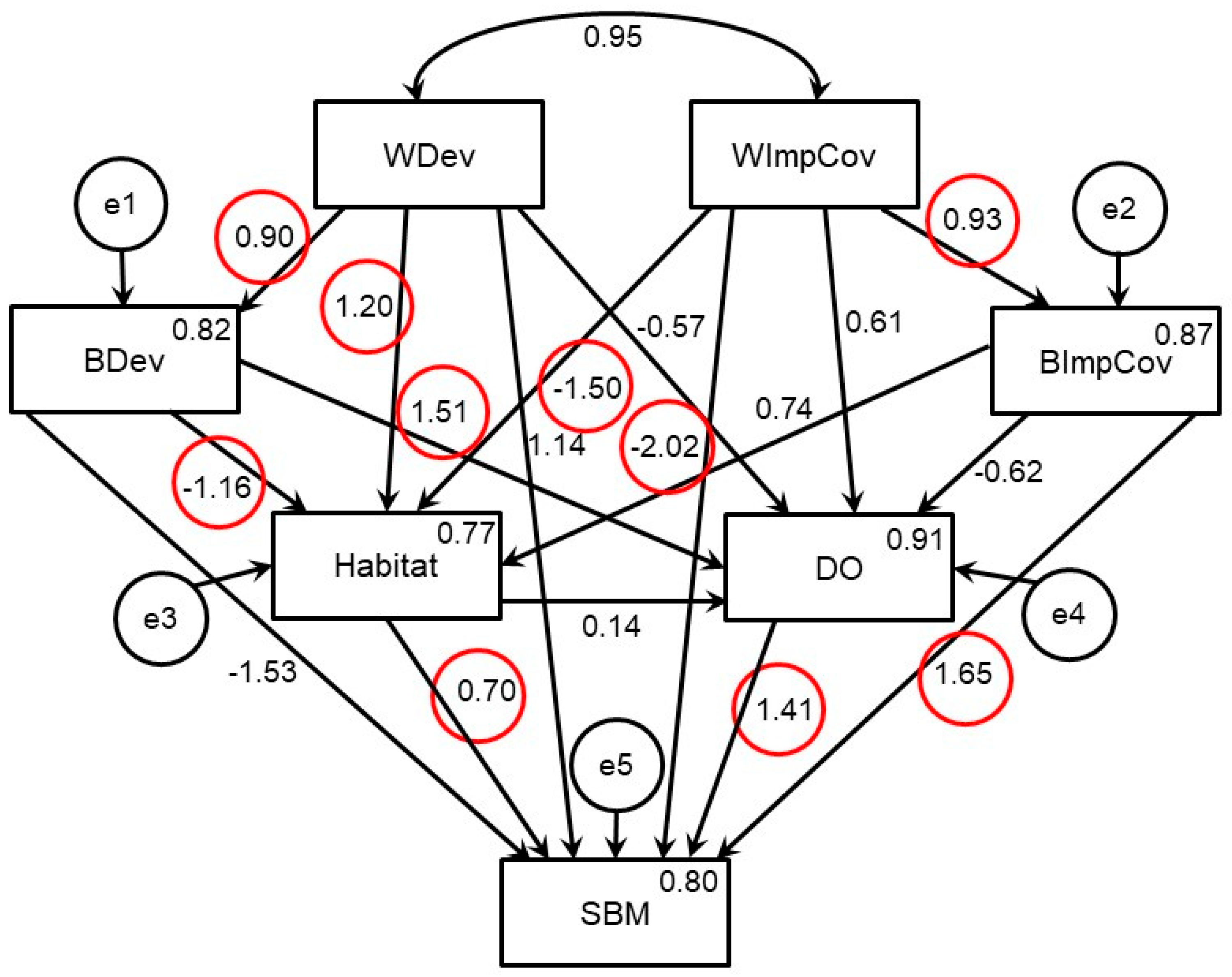
2.5.2. Path Analysis
3. Results
3.1. Water Quality
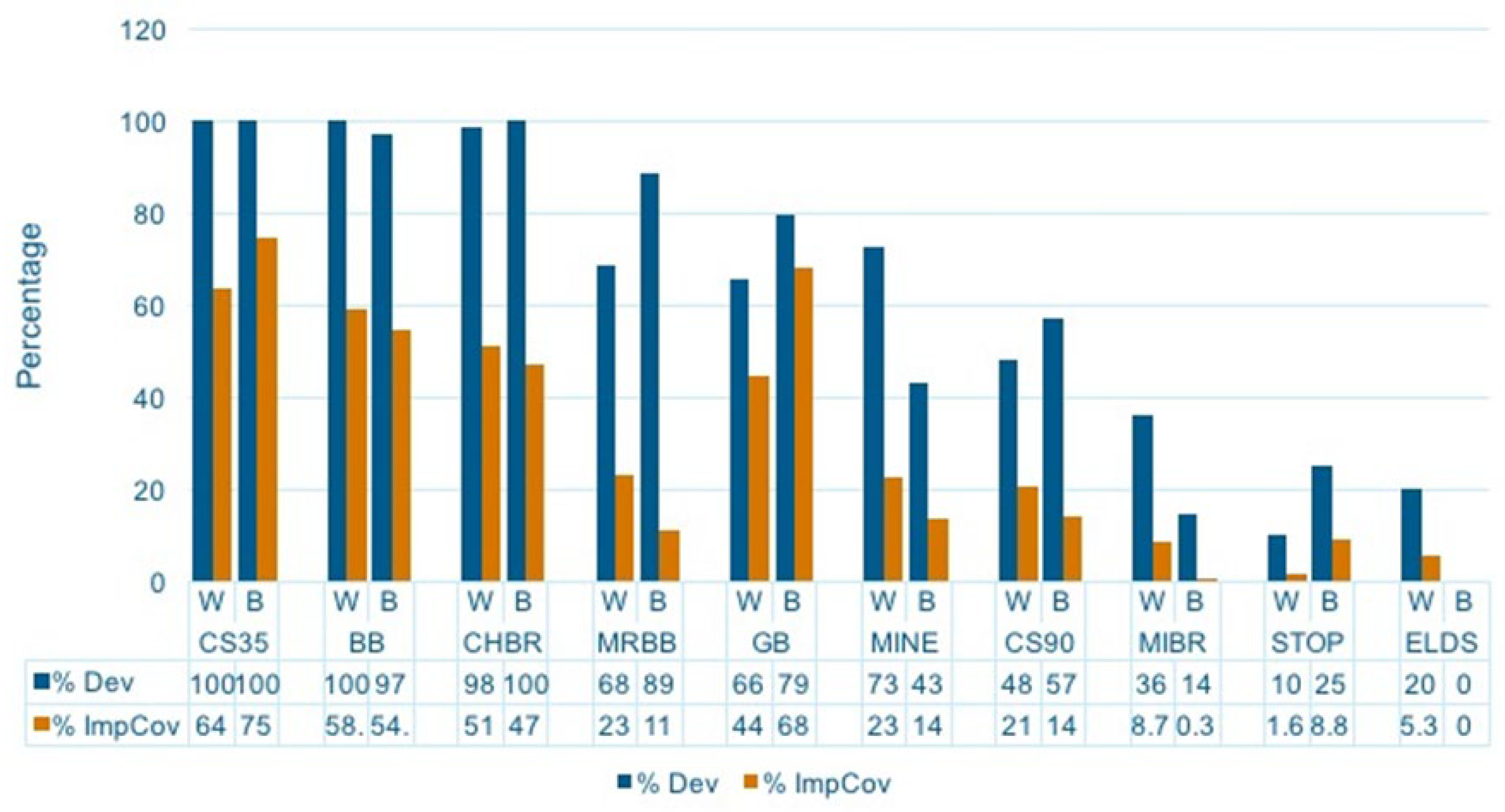
3.2. GIS Analysis
3.3. Path Analysis
4. Discussion
4.1. Overview
4.2. Water Quality
4.3. Path Analysis
4.3.1. Impervious Cover
4.3.2. Habitat and DO Positive Direct Effects on SBM
4.3.3. Development Not Significantly Directly Effecting SBM
4.3.4. BDev Significant Indirect Effect on SBM
4.3.5. Path Analysis Summary
5. Conclusions
Author Contributions
Funding
Institutional Review Board Statement
Informed Consent Statement
Data Availability Statement
Acknowledgments
Conflicts of Interest
References
- Frissell, C.A.; Liss, W.J.; Warren, C.E.; Hurley, M.D. A Hierarchical Framework for Stream Habitat Classification: Viewing Streams in a Watershed Context. Environ. Manag. 1986, 10, 199–214. [Google Scholar] [CrossRef]
- Maddock, I.; Harby, A.; Kemp, P.; Wood, P.J. Ecohydraulics: An Integrated Approach; John Wiley & Sons: Hoboken, NJ, USA, 2013. [Google Scholar]
- Wiens, J.A. Riverine Landscapes: Taking Landscapes Ecology into the Water. Freshw. Biol. 2002, 47, 501–515. [Google Scholar] [CrossRef]
- Allan, J.D. Landscapes and Riverscapes: The Influence of Land Use on Stream Ecosystems. Annu. Rev. Ecol. Evol. Syst. 2004, 35, 257–284. [Google Scholar] [CrossRef] [Green Version]
- Walsh, C.J.; Roy, A.H.; Feminella, J.W.; Cottingham, P.D.; Groffman, P.M.; Morgan, R.P. The Urban Stream Syndrome: Current Knowledge and the Search for a Cure. J. N. Am. Benthol. Soc. 2005, 24, 706–723. [Google Scholar] [CrossRef]
- Roy, A.H.; Capps, K.A.; El-Sabaawi, R.W.; Jones, K.L.; Parr, T.B.; Ramírez, A.; Smith, R.F.; Walsh, C.J.; Wenger, S.J. Urbanization and Stream Ecology: Diverse Mechanisms of Change. Freshw. Sci. 2016, 35, 272–277. [Google Scholar] [CrossRef] [Green Version]
- Booth, D.B.; Roy, A.H.; Smith, B.; Capps, K.A. Global Perspectives on the Urban Stream Syndrome. Freshw. Sci. 2016, 35, 412–420. [Google Scholar] [CrossRef] [Green Version]
- Maloney, K.O.; Weller, D.E. Anthropogenic Disturbance and Streams: Land Use and Land-use Change Affect Stream Ecosystems via Multiple Pathways. Freshw. Biol. 2011, 56, 611–626. [Google Scholar] [CrossRef]
- Barbour, M.T.; Gerritsen, J.; Snyder, B.D.; Stribling, J.B. Rapid Bioassessment Protocols for Use in Streams and Wadeable Rivers: Periphyton, Benthic Macroinvertebrates, and Fish, 2nd ed.; EPA 841-B-99-002; U.S. Environmental Protection Agency, Office of Water: Washington, DC, USA, 1999.
- Alberts, J.M.; Fritz, K.M.; Buffam, I. Response to Basal Resources by Stream Macroinvertebrates Is Shaped by Watershed Urbanization, Riparian Canopy Cover, and Season. Freshw. Sci. 2018, 37, 640–652. [Google Scholar] [CrossRef]
- United States Environmental Protection Agency. Volunteer Stream Monitoring: A Methods Manual; 4503F EPA 841-B-97-003; Office of Water, Environmental Protection Agency: Washington, DC, USA, 1997; p. 227.
- Arnold, C.L., Jr.; Gibbons, C.J. Impervious Surface Coverage: The Emergence of a Key Environmental Indicator. J. Am. Plan. Assoc. 1996, 62, 243–258. [Google Scholar] [CrossRef]
- Li, Z.; Peng, L.; Wu, F. The Impacts of Impervious Surface on Water Quality in the Urban Agglomerations of Middle and Lower Reaches of the Yangtze River Economic Belt From Remotely Sensed Data. IEEE J. Sel. Top. Appl. Earth Obs. Remote Sens. 2021, 14, 8398–8406. [Google Scholar] [CrossRef]
- Li, L.; Yu, Q.; Gao, L.; Yu, B.; Lu, Z. The Effect of Urban Land-Use Change on Runoff Water Quality: A Case Study in Hangzhou City. Int. J. Environ. Res. Public Health 2021, 18, 10748. [Google Scholar] [CrossRef] [PubMed]
- Kim, D.-K.; Jo, H.; Park, K.; Kwak, I.-S. Assessing Spatial Distribution of Benthic Macroinvertebrate Communities Associated with Surrounding Land Cover and Water Quality. Appl. Sci. 2019, 9, 5162. [Google Scholar] [CrossRef] [Green Version]
- Sliva, L.; Williams, D.D. Buffer Zone versus Whole Catchment Approaches to Studying Land Use Impact on River Water Quality. Water Res. 2001, 35, 3462–3472. [Google Scholar] [CrossRef]
- King, R.S.; Baker, M.E.; Whigham, D.F.; Weller, D.E.; Jordan, T.E.; Kazyak, P.F.; Hurd, M.K. Spatial Considerations for Linking Watershed Land Cover to Ecological Indicators in Streams. Ecol. Appl. 2005, 15, 137–153. [Google Scholar] [CrossRef] [Green Version]
- Akintunde, A. Path Analysis Step by Step Using Excel. J. Tech. Sci. Technol. 2012, 1, 9–15. [Google Scholar]
- Pedhazur, E.; Kerlinger, F. Multiple Regression in Behavioral Research: Explanation and Prediction, 2nd ed.; Holt, Rinehart, and Winston: New York, NY, USA, 1982. [Google Scholar]
- Ciarfella, C.E. Efficacy of Citizen Science in Water Quality Studies: A Macroinvertebrate Biomonitoring Project in the Charles River Watershed, Massachusetts. Master’s Thesis, University of Massachusetts Boston, Boston, MA, USA, 2014. [Google Scholar]
- Charles River Watershed Association. Charles River Watershed Association. Available online: http://www.crwa.org/charles-river-watershed (accessed on 28 May 2017).
- Myette, C.F.; Simcox, A.C. Water Resources and Aquifer Yields in the Charles River Basin, Massachusetts; US Department of the Interior, US Geological Survey: Denver, CO, USA, 1992; Volume 88.
- Weiskel, P.K. The Charles River, Eastern Massachusetts: Scientific Information in Support of Environmental Restoration; Report 47; US Geological Survey: Denver, CO, USA, 2007.
- U.S. Department of Interior. StreamStats Version 3.0. Available online: http://streamstatsags.cr.usgs.gov/v3_beta/BCreport.htm (accessed on 6 December 2016).
- Yentsch, C.S.; Menzel, D.W. A Method for the Determination of Phytoplankton Chlorophyll and Phaeophytin by Fluorescence. In Deep Sea Research and Oceanographic Abstracts; Oceanographic Abstracts; Elsevier Science: Amsterdam, The Netherlands, 1963; Volume 10, pp. 221–231. [Google Scholar]
- Greenberg, A.E.; Clesceri, L.S.; Eaton, A.D.; Franson, M.A.H. Standard Methods for the Examination of Water and Wastewater, 18th ed.; American Public Health Administration, American Water Works Association and Water Environment Federation: Washington, DC, USA, 1992. [Google Scholar]
- Crumpton, W.G.; Isenhart, T.M.; Mitchell, P.D. Nitrate and Organic N Analysis with Second-Derivative Spectroscopy. Limnol. Oceanogr. 1992, 37, 907–913. [Google Scholar] [CrossRef] [Green Version]
- Merritt, R.W.; Cummins, K.W.; Berg, M.B. An Introduction to the Aquatic Insects of North America, 4th Edn. Kendall; Hunt Publishing Company: Dubuque, IA, USA, 2008. [Google Scholar]
- Thorp, J.H.; Covich, A.P. Ecology and Classification of North American Freshwater Invertebrates; Academic Press: Cambridge, MA, USA, 2009. [Google Scholar]
- Komínková, D. The Urban Stream Syndrome—A Mini-Review. Open Environ. Biol. Monit. J. 2012, 5, 24–29. [Google Scholar] [CrossRef] [Green Version]
- Henderson, N.D. The Effects of Global Change Drivers on Water Quality in an Urban Northeastern Coastal Ecoregion. Ph.D. Thesis, University of Massachusetts Boston, Boston, MA, USA, 2018. [Google Scholar]
- Schiff, R.; Benoit, G. Effects of Impervious Cover at Multiple Spatial Scales on Coastal Watershed Streams 1. JAWRA J. Am. Water Resour. Assoc. 2007, 43, 712–730. [Google Scholar] [CrossRef]
- Zarriello, P.J.; Barlow, L.K. Measured and Simulated Runoff to the Lower Charles River, Massachusetts, October 1999-September 2000; US Department of the Interior, US Geological Survey: Denver, CO, USA, 2002.
- O’connor, N.A. The Effects of Habitat Complexity on the Macroinvertebrates Colonising Wood Substrates in a Lowland Stream. Oecologia 1991, 85, 504–512. [Google Scholar] [CrossRef]
- Kaller, M.D.; Kelso, W.E. Association of Macroinvertebrate Assemblages with Dissolved Oxygen Concentration and Wood Surface Area in Selected Subtropical Streams of the Southeastern USA. Aquat. Ecol. 2007, 41, 95–110. [Google Scholar] [CrossRef]
- Pearl, J. Comment: Understanding Simpson’s Paradox. Am. Stat. 2014, 68, 8–13. [Google Scholar] [CrossRef]
- Pander, J.; Geist, J. Ecological Indicators for Stream Restoration Success. Ecol. Indic. 2013, 30, 106–118. [Google Scholar] [CrossRef]


| River | Station ID | Town | Coordinates (Lat./Lon.) | Predominant Land Use |
|---|---|---|---|---|
| Beaver Brook | BB | Waltham | 42.38099 –71.21727 | Residential |
| Charles River | CS35 | Milford | 42.13970 –71.51253 | Urban |
| Charles River | ELDS | Milford | 42.18350 –71.51222 | Forests |
| Charles River | CS90 | Bellingham | 42.09435 –71.47668 | Forests |
| Cheesecake Brook | CHBR | Newton | 42.35609 –71.21499 | Residential/ Recreational |
| Godfrey Brook | GB | Milford | 42.12954 –71.51854 | Urban |
| Mine Brook | MINE | Franklin | 42.12469 –71.43083 | Forests/ Wetlands |
| Miscoe Brook | MIBR | Franklin | 42.04090 –71.42646 | Forests |
| Muddy River Babbling Brook | MRBB | Brookline | 42.32431 –71.11639 | Forests/ Recreational |
| Stop River | STOP | Medfield | 42.17221 –71.31730 | Wetlands |
| Station | pH | Temp (°C) | DO (% sat) | SpC (µS/ cm) | Sal. (ppt) | Chl_a (mg/ L) | TDS (mg/ L) | NVSS (mg/ L) | TSS (mg/ L) |
|---|---|---|---|---|---|---|---|---|---|
| BB | 7.64 | 10.5 | 69.9 | 548 | 0.4 | BDL | 494.0 | 0.0 * | 1.7 |
| 35CS | 8.75 | 18.9 | 92.9 | 536 | 0.3 | BDL | 396.5 | 0.4 | 3.0 |
| 90CS | 8.55 | 18.4 | 74.4 | 618 | 0.3 | 0.0 * | 403.0 | 0.0 * | 1.4 |
| ELDS | 5.88 | 10.5 | 8.3 | 134.5 | 0.1 | BDL | 87.1 | 0.0 * | 0.0 * |
| CHBR | 7.66 | 14.8 | 95.8 | 817 | 0.4 | 0.0 * | 533.0 | 0.0 * | 1.1 |
| GB | 9.14 | 15 | 75.1 | 120.4 | 0.1 | BDL | 76.1 | 0.0 * | 2.3 |
| MINE | 8.25 | 14.5 | 40.6 | 490.9 | 0.2 | 0.0 * | 318.5 | 16.6 | 29.0 |
| MIBR | 7.75 | 11 | 39.6 | 293.8 | 0.1 | BDL | 191.1 | 6.4 | 28.6 |
| MRBB | 8.51 | 11.1 | 91.9 | 370 | 0.3 | BDL | 341.9 | 0.0 * | 2.0 |
| STOP | 0.03 ** | 16.4 | 36.1 | 364.7 | 0.2 | 0.0 * | 237.3 | 21.9 | 34.6 |
| Station | N:P | NO3+ (mol/L) | NO2+ (mol/L) | PO4+ (mol/L) | NH3− (mol/L) |
|---|---|---|---|---|---|
| BB | 150.85 | 65.79 | 0.03 | 0.56 | 18.07 |
| 35CS | 335.77 | 40.57 | 0.00 | 0.14 | 4.83 |
| 90CS | 1659.08 | 252.13 | 0.18 | 0.16 | 8.84 |
| ELDS | 49.54 | 5.48 | 0.02 | 0.19 | 3.70 |
| CHBR | 203.42 | 221.89 | 0.01 | 1.10 | 2.58 |
| GB | 1206.34 | 127.21 | BDL | 0.11 | 7.23 |
| MINE | 16.48 | 1.48 | BDL | 0.20 | 1.77 |
| MIBR | 273.45 | 36.59 | 0.20 | 0.14 | 2.71 |
| MRBB | 51.12 | 13.04 | 0.00 | 0.31 | 2.72 |
| STOP | 122.76 | 68.58 | 0.05 | 0.67 | 13.22 |
| Station | Sub-Watershed | % Area | Buffer | % Area |
|---|---|---|---|---|
| BB | Developed | 100.0 | Developed | 97.1 |
| Undeveloped | 0.0 | Undeveloped | 2.9 | |
| Impervious | 58.8 | Impervious | 54.7 | |
| 35CS | Developed | 100.0 | Developed | 100.0 |
| Undeveloped | 0.0 | Undeveloped | 0.0 | |
| Impervious | 63.5 | Impervious | 74.5 | |
| 90CS | Developed | 47.8 | Developed | 57.1 |
| Undeveloped | 50.7 | Undeveloped | 42.9 | |
| Impervious | 20.7 | Impervious | 14.0 | |
| ELDS | Developed | 20.2 | Developed | 0.0 |
| Undeveloped | 71.2 | Undeveloped | 100.0 | |
| Impervious | 5.3 | Impervious | 0.0 | |
| CHBR | Developed | 98.3 | Developed | 100.0 |
| Undeveloped | 1.7 | Undeveloped | 0.0 | |
| Impervious | 50.9 | Impervious | 46.9 | |
| GB | Developed | 65.6 | Developed | 79.4 |
| Undeveloped | 11.4 | Undeveloped | 0.0 | |
| Impervious | 44.3 | Impervious | 67.9 | |
| MINE | Developed | 72.7 | Developed | 42.9 |
| Undeveloped | 27.3 | Undeveloped | 57.1 | |
| Impervious | 22.6 | Impervious | 13.7 | |
| MIBR | Developed | 36.0 | Developed | 14.3 |
| Undeveloped | 60.8 | Undeveloped | 85.8 | |
| Impervious | 8.7 | Impervious | 0.3 | |
| MRBB | Developed | 68.3 | Developed | 88.6 |
| Undeveloped | 22.7 | Undeveloped | 11.4 | |
| Impervious | 23.0 | Impervious | 11.1 | |
| STOP | Developed | 10 | Developed | 25.0 |
| Undeveloped | 90 | Undeveloped | 75.0 | |
| Impervious | 1.6 | Impervious | 8.8 |
| Standardized Effects | p-Value | |
|---|---|---|
| WDev > SBM | ||
| Direct Effect | 1.14 | 0.090 |
| Indirect Effect | −0.14 | |
| Total Effect | 1.01 | |
| BDev > SBM | ||
| Direct Effect | −1.53 | 0.070 |
| Indirect Effect | 1.09 | |
| Total Effect | −0.45 | |
| WImpCov > SBM | ||
| Direct Effect | −2.02 | 0.008 * |
| Indirect Effect | 0.86 | |
| Total Effect | −1.16 | |
| BImpCov > SBM | ||
| Direct Effect | 1.65 | 0.002 * |
| Indirect Effect | −0.20 | |
| Total Effect | 1.45 | |
| Habitat > SBM | ||
| Direct Effect | 0.70 | 0.017 * |
| Indirect Effect | 0.20 | |
| Total Effect | 0.90 | |
| DO > SBM | ||
| Direct Effect | 1.41 | 0.002 * |
| Total Effect | 1.41 |
| WImpCov | WDev | BDev | BImpCov | Habitat | DO | |
|---|---|---|---|---|---|---|
| BDev | 0.000 | 0.000 | 0.000 | 0.000 | 0.000 | 0.000 |
| BImpCov | 0.000 | 0.000 | 0.000 | 0.000 | 0.000 | 0.000 |
| Habitat | 0.694 | −1.048 | 0.000 | 0.000 | 0.000 | 0.000 |
| DO | −0.688 | 1.385 | −0.162 | 0.104 | 0.000 | 0.000 |
| SBM | 0.859 | −0.138 | 1.085 | −0.202 | 0.196 | 0.000 |
Publisher’s Note: MDPI stays neutral with regard to jurisdictional claims in published maps and institutional affiliations. |
© 2022 by the authors. Licensee MDPI, Basel, Switzerland. This article is an open access article distributed under the terms and conditions of the Creative Commons Attribution (CC BY) license (https://creativecommons.org/licenses/by/4.0/).
Share and Cite
Heidkamp, L.C.; Christian, A.D. A Case Study Evaluating Water Quality and Reach-, Buffer-, and Watershed-Scale Explanatory Variables of an Urban Coastal Watershed. Urban Sci. 2022, 6, 17. https://0-doi-org.brum.beds.ac.uk/10.3390/urbansci6010017
Heidkamp LC, Christian AD. A Case Study Evaluating Water Quality and Reach-, Buffer-, and Watershed-Scale Explanatory Variables of an Urban Coastal Watershed. Urban Science. 2022; 6(1):17. https://0-doi-org.brum.beds.ac.uk/10.3390/urbansci6010017
Chicago/Turabian StyleHeidkamp, Laurissa C., and Alan D. Christian. 2022. "A Case Study Evaluating Water Quality and Reach-, Buffer-, and Watershed-Scale Explanatory Variables of an Urban Coastal Watershed" Urban Science 6, no. 1: 17. https://0-doi-org.brum.beds.ac.uk/10.3390/urbansci6010017