Article

Brain Melody Interaction: Understanding Effects of Music on Cerebral Hemodynamic Responses

1
School of Computing, The Australian National University, Canberra, ACT 2601, Australia
2
The Australian e-Health Research Centre, Commonwealth Scientific and Industrial Research Organisation, Sydney, NSW 2145, Australia
3
Optus-Curtin Centre of Excellence in AI, Curtin University, Perth, WA 6102, Australia
*
Author to whom correspondence should be addressed.
Multimodal Technol. Interact. 2022, 6(5), 35; https://0-doi-org.brum.beds.ac.uk/10.3390/mti6050035
Submission received: 20 February 2022 / Revised: 19 April 2022 / Accepted: 29 April 2022 / Published: 4 May 2022
(This article belongs to the Special Issue Musical Interactions (Volume II))

Abstract

:
Music elicits strong emotional reactions in people, regardless of their gender, age or cultural background. Understanding the effects of music on brain activity can enhance existing music therapy techniques and lead to improvements in various medical and affective computing research. We explore the effects of three different music genres on people’s cerebral hemodynamic responses. Functional near-infrared spectroscopy (fNIRS) signals were collected from 27 participants while they listened to 12 different pieces of music. The signals were pre-processed to reflect oxyhemoglobin (HbO2) and deoxyhemoglobin (HbR) concentrations in the brain. K-nearest neighbor (KNN), random forest (RF) and a one-dimensional (1D) convolutional neural network (CNN) were used to classify the signals using music genre and subjective responses provided by the participants as labels. Results from this study show that the highest accuracy in distinguishing three music genres was achieved by deep learning models (73.4% accuracy in music genre classification and 80.5% accuracy when predicting participants’ subjective rating of emotional content of music). This study validates a strong motivation for using fNIRS signals to detect people’s emotional state while listening to music. It could also be beneficial in giving personalised music recommendations based on people’s brain activity to improve their emotional well-being.

1. Introduction

A famous line penned by Stevie Wonder in his song “Sir Duke” is “Music is a world within itself, with a language we all understand”. Music is an art form enjoyed and understood by people all around the world. It tends to elicit a variety of emotions in people, which can be reflected in their conscious and unconscious responses. The correlation between music and emotion is often mysterious and thought provoking. Different types of reactions have been reported in regards to people’s reaction to music. Some of them include frustration when a particular style of music is played at a shop, sadness in response to a late-night movie soundtrack, and nostalgia evoked by a familiar song playing on the radio [1]. Music has benefits including increased focus [2], reduction in stress and anxiety levels [3,4], and improvement in memory [5]. Thus, music has a significant impact on our daily life and activities. Music stimuli are also used in therapeutic interventions and have been shown to improve sleep quality [6]. Due to the diverse effects and applications of music, music is frequently used as stimuli in medical and affective computing-related research studies.
Studies in the field of affective computing aim to build computing systems that can accurately understand human emotions. Understanding emotional reactions to music could be beneficial for giving personal music recommendations, which could improve emotional well-being by avoiding inappropriate music. There are different ways to capture data about people’s emotional reactions. The most common methods are self-reports [7,8,9] and facial expressions [10,11,12]. Some other common measures are speech [13], pupillary response [14], and hand and body gestures [15]. However, some of these methods can be prone to high individual biases. For instance, people can sometimes hide their true emotions in their facial expression. Capturing emotional responses using physiological signals is beneficial in such cases as these signals are involuntary and cannot be readily hidden, muted or faked. Studies have also shown that music can induce universal psycho-physiological responses among different groups of people [16]. There are different physiological signals which reflect human emotions. Some of them are electroencephalography (EEG), galvanic skin response (GSR, also known as skin conductance), blood volume pulse (BVP), heart rate (HR), skin temperature (ST) and functional near-infrared spectroscopy (fNIRS). Experiments have demonstrated that music induces specific patterns in the autonomic nervous system (ANS) that reflects a relaxing or arousing state [17]. A significant increase in skin conductance was observed in subjects listening to emotionally intense music [18] and music evoking fear or happiness [19]. Skin temperature can also be influenced by listening to music that induces positive emotions [20]. With the advent of modern wearable technologies, collecting physiological signals is becoming easier day by day.
Activities related to music such as listening to songs and playing an instrument have a strong influence on people’s brain activity [21], and compared to other stimuli, music stimuli activate more parts of the brain [22]. Experiments have shown that learning to play instruments can enhance the brain’s capability to master tasks involving memory and language skills, and improves academic performance [23]. Music that induce alpha waves in the brain can promote relaxation [24], while music that increase gamma waves in the brain can increase focus and attention [25]. Brain activity related studies have found that music is influential in reducing epileptic seizures [26] and aiding stroke rehabilitation [27]. However, the relationship between music and the human brain is complex. A rare form of seizure called musicogenic epilepsy can be triggered by listening to music [28].
Wearable technologies that collect brain activity such as EEG and fNIRS can assist in analysing the complex brain activity patterns that are induced by music. Functional near-infrared spectroscopy, commonly known as fNIRS, is a wearable, non-invasive means of measuring cerebral hemodynamic responses (blood flow variations) using near-infrared light. FNIRS is highly portable, safe, and less susceptible to noise in comparison to EEG signals. FNIRS has higher spatial resolution but lower temporal resolution compared to EEG. Another advantage fNIRS has over EEG is that fNIRS does not need any conductive gel to connect with different brain regions, so it greatly reduces setup time and system complexity, and provides ecologically valid measurements [29]. Recently, it has shown promising performance in measuring mental workload [30] and different emotions [31]. Hence, despite being a relatively new measurement modality, fNIRS has become a popular choice of physiological signal in brain–computer interaction studies.
FNIRS devices are capable of collecting responses from the pre-frontal cortex area. The pre-frontal cortex area of the brain is involved in various functions such as decision making, emotion processing and keeping focus [32,33]. Hemodynamic responses in the brain are measured by changes in two types of blood oxygen conditions, namely oxygenated hemoglobin (HbO2) and deoxygenated hemoglobin (HbR). An active state of the brain is generally reflected by an increase in HbO2 and a decrease in HbR level as the blood supply overcompensates [34]. Therefore, the concentrations of HbO2 and HbR measured by the fNIRS used in this experiment can provide insight into our subjects’ pre-frontal cortex emotion processing functions.
Due to the complex relationship between music and the brain, many research questions arise from this research area. In this paper, we investigate the following research questions:
  • Can participants’ cerebral hemodynamic responses reflect what genre of music they are listening to?
  • Are participants’ emotional reactions to music reflected in their hemodynamic responses?
  • Are fNIRS signals suitable to train machine learning models to understand participants’ response to different music?
To answer these questions, we explore the effects of fNIRS signals in participants while they listen to three different genres of music. Three commonly used machine learning and deep learning methods are applied to classify the physiological responses into the three genres. Classification is also performed using the subjective responses of the participants. The contribution of this study is to analyse the effects of different types of traditional and popular music in participants’ hemodynamic responses in the pre-frontal cortex using computational techniques. This paper is organised as follows: this introduction is Section 1, then some relevant background information on fNIRS signals and their uses in affective computing are noted in Section 2. Section 3 describes the experiment in detail. Section 4 discusses the results of the experiment. Finally, we conclude this paper with Section 5 by highlighting some limitations of our study and proposed future work.

2. Background

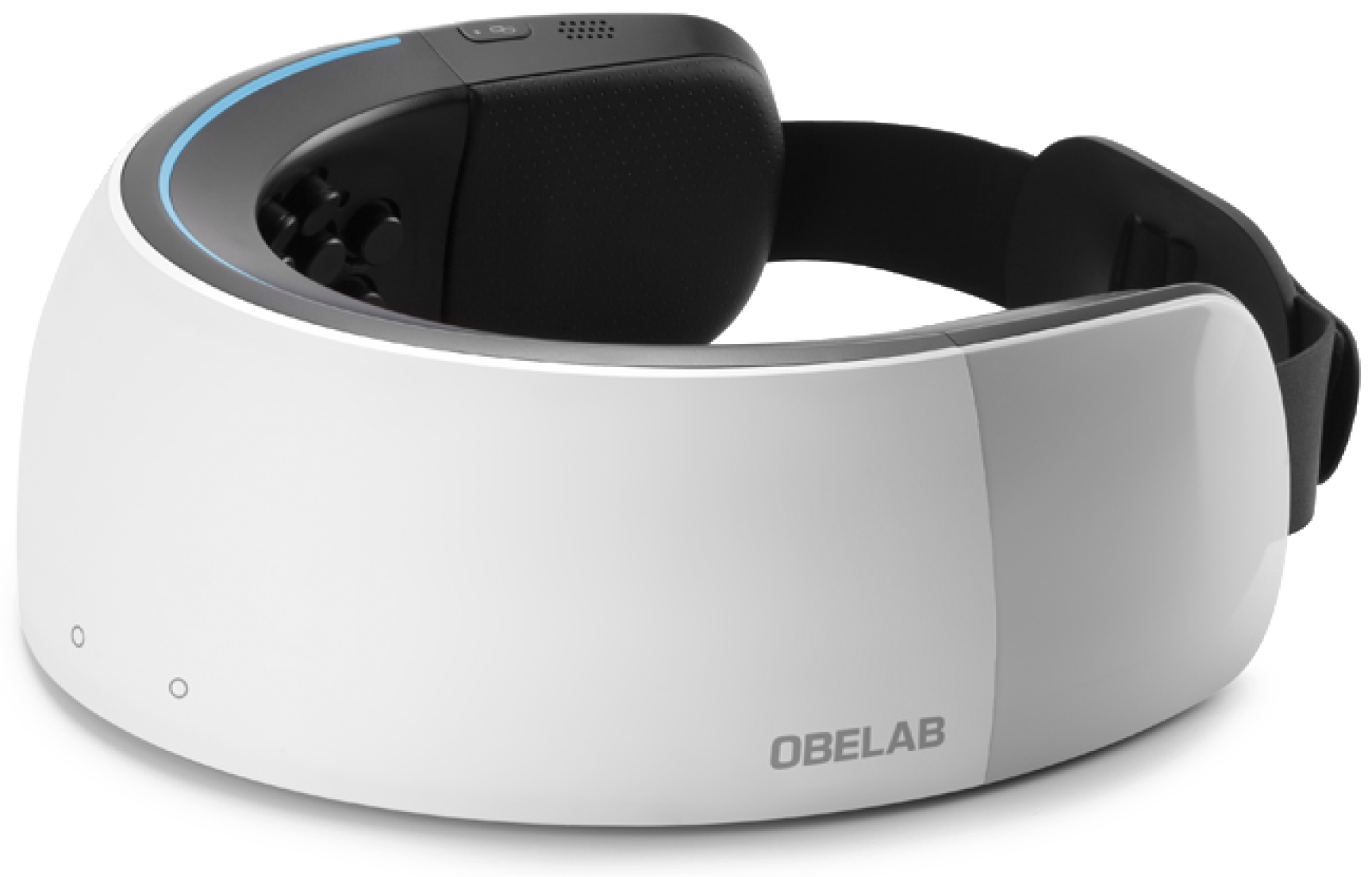
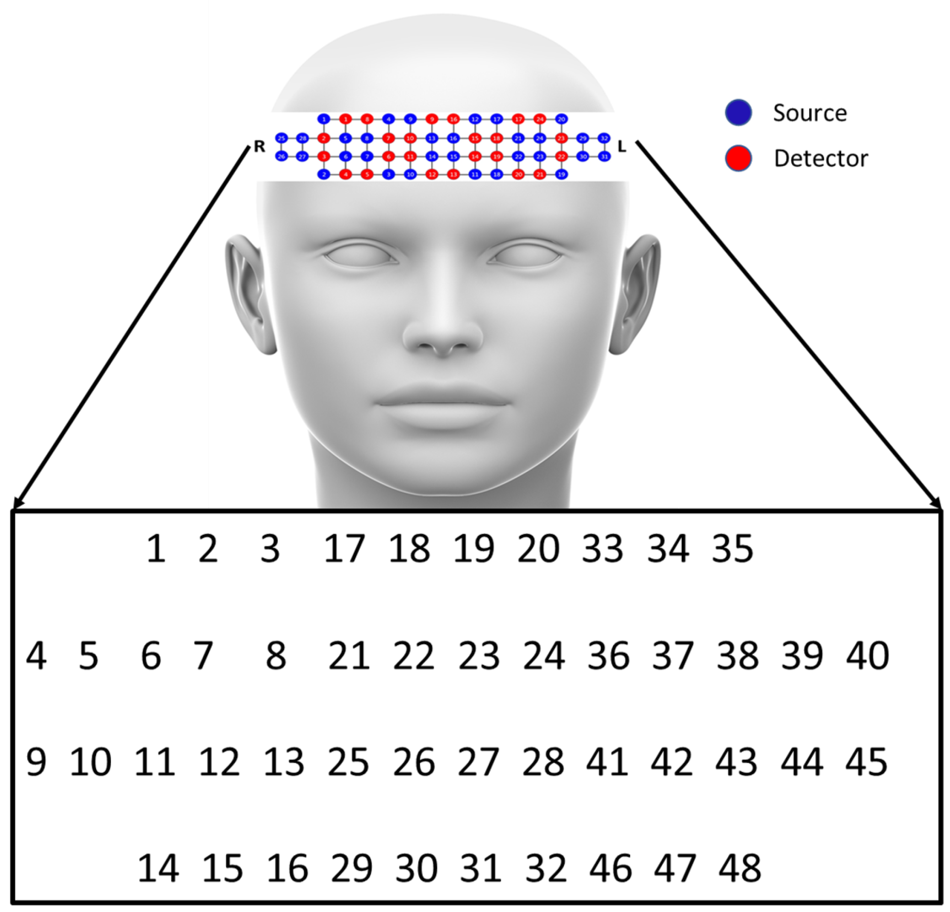
2.1. FNIRS Devices Used in the Literature

There are many devices that are used to collect fNIRS signals. Some of them are OEG-16 [35], Brite23 [36] and LIGHTNIRS [37]. In this study, we used the NIRSIT device by Obelab [38]. The device is shown in Figure 1.
NIRSIT has a total of 24 laser diode sources and 32 detectors. The relative changes in hemoglobin concentration are measured by using light attenuation of two different wavelengths: 780 and 850 nm. There are 48 primary channels in this device of which 16 are located on the right, 16 in the center and 16 on the left of the pre-frontal cortex. In addition, the device also considers the horizontal, vertical and diagonal connections between channels. Four different distances (15, 21.2, 30 and 33.5 mm) between channels are considered by the device. This results in a total of 204 channels. FNIRS data using this device are collected at the sampling rate of 8.138 Hz. The channel locations are shown in Figure 2.

2.2. Computation Methods Using Brain Activity Signals

A number of papers in the literature have employed different computational methods to analyse physiological signals related to brain activity. In this paper, we highlight some recent work which used different classification techniques to analyse these signals. Hsu et al. [39] collected electrocardiogram (ECG) signals during music listening, and classified these signals into four types of emotions (joy, tension, sadness, and peacefulness). The classification using a least squares support vector machine (LS-SVM) reached 61.52% accuracy. Lin et al. [40] used an SVM classifier to classify EEG signals into four emotional states (joy, anger, sadness, and pleasure), with up to 82.29% accuracy. Rojas et al. [41] used 69 features from fNIRS signals to classify four types of pain, reaching 94.17% accuracy using a Gaussian SVM. In another approach, instead of using one physiological signal, a combination of signals were used for classification. Daly et al. [42] used a combination of EEG, GSR and ECG signals to classify affective valence and arousal levels, reaching an average of 68.6% accuracy. Our previous work [43] also used a combination of GSR, BVP and ST signals and classified them using an artificial neural network (ANN), reaching up to 98.5% accuracy in classifying positive, neutral and negative emotions. All of these works rely on feature extraction and a feature selection process, which significantly expands the analysis time.
Some recent FNIRS studies used deep learning methods which automatically extracted features from the raw data, reducing overall computational time. Yang et al. [44] conducted a study where they collected fNIRS signals while patients with mild cognitive impairment completed three mental tasks. They applied a CNN on the signals and reached a highest accuracy of 90.62%. Ho et al. [45] also investigated effects of mental workload on fNIRS signals by applying a deep belief network (DBN) and a CNN. The classification accuracy using DBN and CNN reached 84.26% and 72.77%, respectively. Chiarelli et al. [46] used a combination of fNIRS and EEG signals for motor imagery classification. Using a deep neural network (DNN), the average classification accuracy was 83.28%. A recent study by Ma et al. [47] used a DNN to distinguish between bipolar depression and major depressive disorder from patients’ fNIRS signals. Their average classification was 96.2%. Deep learning methods have not been used extensively on fNIRS signals during emotion recognition-related tasks, especially to understand emotional reaction to different genres of music.

3. Materials and Methods

3.1. Participants and Stimuli

A total of 27 participants (17 female and 10 male) were recruited for voluntary participation in this experiment. Their mean age was 19.4, with a standard deviation of 1.5 (range: 18–24 years). All of the participants were undergraduate or postgraduate students at the Australian National University (ANU).
We used a total of 12 music pieces for this experiment which were divided into three categories: classical, instrumental and pop. These music stimuli were chosen based on some specific characteristics. After analysing a number of classical music stimuli, Hughes [48] suggested that music stimuli which have a long-lasting periodicity (phrases spanning several bars of music) have a positive influence on the brain. Therefore, in previous music therapy research, heterogenous classical music pieces have been used consisting of various different emotion colours, with the common factor being long-lasting periodicity. In this study, we chose four classical music stimuli with this feature.
Music therapy studies have predominantly seen the use of classical music stimuli with specific characteristics during therapy. However, using only one type of stimuli is not sufficient and it limits the ecological validity of the results [49]. Our aim of this work was to go beyond the specific set of music that is used to understand human response to music and extend it to other categories of music. Thus, we also chose music stimuli from instrumental and pop music genres. The instrumental music comprised instrumental and binaural beat stimuli. For our study, we chose a piece that increases gamma waves in the brain to regain focus and awareness [50], and a piece that increases alpha waves in the brain, primarily used for meditation and relaxation [51]. The other two instrumental pieces chosen were used by Hurless et al. [52] to analyse the effects of alpha and beta waves on the brain. Finally for the pop stimuli category, we chose four music pieces based on the No. 1 song of the Billboard Hot 100 year-end charts from 2014 to 2017 [53]. As the instrumental and pop music stimuli have not been used in studies before, we could not find expert annotations of these stimuli based on different musical attributes. In the absence of expert annotations, we applied our best judgement to select stimuli based on previously described criteria and a diverse range in terms of pace and emotion colour.
Table 1 shows the names of the 12 music stimuli and their corresponding genres.

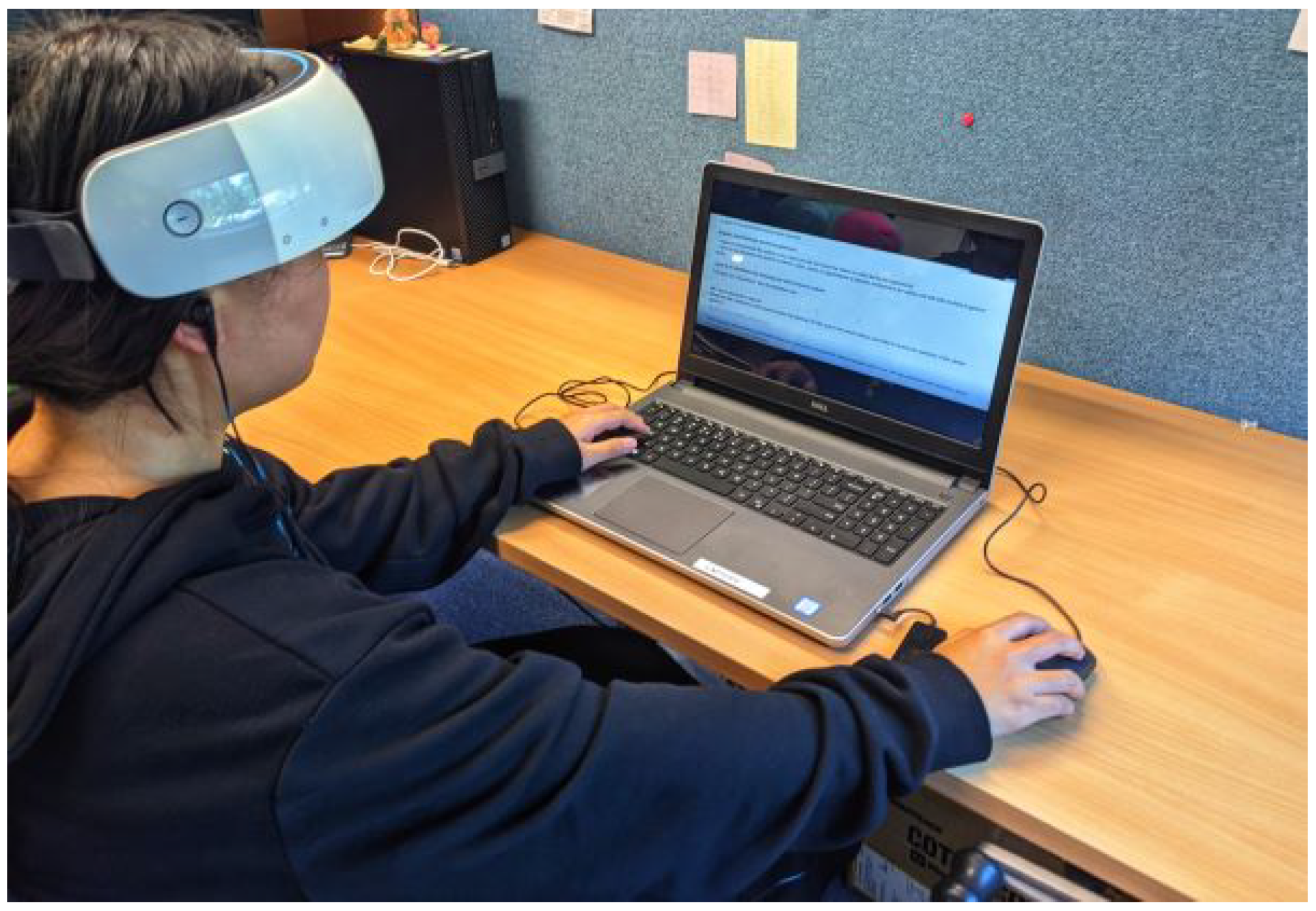
3.2. Experiment Design

This study was approved by the Human Research Ethics Committee of the Australian National University (ANU). All participants signed up for the experiment using a research participation scheme website of the ANU. After arriving at the scheduled time, participants were given an information sheet that included the description and requirements for the experiment. The document also highlighted potential risks, and how the data would be stored and used. Participants were given a consent form which they were required to sign before proceeding further in the experiment. Figure 3 shows a photo of the experimental setup.
In the first step of the experiment, participants sat in a chair in front of a 15.6 inch laptop, where they were fitted with an Obelab Nirsit device. The device was placed on the forehead of the participants. Participants were asked to move any hair from the forehead area in order to ensure good recordings. We began the calibration process by first checking in the associated tablet application to ensure all the points of the device connected properly and the application was able to visualise the blood flow in the participant’s pre-frontal cortex. We then asked them to move their head slightly in order to measure the baseline. The baseline signals were recorded for 50–53 s.
Participants answered some pre-experiment demographic questions on the laptop prior to the start of data collection. They also wore a pair of Bose QuietComfort 20 noise cancelling earphones to avoid any outside noise that might occur during the experiment. All the participants listened to all 12 pieces of music. The three genres were order balanced using the Latin square method [55] to remove any ordering bias. The music pieces within each genre were kept in the same order.
As fNIRS is a slow modality physiological signal [56], each music piece was played for two minutes in order to ensure opportunity for changes in participants’ hemodynamic response during each song. The first two minutes were chosen from the duration of each music stimuli. After participants finished listening to one music piece, they were asked to provide numeric ratings to the music pieces. These questions asked the participants to reflect on the general impression of the music and different emotions evoked by the music. The ratings were given on a 7-point Likert scale for 6 different emotion scales. The scales are (i) s a d h a p p y , (ii) d i s t u r b i n g c o m f o r t i n g , (iii) d e p r e s s i n g e x c i t i n g , (iv) u n p l e a s a n t p l e a s a n t , (v) i r r i t a t i n g s o o t h i n g , and (vi) t e n s i n g r e l a x i n g . The scales were chosen according to [57]. Continuous scales were chosen; as in the real world, human emotions are usually blended and therefore cannot be reflected using a discrete scale [58]. The entire experiment was conducted through an interactive website prepared for this purpose. The experiment took approximately one hour including device setup and participation.

3.3. Data Preprocessing

The fNIRS signals are quite sensitive to noise generated by participants’ head and body movements. They are also impacted by noise from the environment. These interference effects often result in shifts from the baseline values and fast spikes in the signals. Therefore, a number of preprocessing steps were performed on the raw signals collected from the NIRSIT device. We used the 750 nm wavelength and a 30 mm separation between channels as this is standard for many fNIRS-BCI studies [59]. From the 204 channels, the 48 primary channels were used for further analysis (based on 30 mm separation). The raw signals were first low-pass filtered at 0.1 Hz and high-pass filtered at 0.005 Hz. Then some noisy channels were rejected based on their signal-to-noise ratio (SNR). Afterwards, hemoglobin concentrations from the signals were obtained using the Modified Beer–Lambert law [60]. This method converts the near-infrared signals to HbO2, HbR and HBT (total hemoglobin) data and normalises the signals. We only used HbO2 and HbR values for each channel in further analysis. This normalisation step is necessary as it removes ’between-participant’ differences. All of these preprocessing steps were performed using the Matlab NIRSIT Analysis Tool. Finally, the signals were segmented into two-minute lengths to identify the effects of each music piece.

3.4. Feature Extraction

Classification techniques using physiological signals entail an additional step depending on the computational method being used. In deep learning methods, features are extracted automatically from the raw or pre-processed data; no additional steps are required. However, in traditional machine learning methods, a set of features needs to be extracted prior to classification. In this paper, we used two traditional machine learning methods for classification. Thus, a number of features were extracted from the pre-processed HbO2 and HBR signals. We extracted statistical features from both time and frequency domains based on a number of papers that focused on physiological signal analysis [61,62,63,64,65]. The features used in this paper are listed in Table 2.

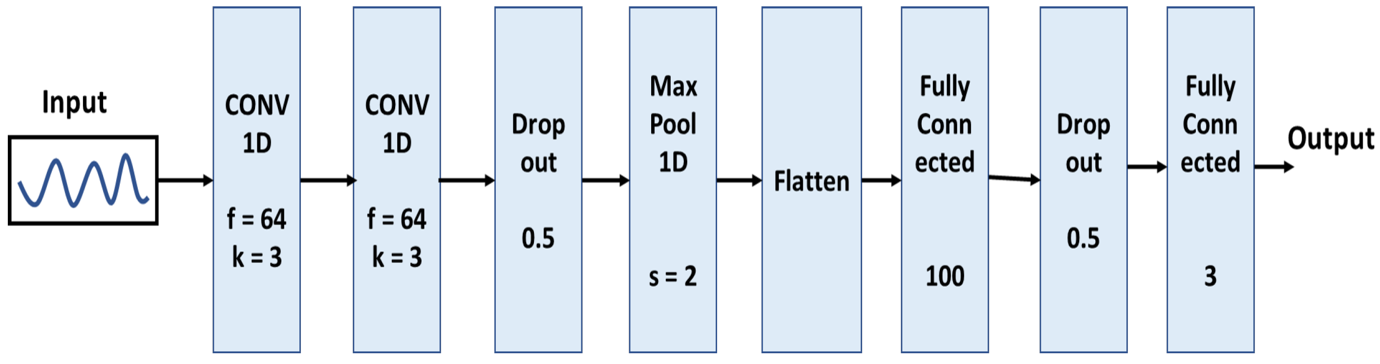
3.5. Classification Methods and Evaluation Measures

Features extracted in Section 3.4 were further analysed using two commonly used classification methods, k-nearest neighbor (KNN) and random forest (RF). We experimented with different values of parameters and picked the suitable parameters for optimum results. For the KNN method, we used k = 5 and the Chebyshev distance metric. For the RF method, we selected the number of trees to be 1000 with a maximum depth of 20. A leave-one-participant-out approach was used to evaluate the models.
Biomedical signals such as fNIRS can be represented in two formats, one-dimensional (1D) and two-dimensional (2D) data. In this paper, we used a 1D convolutional neural network (CNN) which is used for classifying time-series data. Using 1D signal data requires less memory and reduces computational complexity in comparison to 2D image data. Thus, we opted for 1D data for this analysis. We experimented with deep networks in addition to hand-crafted features because manually identifying the appropriate set of features can be highly time consuming.
The one-dimensional CNN (1D-CNN) network used the pre-processed time-series data obtained after completing the steps in Section 3.3. As this model takes in the time-series fNIRS signals as the input (without any handcrafted features), it introduces some additional challenges. Every participant’s neural structure is different, which results in high variance in their physiological signals. Even after pre-processing, there remain differences in individual responses. Therefore, the classifiers need to be trained on a per-individual basis to identify useful features from each participant.
During the pre-processing stage, it was found that each participant had different numbers of channels that recorded good-quality data. After removing some channels based on the signal-to-noise ratio, each participant was left with different numbers of channel data. Thus, the sample size of each participant was different. This produced an additional challenge to our dataset. If all the participants’ data are used together to train the model, some participants who had lower amounts of data would experience low training accuracy and this would have a significant impact on the final prediction.
In order to overcome these challenges and combine each participants’ output into the final output, we introduce an ensemble-based model. Ensemble methods are used where a new model learns the best approach to combine predictions from multiple sub-models to determine the final prediction result. This provides better generalisation and often results in better accuracy compared to using a single model. Ensemble models have been used in traditional machine learning techniques for quite some time. Recently, deep ensemble models have gained popularity as they combine the advantages of deep learning models and ensemble models. There are different techniques of creating ensemble models. Some of the techniques include bagging, boosting, and stacking. Stacked ensemble-based deep learning methods have been used in studies where time-series sequences were used [66]. They have most commonly been used in speech recognition [67,68,69] and speech emotion recognition [70]. Stacked approaches have also been used in music emotion recognition [71]. Furthermore, stacked ensemble approaches recently achieved impressive results classifying physiological signals from the DEAP dataset, which contains EEG and EMG data [72]. Therefore, in this paper, we created a stacked ensemble model using participants’ fNIRS signals.
There are multiple ways to create stacked ensemble models. Different models in the ensemble can be created using different techniques (e.g., KNN, SVM, and NN). Another way is to combine the weights of multiple neural networks with the same structure. We adopt the latter approach for our problem. In our stacked ensemble-based approach, each sub-model provides a contribution to obtain the final prediction output. The model consists of two stages. In the first stage, a model is trained on each participants’ data to create each sub-model. In the second stage, a meta-learner model is created based on the outputs from the sub-models in the first stage. The meta-learner model is then validated on a new participant’s data to make a final prediction. Thus, here we perform a subject-independent k-fold cross-validation approach to validate our model. The subject-independent cross-validation was performed by keeping one participant in the testing set for one iteration while the rest of the participants data were kept in the training set. This process was performed for every participant. This approach is also performed in similar analysis using EEG data [73].
The 1D-CNN model in the first stage was created as follows. It has two convolutional layers, one max pooling layer, one fully connected dense layer, two dropout layers and a softmax classifier. In both convolutional and dense layers, a rectified linear unit (ReLU) was used as an activation function. The dropout layers were used after the convolutional layers and the dense layer to perform better regularisation. Mean squared error was used as the loss function. For the optimisation algorithm, we used stochastic gradient descent (SGD), with a momentum of 0.9 and a decaying learning rate, with an initial learning rate of 0.01, and a mini batch size of 64. The epoch number was set to 200. The schematic diagram of the 1D CNN model is shown in Figure 4.
In the meta-learning stage, the output of the sub-models was input into a shallow neural network with one dense layer and one softmax classifier. The schematic diagram of the overall ensemble model is shown in Figure 5.
For all of the classification tasks, we report four evaluation measures. They are classification accuracy, precision, recall and f-measure. Classification accuracy reports the rate of correct classification by comparing against an independent test set. Precision is defined by the fraction of predicted labels matched, while recall measures the true positive rate. F-measure is the harmonic mean of precision and recall, and is not affected by uneven class distribution. Therefore, it is often considered a stronger measure than the arithmetic mean for reporting accuracy [74]. While classification accuracy is the most popular evaluation measure of classification models, it does not provide complete information on the predictive power and value of the model. Models with a high accuracy can sometimes have a low predictive power [75]. The classification based on participants’ subjective rating on emotions lead to an imbalance in labels, which can cause bias in the classification results. Using accuracy as the only evaluation measure is therefore not good because it does not account for the class imbalance. Thus, we report all four evaluation measures to show the complete strength of the model. Precision, recall and f-measure were computed using weighted average which accounts for any class imbalance. F-measure in particular takes the harmonic mean of precision and recall, which takes into account the class imbalance issue. This is necessary for some of the label combinations described in Section 4.
Classification was performed using the TensorFlow framework with the Python Keras library. The system specifications were an AMD Ryzen 7 3700X 8-core processor with 3.59 GHz, NVIDIA GeForce GTX 1660 SUPER GPU, 16.00 GB of RAM and a Microsoft Windows 10 Enterprise 64-bit operating system.

4. Results and Discussion

In this section, we will report the key findings derived from qualitative, quantitative, visual and computational analysis conducted on participants’ fNIRS and subjective response data.
During data pre-processing, we found that three participants’ fNIRS data were incomplete. Therefore, those participants’ data were discarded, and classification was performed using data from the remaining 24 participants. For all the subsequent computational analyses, we report two types of classification using traditional machine learning and deep learning techniques. The first is classification by music genre, where the three genres provided the three classification labels. The other is classification using the subjective rating of participants’ emotions, where we used the six different emotion ratings given by the participants as labels. We converted all of these cases into three-class classification problems. Therefore, we converted the 7-point Likert scale responses for all emotion scales into three categories (negative, neutral and positive). We applied a majority voting method to determine the final label for each music stimulus. However, for three emotion scales, only two out of the three categories received votes by the participants. The votes were either in the positive or neutral category. Thus, those three emotion scales were converted into binary classification tasks. These are d i s t u r b i n g c o m f o r t i n g (Neutral = 7, Positive = 5), d e p r e s s i n g e x c i t i n g (Neutral = 8, Positive = 4), and i r r i t a t i n g s o o t h i n g (Neutral = 8, Positive = 4). The other three remained ternary classification tasks. They are s a d h a p p y (Negative = 1, Neutral = 7, Positive = 4), u n p l e a s a n t p l e a s a n t (Negative = 1, Neutral = 6, Positive = 5), and t e n s i n g r e l a x i n g (Negative = 1, Neutral = 6, Positive = 5). It is also important to note that while the genre-based classification had the same number of samples in each class, the subjective rating-based classification had uneven numbers of samples in each class, leading to an imbalanced dataset. The other evaluation measures (precision, recall and f1-score) are useful in such cases as they account for the weight of each class.
In the following subsections, we will summarise the key messages arising from the results.

4.1. Automatic Feature Extraction Reduces Complexity and Performs Better Than Handcrafted Feature-Based Model

Table 3 shows the four evaluation measures for all seven (one genre-based and six subjective rating-based) classification problems using KNN, RF and 1D CNN model. It shows that the highest evaluation measures in all seven classification problems were achieved by the 1D CNN model. The classification accuracies of the 1D CNN model in classifying three genres using HbO2, HbR and a combination of both signals are 69.6%, 61.4% and 73.4%, respectively. The other evaluation measures also achieved highest scores using a combination of both signals (0.762 precision, 0.734 recall and 0.731 f1-score). Classification using participants’ subjective responses in a three-class category achieved up to 77.4% accuracy in classifying s a d h a p p y emotion. For the binary classification, the accuracy reached 80.5% in classifying i r r i t a t i n g s o o t h i n g emotion. Compared to the 1D CNN model, the traditional machine learning technique achieved 59.4% accuracy in ternary classification and 74.9% accuracy in binary classification. Both were achieved using all of the extracted features and the RF method. A one-way ANOVA on the accuracy results of the three methods showed high statistical significance ( p < 0.001 ).
It is important to note that in all seven cases, the highest accuracy was achieved by using both HbO2 and HbR signals together, followed by only HbO2 signals and only HbR signals. Therefore, we can conclude that using the combination of both hemoglobin concentration values is more beneficial in building a robust computational model. If it is not possible to collect both types of data, collecting only HbO2 data would be more useful than collecting HbR data. The outcome is similar to some papers in the literature where oxyhemoglobin features were shown to be more useful than deoxyhemoglobin and total hemoglobin features [76,77]. The improved performance of the 1D CNN model over KNN and RF models highlights the benefit of using deep learning techniques over traditional machine learning techniques in physiological signal analysis. In traditional machine learning methods, identifying the useful features to extract is a very difficult and time consuming step. Useful features also differ based on different physiological signals. An additional step of feature selection may also be required to identify the useful set of features. Automatic feature extraction in 1D CNN removes the requirement of these steps and thus significantly reduces the time and complexity of the process.

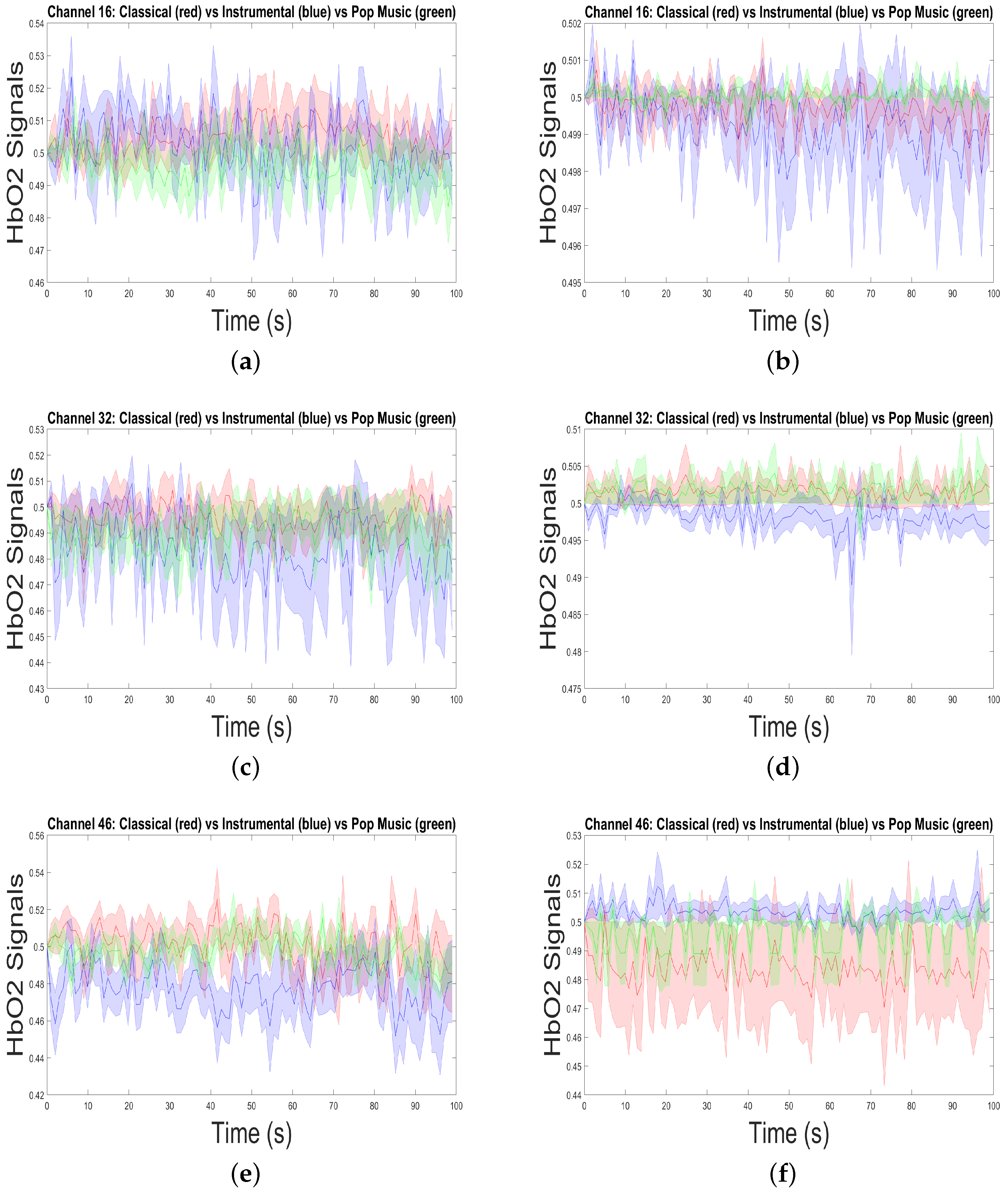
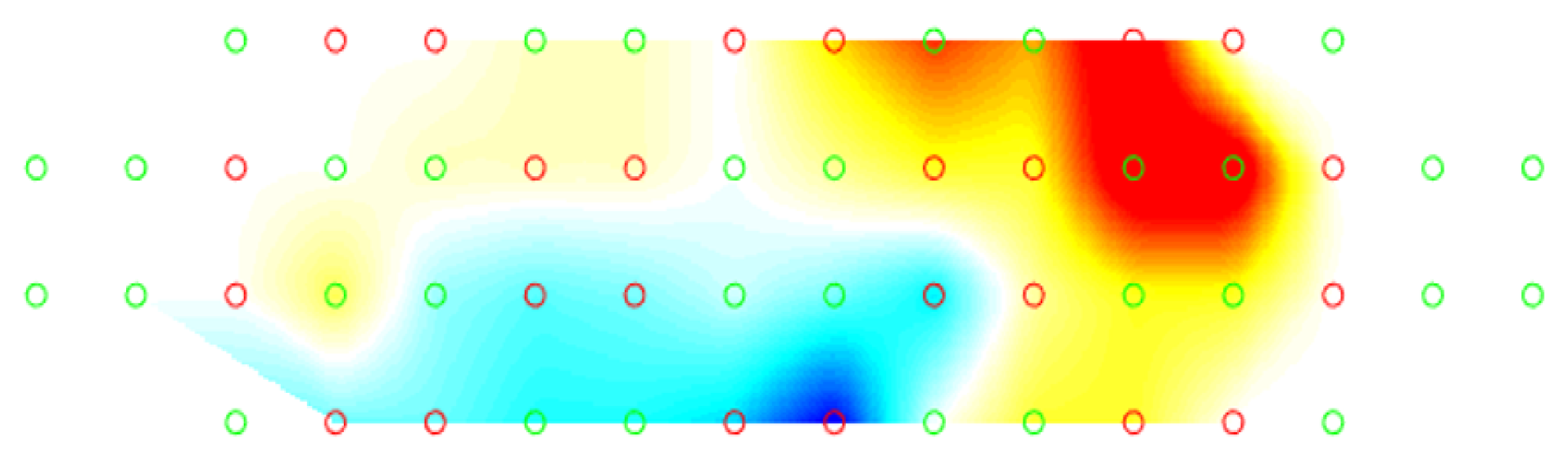
4.2. fNIRS Shows Differential Brain Responses to Music Genres

We further conducted a visual analysis of the HbO2 signals to understand how well the signals can differentiate the three music genres. We performed a timeline analysis of 100 s of signals recorded in two different stages of the experiment. The first stage signals were taken from point 900 to 1000 starting from the beginning of one genre, which is approximately 100 s after the start of the genre. The second stage was from point 2500 to 2600, which is approximately 300 s into listening to one genre. The analysis was performed on the average of all participants pre-processed HbO2 signals from three different channels. We picked channel no. 16, 32 and 46 from the left, mid and right side of the pre-frontal cortex, respectively. These channels were chosen based on their good quality of data. The signals were reshaped to set the initial value to 0.5. This value was chosen so that the increasing or decreasing trend of fNIRS response could be seen in a clear manner. The result of the timeline analysis is shown in Figure 6. The red shaded area shows participants’ fNIRS responses to classical music, while the blue and green shaded areas show responses to instrumental and pop music, respectively.
From Figure 6a,c,e, it can be seen that participants’ oxyhemoglobin response did not show much difference while they were listening to the three genres of music. These signals were captured while participants were listening to the first stimulus of each genre. However, participants’ responses were more distinguishable in Figure 6b,d,f, with a stronger response seen during classical and instrumental music listening in the mid and right pre-frontal cortex. These signals represent the responses elicited during the third stimulus of each genre. In summary, the figures show that the fNIRS signals provide a slow response in differentiating three genres. However, the responses become more prominent after the first few minutes, and show a more distinct range for the genres, especially in the mid and right pre-frontal cortex. The mid region of the pre-frontal cortex is known for decision making and maintaining emotional information within working memory [78,79]. The right pre-frontal cortex is associated with self-evaluation of the face and episodic memory [80,81].

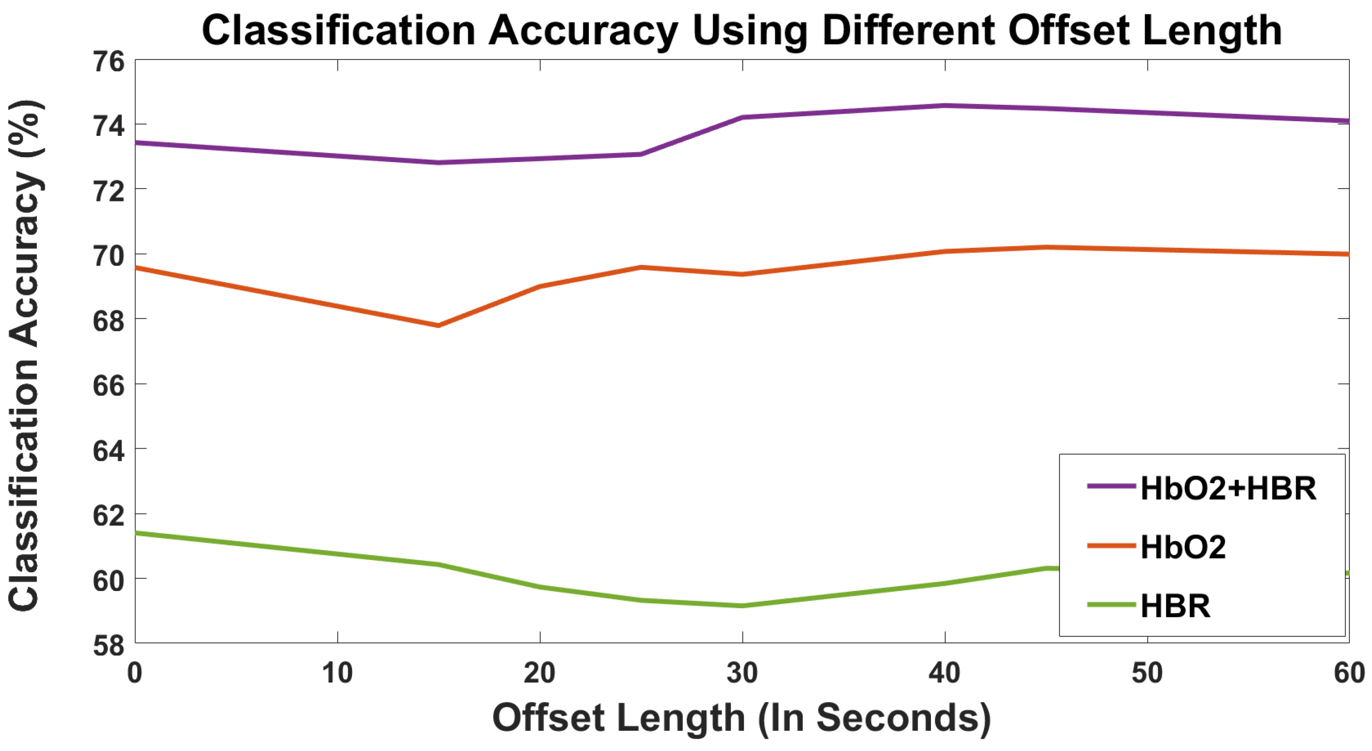
4.3. Hemodynamic Responses Are Slow Modality Signals and Show Similar Patterns While Reliving the Experience of Listening to a Music Genre

We further trained the 1D CNN model without the data from the first music track of every genre. This resulted in an increase in the classification accuracy to 75.7% using both HbO2 and HbR signals, 73.1% accuracy using only HbO2 signals, and 63.9% accuracy using only HbR signals. This could be due to the fact that fNIRS is a slow modality signal, so the effects of listening to a specific genre require time to be reflected in the signals recorded. Since the effect is seen in a delayed manner, we assumed that the effect of listening to one genre may be reflected after the playback was finished for one genre. Therefore, we further trained the model using varied offset lengths of the final stimuli in every genre. The classification result in differentiating three genres is shown in Figure 7.
We can see in Figure 7 that the classification performance decreases from the initial value of 73.4% (two minutes segment without any offset for any stimuli and not discarding first stimuli) to 72.8% using the offset length of 20 s. After that point, the accuracy starts increasing again and reaches 74.6% with the offset length of 40 s. Looking at the experiment participation of each subject, we identify this as the time period when they were completing the post-experiment questionnaire, particularly when they were answering the open-ended question of providing any comments about the music they listened to. Our assumption is that this question triggered the participants memory of listening to the music and feeling the same emotion they felt while listening to it. Thus, this effect can be seen in their hemodynamic response. The same trend can be seen using only HbO2 or HbR signals. A one-way ANOVA on the classification accuracy values showed high statistical significance ( p < 0.001 ).
Looking further at the numeric values of testing accuracy at each iteration, we noticed that the accuracy remains very similar (even if there is a slight increase, it is too close to be considered significant) or tends to drop slightly in the first 15 s in all three combinations of signals. The drop is more noticeable when a larger dataset containing both signals is used. We suspect that, if the model is trained multiple times with these different offset values using large dataset, the accuracy will mostly tend to drop in the first 15 s. In terms of the experiment design, this is the part where the participant is moving from the music listening stage to the questionnaire stage, which could be considered a break/rest point. Therefore, the effects of the music showed less prominence during this time.
This result tells us that there is a lingering effect on brain patterns while reliving the experience of listening to music from each genre. Similar findings were reported by Chen et al., where they noticed similar neural activity when participants watched and described the events of a TV show episode [82]. Our results also align with the results in Section 4.2, where we showed that the responses to different music genres became more prominent on different brain regions after the first few minutes of listening to the stimuli. This finding may be useful for future experiments that study the effects of music on the brain using fNIRS signals.

4.4. Common Assumptions about Music May Need to Be Revisited

We observed some expected and unexpected responses to some of the stimuli which was reflected in both participants’ verbal and physiological signals. For instance, the stimulus “Instrumental 1” is a binaural beat designed to enhance gamma waves on the brain, thus increasing focus and concentration on tasks. However, the majority of the votes by participants leaned towards “sad”, “unpleasant” and “tensed” rating for the three respective categories, and received neutral votes in the rest. This is contrary to our expectation as we assumed this stimulus would have a positive impact on participants’ emotion. In addition, all of the classical music mostly received neutral votes from the participants. Depending on the stimuli, we expected three out of the four stimuli to evoke a positive response, and a negative response by the other one. The stimulus “Classical 3” is a piece played in a minor key and a very sombre tone. This piece has been used in funerals. However, participants mostly voted towards neutral or positive emotions for this piece. Although this aligns with some studies that mention sad music inducing pleasant emotions [83], the findings were still surprising and interesting.
To understand this effect in a greater detail, we performed a qualitative analysis using a grounded theory approach [84] on participants’ comments provided for each music stimulus. We coded the comments into higher-level themes based on participant descriptions of the emotions they felt while listening to a particular stimulus. These codes were then divided into three categories: negative, neutral and positive. During the coding process, frequently appearing words that were considered negative were: “dislike”, “sad”, “depressing”, and “irritating”. Some of the comments highlighted as positive were: “like”, “relaxing/relaxed”, “soothing”, and “calming”. The neutral comments mostly described some features about the music, or whether they had previously heard the song or not, where the comments did not reflect participants’ emotions. Some of the common words used for neutral comments were: “familiar”, “loud”, “slow”, “fast”, and “upbeat”. The analysis was completed using NVivo 12 software. Table 4 demonstrates the number of participants providing different categories of comments on each stimulus.
Table 4 provides some interesting insights on the stimuli, which also reveals useful relationships of the music with participants’ brain activity. The classical pieces mostly received positive comments from the participants. Classical 3 stimulus also received more positive comments than negative, although it received more negative comments compared to the other stimuli. On the one hand, this stimulus received comments saying the piece is “relaxing” and “calming”, but it also received comments such as “dark” and “depressing”. This could explain the neutral ratings on the six emotion scales given by the majority of participants as the piece invoked negative emotions such as sadness and positive emotions such as relaxation at the same time. In comparison, Instrumental 1 received a majority of negative votes and comments such as “disturbing” and “irritating”. This raises a question on the effectiveness of using a gamma wave inducing binaural beats stimulus for improving focus when this causes discomfort in participants, which is likely to cause distraction and reduced focus. The pop music pieces received a mix of neutral and positive comments. However, both of these types of comments were influenced by the fact that these music tracks were more familiar (all of the participants were familiar with at least one stimulus in this category). This suggests that music stimuli invoking sad emotions or familiar music invoking positive emotion may both perform better in improving focus rather than binaural beats. Future experiments could combine music stimuli and task performance to explore this phenomenon.

4.5. Participants’ Verbal Responses on Emotional Reaction to Music Aligns with Their Hemodynamic Responses

While some of the stimuli received a different emotion label than we expected, the verbal response correlated with their hemodynamic responses. In order to analyse this, we used the image frames generated from the activation map videos by the Matlab NIRSIT Analysis Tool [85]. The activation map shows the changes of HBO2 and HbR in the prefrontal cortex over time. The map reflects the prefrontal cortext area, where the dots represents the channel locations. The colorful areas show which areas in the pre-frontal cortex were activated at a given time, and the color intensity represents the value. The frames were extracted at 25 frames/second and segmented according to the song length. Figure 8 shows a sample frame from the activation map videos.
We visualised the activation maps and found a higher HbO2 response listening to stimuli that were labelled sad compared to happy ones. Figure 9 shows sample frames of two participants listening to Instrumental 1 (received mostly negative ratings) and Pop 4 (received mostly positive ratings).
Figure 9a,c shows that for both participants, there is a higher level of HbO2 activation in the mid pre-frontal area while listening to the piece Instrumental 1. This stimulus was voted by the majority of the participants as being in either neutral or negative categories such as “tensing” and “unpleasant”. Figure 9b,c shows lower HbO2 activation listening to Pop 4, which was voted in the positive categories such as “exciting” and “soothing” by the participants. The trend is observed for other participants as well. This is similar to the work by Moghimi et al. [86], where they found larger peaks in HbO2 responses in negative emotion inducing music pieces. Our findings suggest that participants’ hemodynamic responses are correlated with their emotional reaction. Therefore, these signals can reliably be used to build computational models to provide music recommendations based on human emotional states.
The results from all parts of Section 4 indicate that participants’ hemodynamic responses are a strong indicator of their emotional responses to music. Future studies can be designed to explore these phenomena in more detail.

5. Conclusions

In this paper, we reported the results of an experiment that collected participants’ brain activity response via fNIRS signals while they listened to three different genres of music. Signals were first pre-processed using different techniques to convert the raw signals into oxyhemoglobin (HbO2) and deoxyhemoglobin (HbR) responses. Three well-known machine learning and deep learning methods (KNN, RF and 1D CNN) were applied to classify the signals. Results from our analysis show that the deep learning models achieve higher accuracy in classifying different music using their genres and participants’ subjective rating of emotions as labels. A 1D CNN model achieves 73.4% accuracy in classifying three music genres (classical, instrumental, pop) and 80.5% accuracy in classifying subjective rating of emotions ( i r r i t a t i n g s o o t h i n g ) based on the fNIRS data.
There are some limitations to our work. The number of participants may be considered small to train a deep network. The number of participants for our study has been considered reasonable in recent studies [87]. Although the initial results are promising, this needs to be analysed further. Therefore, more data will be collected in the future to build more robust models. A larger dataset will also be used to explore the complex interaction of different emotions felt by the participants during each music genre listening. As the feature engineering methods resulted in poor results, more features will be investigated along with some feature selection techniques to identify the useful set of features. The device is also sensitive to movement and noise; therefore, we had to eliminate many channels due to poor connection. Thus, further pre-processing techniques such as wavelet and Fourier transformation will be explored in order to make these models adapt to studies in the wild, where different channels may be available for different participants. Additional techniques will be explored to remove movement-related artefacts on the fly.
An additional limitation of our stacked ensemble 1D CNN method is that it assumes every participant’s model provides a useful contribution to the final model. However, there were some participants whose models resulted in poor training accuracy due to many noisy channels, a low number of samples, etc. Future work will include grid search and optimisation methods to identify the best set of models for the ensemble model. Additionally, a larger set of music stimuli will be investigated to understand if patterns similar to this study emerge across a wider range of music genres. A further future work could compare the use of musical instruments and digital instruments in the music stimuli used in this study and explore the difference in participants’ physiological response to them.
There are also certain limitations identified in the experiment design. As the instrumental and pop music stimuli have not been used in similar research before, it was not possible to come to a resolution on what common factor should be considered while choosing the stimuli in all three music genres. While classical music pieces have auditory attributes of preference established in the literature, this is not the case for instrumental and pop music pieces. Due the lack of expert annotation published on these pieces, we applied our best judgement for selection criterion. This could have introduced potential bias to our study. Future experiments will aim to gather expert annotations to identify auditory attributes such as rhythm, tempo, flow which would facilitate appropriate music stimuli choice. Another approach is to annotate based on participants physiological response to the stimuli, which may result in less nuanced labelling.
Our study provides a contribution to the field of music emotion recognition based on human hemodynamic response using automatic feature extraction with deep learning methods, which is an emerging technique. This study paves the way for a wide range of applications and future studies in musical interactions. It also identifies the usefulness of combining HbO2 and HBR signals to construct effective models. This study reveals that human brains process different genres of music differently and that we can see this in their hemodynamic response. It also reveals the strength of fNIRS signal alignment with participants’ emotional states. As fNIRS is a highly portable and non-invasive wearable technology, multiple prospects from this study can be identified which could benefit future affective computing research. Some of these are outlined below:
  • Creation of advanced wearable technology that will measure fNIRS signals and recommend music to improve participants’ emotional well-being.
  • Identification of appropriate stimuli based on participants’ physiological response for various purposes such as music therapy and task performance. As mentioned in the discussion in Section 4.4, participants’ physiological and verbal responses often do not align with pre-assumptions about the stimuli. Using their physiological responses would yield more accurate results in such cases.
  • Identification of music that has adverse effects on the brain which can be used to prevent musicogenic epilepsy.
  • Creation of wearable devices using only the regions of interest (e.g., medial pre-frontal cortex) which can be used for longer-duration experiments and continuous measurements.
Our study uncovers the effectiveness of cerebral hemodynamic responses in revealing participants affective state while listening to different music. This study has an immense potential to be used in the advancement of affective and medical computing studies, and further contribute to music therapy related studies.

Author Contributions

Conceptualization, J.S.R. and T.G.; methodology, J.S.R.; formal analysis, J.S.R.; investigation, J.S.R.; resources, J.S.R., S.C. and T.G.; data curation, J.S.R.; writing—original draft preparation, J.S.R.; writing—review and editing, J.S.R., S.C., R.J. and T.G.; supervision, T.G., R.J. and S.C.; project administration, R.J. and S.C.; funding acquisition, T.G. All authors have read and agreed to the published version of the manuscript.

Funding

This research received no external funding.

Institutional Review Board Statement

This study was approved by the Human Research Ethics Committee of the Australian National University (ANU).

Informed Consent Statement

Informed consent was obtained from all subjects involved in this study.

Data Availability Statement

Data relating to this study will be made publicly available upon completion and publication of the complete study.

Acknowledgments

The authors would like to thank all the participants who participated in this study. The authors would also like to thank Xinyu Hou, Yong Wei Lim and Zi Jin for helping with data collection.

Conflicts of Interest

The authors declare no conflict of interest.

References

  1. Juslin, P.N.; Sloboda, J.A. Music and Emotion: Theory and Research; Oxford University Press: Oxford, UK, 2001. [Google Scholar]
  2. Huang, R.H.; Shih, Y.N. Effects of background music on concentration of workers. Work 2011, 38, 383–387. [Google Scholar] [CrossRef] [PubMed]
  3. de Witte, M.; Pinho, A.d.S.; Stams, G.J.; Moonen, X.; Bos, A.E.; van Hooren, S. Music therapy for stress reduction: A systematic review and meta-analysis. Health Psychol. Rev. 2020, 16, 134–159. [Google Scholar] [CrossRef]
  4. Umbrello, M.; Sorrenti, T.; Mistraletti, G.; Formenti, P.; Chiumello, D.; Terzoni, S. Music therapy reduces stress and anxiety in critically ill patients: A systematic review of randomized clinical trials. Minerva Anestesiol. 2019, 85, 886–898. [Google Scholar] [CrossRef] [PubMed]
  5. Innes, K.E.; Selfe, T.K.; Khalsa, D.S.; Kandati, S. Meditation and music improve memory and cognitive function in adults with subjective cognitive decline: A pilot randomized controlled trial. J. Alzheimer’s Dis. 2017, 56, 899–916. [Google Scholar] [CrossRef] [PubMed]
  6. Feng, F.; Zhang, Y.; Hou, J.; Cai, J.; Jiang, Q.; Li, X.; Zhao, Q.; Li, B.A. Can music improve sleep quality in adults with primary insomnia? A systematic review and network meta-analysis. Int. J. Nurs. Stud. 2018, 77, 189–196. [Google Scholar] [CrossRef]
  7. Walden, T.A.; Harris, V.S.; Catron, T.F. How I feel: A self-report measure of emotional arousal and regulation for children. Psychol. Assess. 2003, 15, 399. [Google Scholar] [CrossRef]
  8. Cowen, A.; Keltner, D. Self-report captures 27 distinct categories of emotion bridged by continuous gradients. Proc. Natl. Acad. Sci. USA 2017, 114, E7900–E7909. [Google Scholar] [CrossRef] [Green Version]
  9. Dindar, M.; Malmberg, J.; Järvelä, S.; Haataja, E.; Kirschner, P. Matching self-reports with electrodermal activity data: Investigating temporal changes in self-regulated learning. Educ. Inf. Technol. 2020, 25, 1785–1802. [Google Scholar] [CrossRef] [Green Version]
  10. Ko, B.C. A brief review of facial emotion recognition based on visual information. Sensors 2018, 18, 401. [Google Scholar] [CrossRef]
  11. Shan, K.; Guo, J.; You, W.; Lu, D.; Bie, R. Automatic facial expression recognition based on a deep convolutional-neural-network structure. In Proceedings of the 2017 IEEE 15th International Conference on Software Engineering Research, Management and Applications (SERA), London, UK, 7–9 June 2017; pp. 123–128. [Google Scholar]
  12. Mellouk, W.; Handouzi, W. Facial emotion recognition using deep learning: Review and insights. Procedia Comput. Sci. 2020, 175, 689–694. [Google Scholar] [CrossRef]
  13. Huang, K.Y.; Wu, C.H.; Hong, Q.B.; Su, M.H.; Chen, Y.H. Speech emotion recognition using deep neural network considering verbal and nonverbal speech sounds. In Proceedings of the ICASSP 2019—2019 IEEE International Conference on Acoustics, Speech and Signal Processing (ICASSP), Brighton, UK, 12–17 May 2019; pp. 5866–5870. [Google Scholar]
  14. Dhall, A.; Sharma, G.; Goecke, R.; Gedeon, T. Emotiw 2020: Driver gaze, group emotion, student engagement and physiological signal based challenges. In Proceedings of the 2020 International Conference on Multimodal Interaction, Virtual Event, 25–29 October 2020; pp. 784–789. [Google Scholar]
  15. Noroozi, F.; Kaminska, D.; Corneanu, C.; Sapinski, T.; Escalera, S.; Anbarjafari, G. Survey on emotional body gesture recognition. IEEE Trans. Affect. Comput. 2018, 12, 505–523. [Google Scholar] [CrossRef] [Green Version]
  16. Egermann, H.; Fernando, N.; Chuen, L.; McAdams, S. Music induces universal emotion-related psychophysiological responses: Comparing Canadian listeners to Congolese Pygmies. Front. Psychol. 2015, 5, 1341. [Google Scholar] [CrossRef] [PubMed] [Green Version]
  17. Krumhansl, C.L. An exploratory study of musical emotions and psychophysiology. Can. J. Exp. Psychol. Can. Psychol. Exp. 1997, 51, 336. [Google Scholar] [CrossRef] [PubMed] [Green Version]
  18. Sudheesh, N.; Joseph, K. Investigation into the effects of music and meditation on galvanic skin response. ITBM-RBM 2000, 21, 158–163. [Google Scholar] [CrossRef]
  19. Khalfa, S.; Isabelle, P.; Jean-Pierre, B.; Manon, R. Event-related skin conductance responses to musical emotions in humans. Neurosci. Lett. 2002, 328, 145–149. [Google Scholar] [CrossRef]
  20. Hu, X.; Li, F.; Ng, T.D.J. On the Relationships between Music-induced Emotion and Physiological Signals. In Proceedings of the 19th International Society for Music Information Retrieval Conference (ISMIR 2018), Paris, France, 23–27 September 2018; pp. 362–369. [Google Scholar]
  21. Jaušovec, N.; Jaušovec, K.; Gerlič, I. The influence of Mozart’s music on brain activity in the process of learning. Clin. Neurophysiol. 2006, 117, 2703–2714. [Google Scholar] [CrossRef]
  22. Mannes, E. The Power of Music: Pioneering Discoveries in the New Science of Song; Bloomsbury Publishing: New York, NY, USA, 2011. [Google Scholar]
  23. Miendlarzewska, E.A.; Trost, W.J. How musical training affects cognitive development: Rhythm, reward and other modulating variables. Front. Neurosci. 2014, 7, 279. [Google Scholar] [CrossRef]
  24. Phneah, S.W.; Nisar, H. EEG-based alpha neurofeedback training for mood enhancement. Australas. Phys. Eng. Sci. Med. 2017, 40, 325–336. [Google Scholar] [CrossRef]
  25. Liao, C.Y.; Chen, R.C.; Liu, Q.E. Detecting Attention and Meditation EEG Utilized Deep Learning. In Proceedings of the International Conference on Intelligent Information Hiding and Multimedia Signal Processing; Springer: Berlin/Heidelberg, Germany, 2018; pp. 204–211. [Google Scholar]
  26. Coppola, G.; Toro, A.; Operto, F.F.; Ferrarioli, G.; Pisano, S.; Viggiano, A.; Verrotti, A. Mozart’s music in children with drug-refractory epileptic encephalopathies. Epilepsy Behav. 2015, 50, 18–22. [Google Scholar] [CrossRef]
  27. Forsblom, A.; Laitinen, S.; Sarkamo, T.; Tervaniemi, M. Therapeutic role of music listening in stroke rehabilitation. Ann. N. Y. Acad. Sci. 2009, 1169, 426–430. [Google Scholar] [CrossRef]
  28. Critchley, M. Musicogenic epilepsy. In Music and the Brain; Elsevier: Amsterdam, The Netherlands, 1977; pp. 344–353. [Google Scholar]
  29. Curtin, A.; Ayaz, H. Chapter 22—Neural Efficiency Metrics in Neuroergonomics: Theory and Applications. In Neuroergonomics; Ayaz, H., Dehais, F., Eds.; Academic Press: Cambridge, MA, USA, 2019; pp. 133–140. [Google Scholar] [CrossRef]
  30. Midha, S.; Maior, H.A.; Wilson, M.L.; Sharples, S. Measuring Mental Workload Variations in Office Work Tasks using fNIRS. Int. J. Hum.-Comput. Stud. 2021, 147, 102580. [Google Scholar] [CrossRef]
  31. Tang, T.B.; Chong, J.S.; Kiguchi, M.; Funane, T.; Lu, C.K. Detection of Emotional Sensitivity Using fNIRS Based Dynamic Functional Connectivity. IEEE Trans. Neural Syst. Rehabil. Eng. 2021, 29, 894–904. [Google Scholar] [CrossRef] [PubMed]
  32. Ramnani, N.; Owen, A.M. Anterior prefrontal cortex: Insights into function from anatomy and neuroimaging. Nat. Rev. Neurosci. 2004, 5, 184–194. [Google Scholar] [CrossRef]
  33. Manelis, A.; Huppert, T.J.; Rodgers, E.; Swartz, H.A.; Phillips, M.L. The role of the right prefrontal cortex in recognition of facial emotional expressions in depressed individuals: FNIRS study. J. Affect. Disord. 2019, 258, 151–158. [Google Scholar] [CrossRef]
  34. Pinti, P.; Aichelburg, C.; Gilbert, S.; Hamilton, A.; Hirsch, J.; Burgess, P.; Tachtsidis, I. A review on the use of wearable functional near-infrared spectroscopy in naturalistic environments. Jpn. Psychol. Res. 2018, 60, 347–373. [Google Scholar] [CrossRef] [PubMed] [Green Version]
  35. OEG-16 Product/Spectratech. Available online: https://www.spectratech.co.jp/En/product/productOeg16En.html (accessed on 15 February 2022).
  36. Brite23—Artinis Medical Systems|fNIRS and NIRS Devices-Blog. Available online: https://www.artinis.com/blogpost-all/category/Brite23 (accessed on 15 February 2022).
  37. LIGHTNIRS|SHIMADZU EUROPA-Shimadzu Europe. Available online: https://www.shimadzu.eu/lightnirs (accessed on 15 February 2022).
  38. OBELAB-fNIRS Devices. Available online: https://www.obelab.com/ (accessed on 15 February 2022).
  39. Hsu, Y.L.; Wang, J.S.; Chiang, W.C.; Hung, C.H. Automatic ecg-based emotion recognition in music listening. IEEE Trans. Affect. Comput. 2017, 11, 85–99. [Google Scholar] [CrossRef]
  40. Lin, Y.P.; Wang, C.H.; Jung, T.P.; Wu, T.L.; Jeng, S.K.; Duann, J.R.; Chen, J.H. EEG-based emotion recognition in music listening. IEEE Trans. Biomed. Eng. 2010, 57, 1798–1806. [Google Scholar]
  41. Rojas, R.F.; Huang, X.; Ou, K.L. A machine learning approach for the identification of a biomarker of human pain using fNIRS. Sci. Rep. 2019, 9, 5645. [Google Scholar] [CrossRef] [PubMed]
  42. Daly, I.; Williams, D.; Malik, A.; Weaver, J.; Kirke, A.; Hwang, F.; Miranda, E.; Nasuto, S.J. Personalised, multi-modal, affective state detection for hybrid brain-computer music interfacing. IEEE Trans. Affect. Comput. 2018, 11, 111–124. [Google Scholar] [CrossRef] [Green Version]
  43. Rahman, J.S.; Gedeon, T.; Caldwell, S.; Jones, R.; Jin, Z. Towards Effective Music Therapy for Mental Health Care Using Machine Learning Tools: Human Affective Reasoning and Music Genres. J. Artif. Intell. Soft Comput. Res. 2021, 11, 5–20. [Google Scholar] [CrossRef]
  44. Yang, D.; Yoo, S.H.; Kim, C.S.; Hong, K.S. Evaluation of neural degeneration biomarkers in the prefrontal cortex for early identification of patients with mild cognitive impairment: An fNIRS study. Front. Hum. Neurosci. 2019, 13, 317. [Google Scholar] [CrossRef] [PubMed] [Green Version]
  45. Ho, T.K.K.; Gwak, J.; Park, C.M.; Song, J.I. Discrimination of mental workload levels from multi-channel fNIRS using deep leaning-based approaches. IEEE Access 2019, 7, 24392–24403. [Google Scholar] [CrossRef]
  46. Chiarelli, A.M.; Croce, P.; Merla, A.; Zappasodi, F. Deep learning for hybrid EEG-fNIRS brain–computer interface: Application to motor imagery classification. J. Neural Eng. 2018, 15, 036028. [Google Scholar] [CrossRef] [PubMed]
  47. Ma, T.; Lyu, H.; Liu, J.; Xia, Y.; Qian, C.; Evans, J.; Xu, W.; Hu, J.; Hu, S.; He, S. Distinguishing Bipolar Depression from Major Depressive Disorder Using fNIRS and Deep Neural Network. Prog. Electromagn. Res. 2020, 169, 73–86. [Google Scholar] [CrossRef]
  48. Hughes, J.R.; Fino, J.J. The Mozart effect: Distinctive aspects of the music—A clue to brain coding? Clin. Electroencephalogr. 2000, 31, 94–103. [Google Scholar] [CrossRef]
  49. Harrison, L.; Loui, P. Thrills, chills, frissons, and skin orgasms: Toward an integrative model of transcendent psychophysiological experiences in music. Front. Psychol. 2014, 5, 790. [Google Scholar] [CrossRef] [Green Version]
  50. Gamma Brain Energizer—40 Hz—Clean Mental Energy—Focus Music—Binaural Beats. Available online: https://www.youtube.com/watch?v=9wrFk5vuOsk (accessed on 10 March 2018).
  51. Serotonin Release Music with Alpha Waves—Binaural Beats Relaxing Music. Available online: https://www.youtube.com/watch?v=9TPSs16DwbA (accessed on 10 March 2018).
  52. Hurless, N.; Mekic, A.; Pena, S.; Humphries, E.; Gentry, H.; Nichols, D. Music genre preference and tempo alter alpha and beta waves in human non-musicians. Impulse 2013, 24, 1–11. [Google Scholar]
  53. Billboard Year End Chart. Available online: https://www.billboard.com/charts/year-end (accessed on 10 March 2018).
  54. Lin, L.C.; Chiang, C.T.; Lee, M.W.; Mok, H.K.; Yang, Y.H.; Wu, H.C.; Tsai, C.L.; Yang, R.C. Parasympathetic activation is involved in reducing epileptiform discharges when listening to Mozart music. Clin. Neurophysiol. 2013, 124, 1528–1535. [Google Scholar] [CrossRef]
  55. Fisher, R.A. Statistical methods for research workers. In Breakthroughs in Statistics; Springer: Berlin/Heidelberg, Germany, 1992; pp. 66–70. [Google Scholar]
  56. Peck, E.M.M.; Yuksel, B.F.; Ottley, A.; Jacob, R.J.; Chang, R. Using fNIRS brain sensing to evaluate information visualization interfaces. In Proceedings of the SIGCHI Conference on Human Factors in Computing Systems, Paris, France, 27 April–2 May 2013; pp. 473–482. [Google Scholar]
  57. Walker, J.L. Subjective reactions to music and brainwave rhythms. Physiol. Psychol. 1977, 5, 483–489. [Google Scholar] [CrossRef] [Green Version]
  58. Kim, J.; André, E. Emotion recognition based on physiological changes in music listening. IEEE Trans. Pattern Anal. Mach. Intell. 2008, 30, 2067–2083. [Google Scholar] [CrossRef]
  59. Shin, J.; Kwon, J.; Choi, J.; Im, C.H. Performance enhancement of a brain-computer interface using high-density multi-distance NIRS. Sci. Rep. 2017, 7, 16545. [Google Scholar] [CrossRef] [PubMed] [Green Version]
  60. Delpy, D.T.; Cope, M.; van der Zee, P.; Arridge, S.; Wray, S.; Wyatt, J. Estimation of optical pathlength through tissue from direct time of flight measurement. Phys. Med. Biol. 1988, 33, 1433. [Google Scholar] [CrossRef] [PubMed] [Green Version]
  61. Picard, R.W.; Vyzas, E.; Healey, J. Toward machine emotional intelligence: Analysis of affective physiological state. IEEE Trans. Pattern Anal. Mach. Intell. 2001, 23, 1175–1191. [Google Scholar] [CrossRef] [Green Version]
  62. Chowdhury, R.H.; Reaz, M.B.; Ali, M.A.B.M.; Bakar, A.A.; Chellappan, K.; Chang, T.G. Surface electromyography signal processing and classification techniques. Sensors 2013, 13, 12431–12466. [Google Scholar] [CrossRef] [PubMed]
  63. Triwiyanto, T.; Wahyunggoro, O.; Nugroho, H.A.; Herianto, H. An investigation into time domain features of surface electromyography to estimate the elbow joint angle. Adv. Electr. Electron. Eng. 2017, 15, 448–458. [Google Scholar] [CrossRef]
  64. Acharya, U.R.; Hagiwara, Y.; Deshpande, S.N.; Suren, S.; Koh, J.E.W.; Oh, S.L.; Arunkumar, N.; Ciaccio, E.J.; Lim, C.M. Characterization of focal EEG signals: A review. Future Gener. Comput. Syst. 2019, 91, 290–299. [Google Scholar] [CrossRef]
  65. Rahman, J.S.; Gedeon, T.; Caldwell, S.; Jones, R. Brain Melody Informatics: Analysing Effects of Music on Brainwave Patterns. In Proceedings of the 2020 International Joint Conference on Neural Networks (IJCNN), Glasgow, UK, 19–24 July 2020; pp. 1–8. [Google Scholar]
  66. Palangi, H.; Deng, L.; Ward, R.K. Recurrent deep-stacking networks for sequence classification. In Proceedings of the 2014 IEEE China Summit & International Conference on Signal and Information Processing (ChinaSIP), Xi’an, China, 9–13 July 2014; pp. 510–514. [Google Scholar]
  67. Deng, L.; Platt, J.C. Ensemble deep learning for speech recognition. In Proceedings of the Fifteenth Annual Conference of the International Speech Communication Association, Singapore, 14–18 September 2014. [Google Scholar]
  68. Deng, L.; Tur, G.; He, X.; Hakkani-Tur, D. Use of kernel deep convex networks and end-to-end learning for spoken language understanding. In Proceedings of the 2012 IEEE Spoken Language Technology Workshop (SLT), Miami, FL, USA, 2–5 December 2012; pp. 210–215. [Google Scholar]
  69. Tur, G.; Deng, L.; Hakkani-Tür, D.; He, X. Towards deeper understanding: Deep convex networks for semantic utterance classification. In Proceedings of the 2012 IEEE International Conference on Acoustics, Speech and Signal Processing (ICASSP), Kyoto, Japan, 25–30 March 2012; pp. 5045–5048. [Google Scholar]
  70. Zvarevashe, K.; Olugbara, O.O. Recognition of Cross-Language Acoustic Emotional Valence Using Stacked Ensemble Learning. Algorithms 2020, 13, 246. [Google Scholar] [CrossRef]
  71. Malik, M.; Adavanne, S.; Drossos, K.; Virtanen, T.; Ticha, D.; Jarina, R. Stacked convolutional and recurrent neural networks for music emotion recognition. arXiv 2017, arXiv:1706.02292. [Google Scholar]
  72. Bagherzadeh, S.; Maghooli, K.; Farhadi, J.; Zangeneh Soroush, M. Emotion Recognition from Physiological Signals Using Parallel Stacked Autoencoders. Neurophysiology 2018, 50, 428–435. [Google Scholar] [CrossRef]
  73. Jiang, C.; Li, Y.; Tang, Y.; Guan, C. Enhancing EEG-based classification of depression patients using spatial information. IEEE Trans. Neural Syst. Rehabil. Eng. 2021, 29, 566–575. [Google Scholar] [CrossRef]
  74. On Average, You’re Using the Wrong Average: Geometric & Harmonic Means in Data Analysis. Available online: https://tinyurl.com/3m2dmztn/ (accessed on 10 February 2022).
  75. Valverde-Albacete, F.J.; Peláez-Moreno, C. 100% classification accuracy considered harmful: The normalized information transfer factor explains the accuracy paradox. PLoS ONE 2014, 9, e84217. [Google Scholar] [CrossRef] [PubMed] [Green Version]
  76. Bauernfeind, G.; Steyrl, D.; Brunner, C.; Müller-Putz, G.R. Single trial classification of fnirs-based brain-computer interface mental arithmetic data: A comparison between different classifiers. In Proceedings of the 2014 36th Annual International Conference of the IEEE Engineering in Medicine and Biology Society, Chicago, IL, USA, 26–30 August 2014; pp. 2004–2007. [Google Scholar]
  77. Pathan, N.S.; Foysal, M.; Alam, M.M. Efficient mental arithmetic task classification using wavelet domain statistical features and svm classifier. In Proceedings of the 2019 International Conference on Electrical, Computer and Communication Engineering (ECCE), Cox’sBazar, Bangladesh, 7–9 February 2019; pp. 1–5. [Google Scholar]
  78. Euston, D.R.; Gruber, A.J.; McNaughton, B.L. The role of medial prefrontal cortex in memory and decision making. Neuron 2012, 76, 1057–1070. [Google Scholar] [CrossRef] [PubMed] [Green Version]
  79. Smith, R.; Lane, R.D.; Alkozei, A.; Bao, J.; Smith, C.; Sanova, A.; Nettles, M.; Killgore, W.D. The role of medial prefrontal cortex in the working memory maintenance of one’s own emotional responses. Sci. Rep. 2018, 8, 3460. [Google Scholar] [CrossRef] [PubMed] [Green Version]
  80. Morita, T.; Itakura, S.; Saito, D.N.; Nakashita, S.; Harada, T.; Kochiyama, T.; Sadato, N. The role of the right prefrontal cortex in self-evaluation of the face: A functional magnetic resonance imaging study. J. Cogn. Neurosci. 2008, 20, 342–355. [Google Scholar] [CrossRef]
  81. Henson, R.; Shallice, T.; Dolan, R.J. Right prefrontal cortex and episodic memory retrieval: A functional MRI test of the monitoring hypothesis. Brain 1999, 122, 1367–1381. [Google Scholar] [CrossRef] [Green Version]
  82. Chen, J.; Leong, Y.C.; Honey, C.J.; Yong, C.H.; Norman, K.A.; Hasson, U. Shared memories reveal shared structure in neural activity across individuals. Nat. Neurosci. 2017, 20, 115–125. [Google Scholar] [CrossRef] [PubMed] [Green Version]
  83. Kawakami, A.; Furukawa, K.; Katahira, K.; Okanoya, K. Sad music induces pleasant emotion. Front. Psychol. 2013, 4, 311. [Google Scholar] [CrossRef] [Green Version]
  84. Glaser, B.G.; Strauss, A.L. Discovery of Grounded Theory: Strategies for Qualitative Research; Routledge: London, UK, 2017. [Google Scholar]
  85. OBELAB - NIRSIT Analysis Tool. Available online: http://obelab.com/upload_file/down/%5BOBELAB%5DNIRSIT_Analysis_Tool_Manual_v3.6.1_ENG.pdf (accessed on 15 February 2022).
  86. Moghimi, S.; Kushki, A.; Guerguerian, A.M.; Chau, T. Characterizing emotional response to music in the prefrontal cortex using near infrared spectroscopy. Neurosci. Lett. 2012, 525, 7–11. [Google Scholar] [CrossRef]
  87. Hossain, M.Z.; Gedeon, T.; Sankaranarayana, R. Using temporal features of observers’ physiological measures to distinguish between genuine and fake smiles. IEEE Trans. Affect. Comput. 2018, 11, 163–173. [Google Scholar] [CrossRef]
Figure 1. Obelab NIRSIT Device.
Mti 06 00035 g001
Figure 2. Nirsit Device Channel Locations at 30 mm separation.
Mti 06 00035 g002
Figure 3. Experimental Setting.
Mti 06 00035 g003
Figure 4. 1D CNN Architecture for fNIRS Signals Classification.
Mti 06 00035 g004
Figure 5. Stacked Ensemble Model Architecture for fNIRS Signals Classification.
Mti 06 00035 g005
Figure 6. Timeline Analysis of Participants HbO2 Response to Three Music Genres. (a) Channel 16: 900–1000 points. (b) Channel 16: 2500–2600 points. (c) Channel 32: 900–1000 points. (d) Channel 32: 2500–2600 points. (e) Channel 46: 900–1000 points. (f) Channel 32: 2500–2600 points.
Mti 06 00035 g006
Figure 7. Classification Accuracy Using Different Offset Lengths.
Mti 06 00035 g007
Figure 8. Frame from Activation Map Video Showing Changes in HBO2.
Mti 06 00035 g008
Figure 9. Sample Activation Map Frames: (a,b) = Frame 417 of P3 Listening to Instrumental 1 and Pop 4; (c,d) = Frame 417 of P17 Listening to Instrumental 1 and Pop 4.
Mti 06 00035 g009
Table 1. Music Stimuli Used in the Experiment.
Genre and Stimuli No.Music Stimulus Name
Classical 1Mozart Sonatas K.448 [26]
Classical 2Mozart Sonatas K.545 [54]
Classical 3F. Chopin’s “Funeral March” from Sonata in B flat minor Op. 35/2 [48]
Classical 4J.S Bach’s Suite for Orchestra No. 3 in D “Air” [48].
Instrumental 1Gamma Brain Energizer [50]
Instrumental 2Serotonin Release Music with Alpha Waves [51]
Instrumental 3“The Feeling of Jazz” by Duke Ellington [52]
Instrumental 4“YYZ” by Rush [52]
Pop 1“Happy” by Pharrell Williams
Pop 2“Uptown Funk” by Mark Ronson featuring Bruno Mars
Pop 3“Love Yourself” by Justin Bieber
Pop 4“Shape of You” by Ed Sheeran
Table 2. Features Extracted from fNIRS Signals.
Feature TypeFeature Names
Time Domain (Linear)Mean, maximum, minimum, standard deviation, interquartile range, variance, summation, skewness, kurtosis, number of peaks, root mean square, absolute summation, difference absolute standard deviation value, simple square integral, average amplitude change, means of the absolute values of the first and second differences
Time Domain (Non-Linear)Hjorth parameters (mobility), Hurst exponent
Frequency DomainMean, minimum and maximum of the first 16 points from Welch’s power spectrum
Table 3. Evaluation Measure Results Using KNN, RF and 1D CNN.
KNNRF1D CNN
LabelSignalACCPRECRECF1ACCPRECRECF1ACCPRECRECF1
c l a s s i c a l HbO20.3420.340.3420.3340.3270.3260.3270.3210.6960.7240.6960.689
i n s t r u m e n t a l HbR0.3390.3360.3390.330.3410.3420.340.3360.6140.6490.6140.602
p o p HbO2 + HbR0.3710.3780.3710.3690.3760.3740.3760.3680.7340.7620.7340.731
s a d HbO20.4950.4550.4950.4670.5530.4490.5530.4610.740.7580.740.707
n e u t r a l HbR0.490.4520.4910.4660.560.460.560.4660.670.660.670.614
h a p p y HbO2 + HbR0.5410.5120.5410.5210.5940.5380.5930.5190.7740.7860.7740.749
u n p l e a s a n t HbO20.4370.4240.4370.4270.4640.4220.4640.4280.6940.7160.6940.668
n e u t r a l HbR0.4510.4330.4510.4380.4860.4510.4860.4460.5870.5890.5870.523
p l e a s a n t HbO2 + HbR0.4890.4760.4890.4790.5170.4780.5170.4810.7340.7480.7340.717
t e n s i n g HbO20.4520.4390.4520.4420.4760.4440.4760.4460.6970.7190.6970.682
n e u t r a l HbR0.4420.4250.4420.4290.4720.4370.4720.4350.6190.6380.6190.597
r e l a x i n g HbO2 + HbR0.4790.4630.4790.4660.4910.4510.4910.4570.7190.7410.7190.708
d i s t u r b i n g HbO20.5170.5120.5160.5130.5410.5050.540.4930.7080.7340.7080.674
n e u t r a l HbR0.5180.5090.5180.5120.5490.5130.5490.4990.6260.6440.6260.546
c o m f o r t i n g HbO2 + HbR0.5390.5330.5380.5330.5440.5110.5440.4960.7180.7430.7180.684
d e p r e s s i n g HbO20.5960.5590.5950.570.6490.5550.6490.5570.7490.7470.7490.697
n e u t r a l HbR0.5950.5560.5950.5680.6510.5440.6510.550.6920.6740.6920.605
e x c i t i n g HbO2 + HbR0.6480.6330.6580.6370.6840.6680.6830.6180.770.7720.770.731
i r r i t a t i n g HbO20.7060.6380.7060.6590.7440.6310.7420.6530.7940.7910.7940.734
n e u t r a l HbR0.70.6290.70.6520.740.6270.740.6510.7690.7260.7690.69
s o o t h i n g HbO2 + HbR0.7480.7270.7470.730.7690.7490.7680.7020.8050.7990.8050.753
ACC = accuracy, PREC = precision, REC = recall, and F1 = f1-score.
Table 4. Kinds of Comments Provided by Participants on Each Music Stimuli.
StimuliNegative CommentsNeutral CommentsPositive Comments
Classical 12619
Classical 24617
Classical 39612
Classical 43519
Instrumental 11935
Instrumental 28316
Instrumental 35121
Instrumental 49810
Pop 121015
Pop 211115
Pop 33816
Pop 401215
Publisher’s Note: MDPI stays neutral with regard to jurisdictional claims in published maps and institutional affiliations.

