Optimal Design of a Ljungström Turbine for ORC Power Plants: From a 2D model to a 3D CFD Validation


Abstract
:1. Introduction
2. Materials and Methods
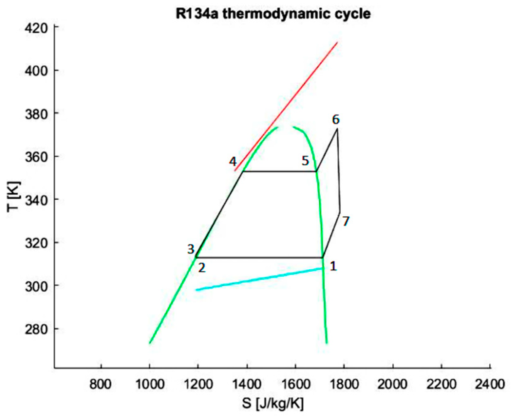
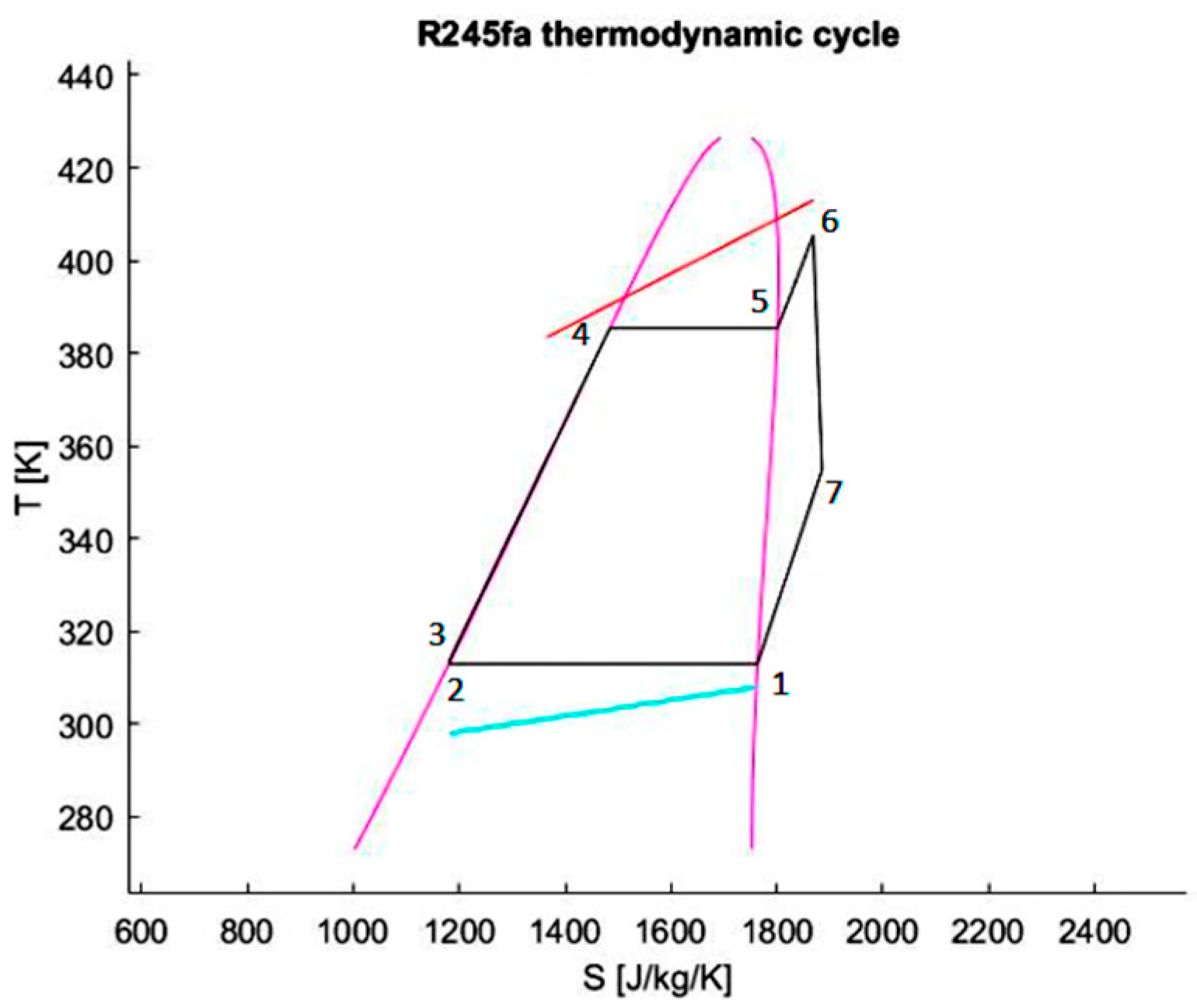
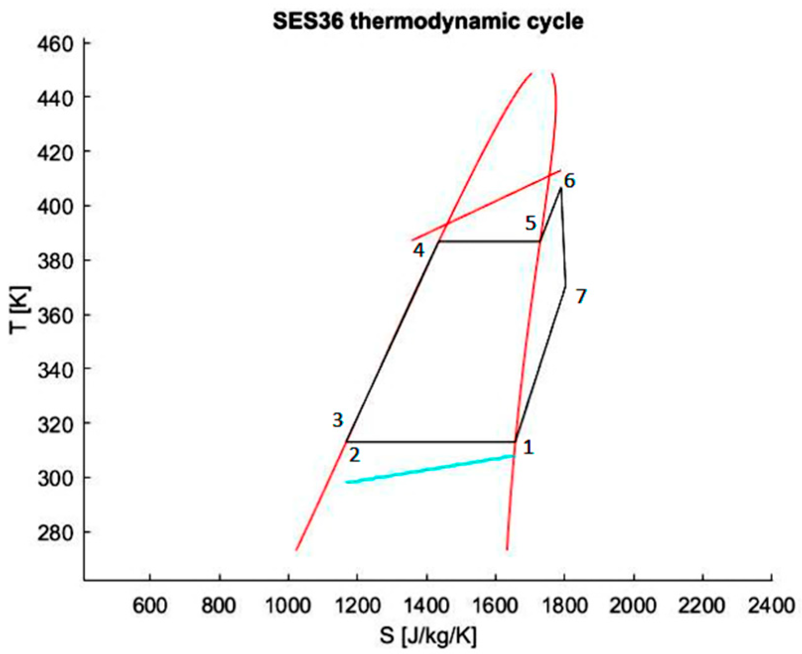
2.1. Fluid Selection
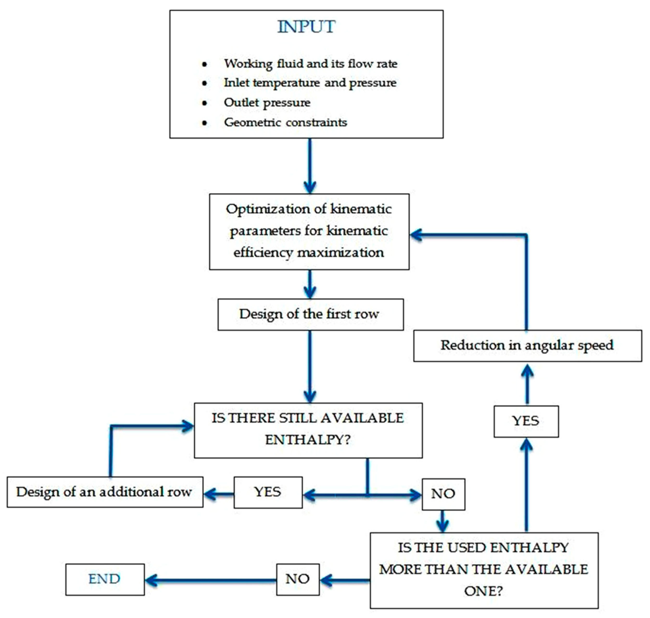
2.2. The Optimization Algorithm
- All blades, except those in the innermost ring, have the same cross-section, the same profile and the same stagger angle and, as a consequence, also have the same outlet angle:
- In all blade crowns, the ratio of the relative outlet steam velocity to the peripheral velocity at the outlet edge of the blade ring is constant and equal to:
- In all blade crowns, the ratio of the radial chord of the blade to the outlet radius is constant and equal to:
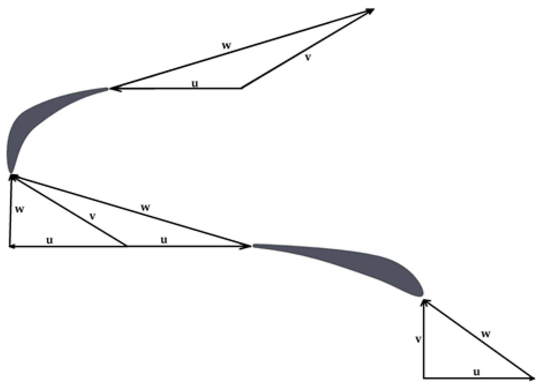
- Due to the axial symmetry of the turbine, the absolute velocity at the inlet of the first row can be considered completely radial.
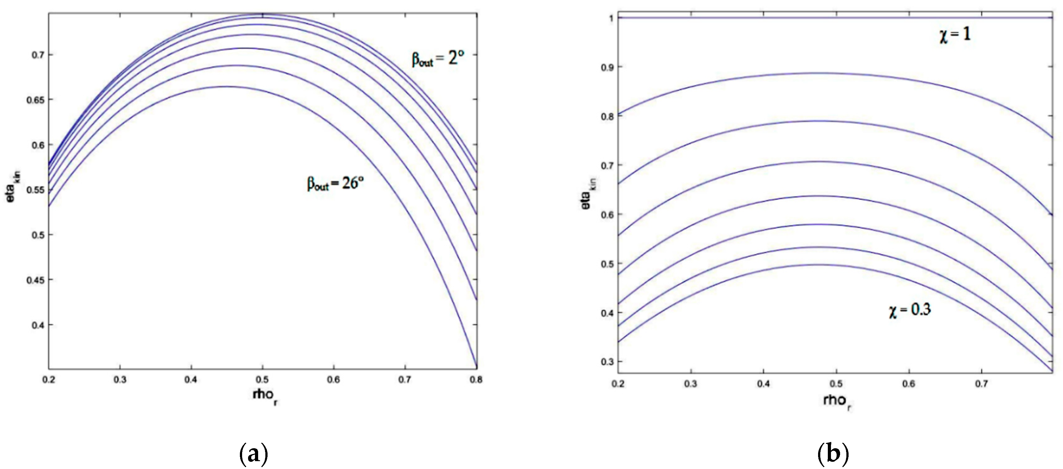
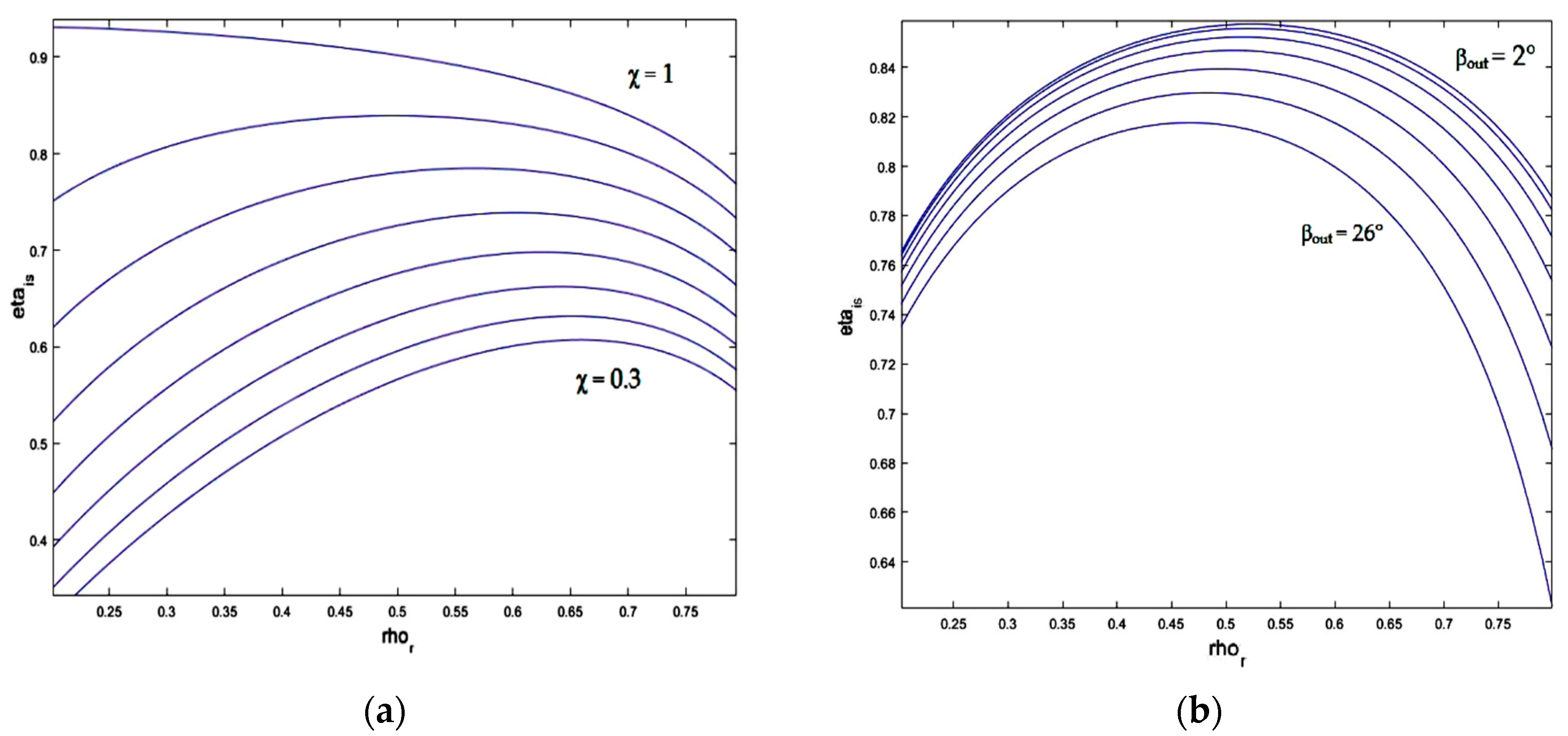
- χ = 1, meets the maximum of the efficiency for ρr = cos(βout)/2, and causes the numerator to be null. In fact, in this case uin = uout and vin = vout so that the velocity triangle is similar to that of an impulse turbine;
- βout = 0 causes the denominator to be at its maximum, in which case win = 0 because the triangle collapses onto a line.
3. Results
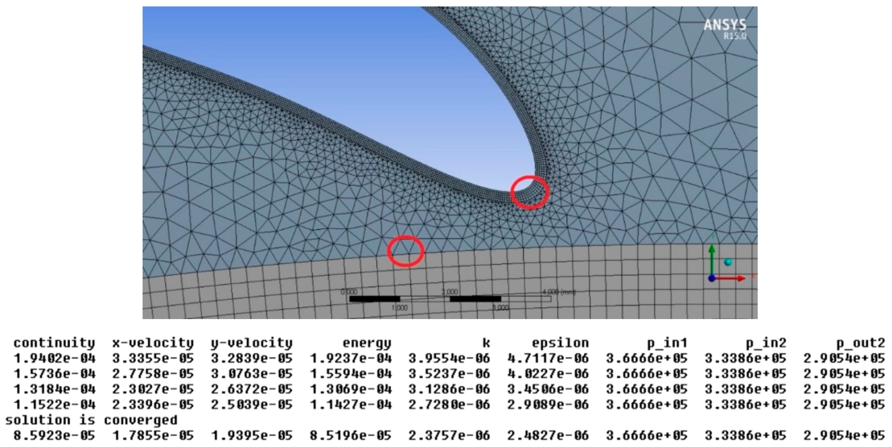
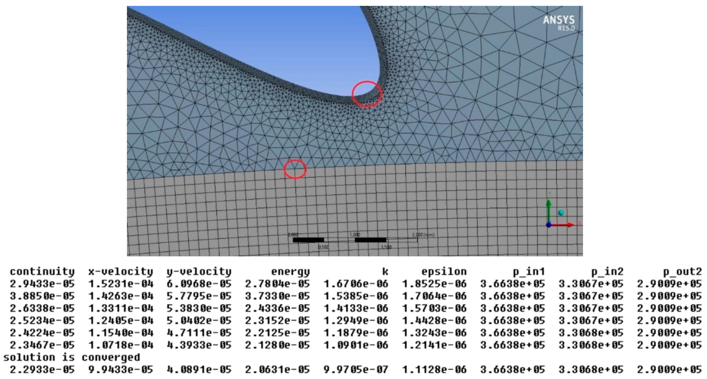
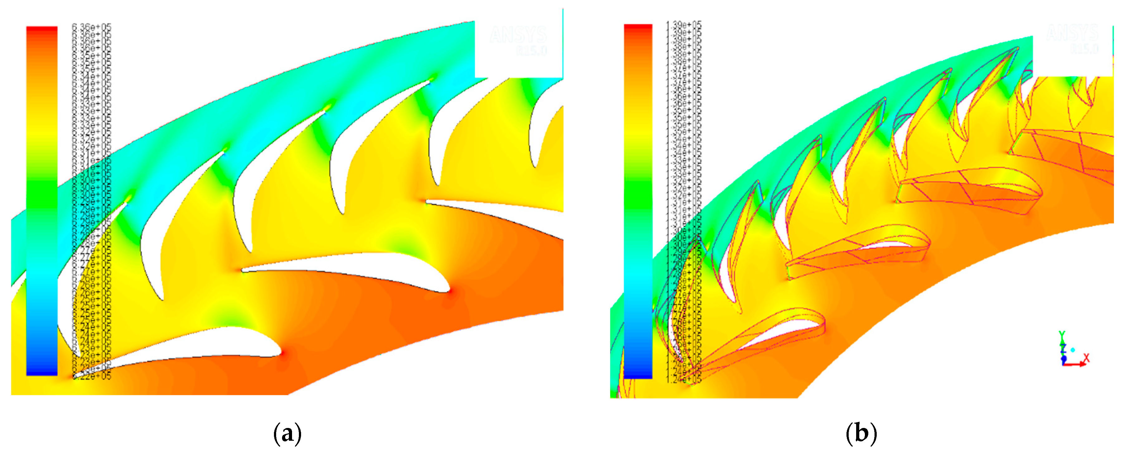
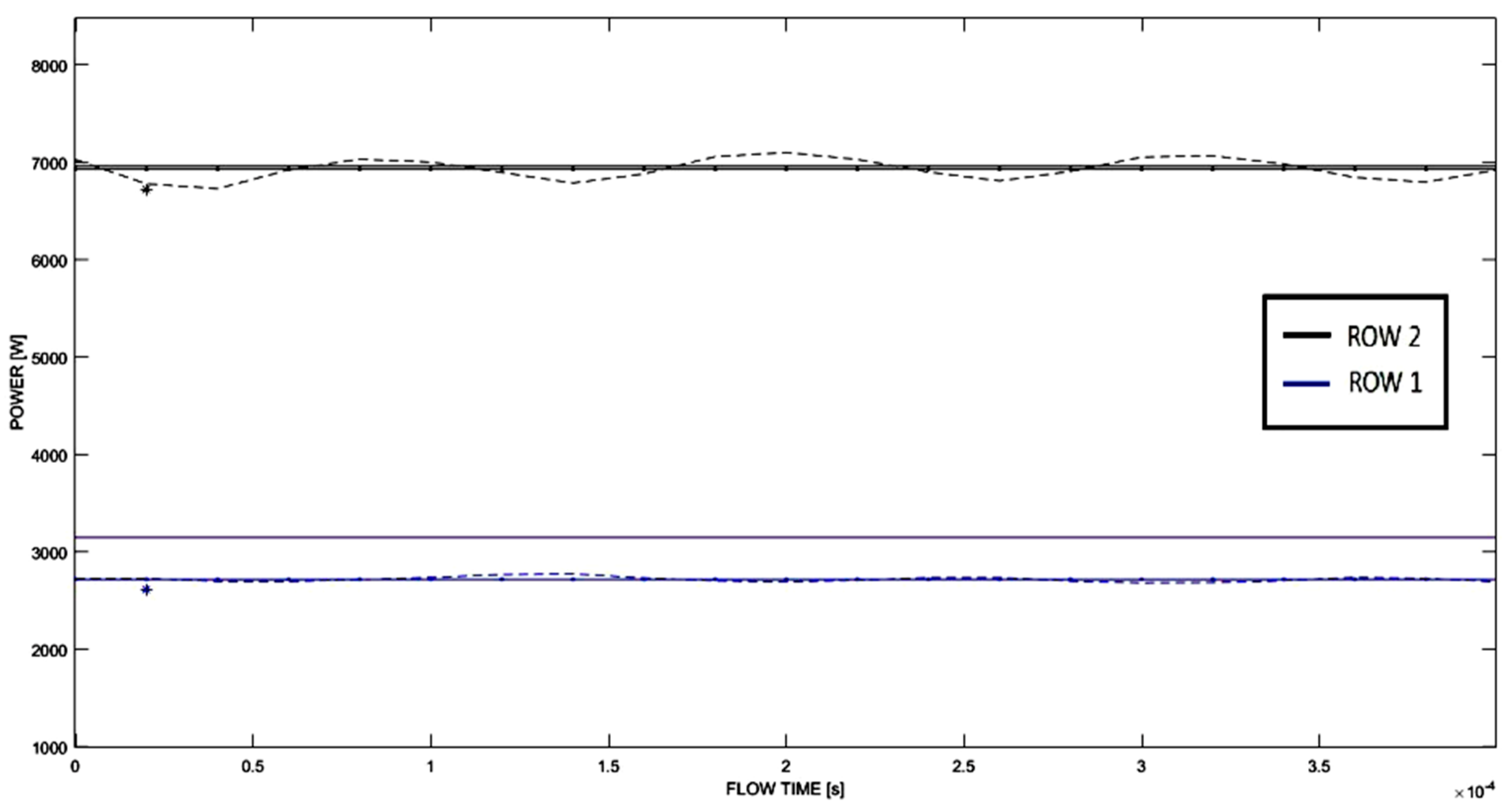
CFD Validation
4. Conclusions
Author Contributions
Funding
Conflicts of Interest
Nomenclature
| Symbol | Description | Unit of Measure | Symbol | Description | Unit of Measure |
| b | radial chord | [m] | V | absolute flow velocity | [m/s] |
| c | specific heat | [J/(kgK)] | W | relative flow velocity | [m/s] |
| ds | specific diameter | wf | working fluid | ||
| dshaft | shaft diameter | [m] | wo | working oil | |
| h | axial blade length/ enthalpy | [m] [J/kg] | β0 | relative inlet angle | |
| id | ideal | βr | expansion ratio | ||
| in | inlet | δb | blade encumbrance | ||
| l | blade chord | [m] | ε | deviation angle | |
| L | work | [J/kg] | ηcyc | cycle’s efficiency | |
| LEul | Euler’s work, [J/kg] | [J/kg] | ηis | isentropic efficiency | |
| lt | length scale, [m] | [m] | ηkin | kinematic efficiency | |
| mass flow rate | [kg/s] | ηturb | turbine efficiency | ||
| ns | specific speed | ξ | leakage factor | ||
| out | outlet | ξr | Soderberg loss coefficient | ||
| p | pressure | [Pa] | ρ | density | [kg/m3] |
| P | power | [kW] | ρr | blade to relative outlet velocity ratio | |
| r | radius | [m] | σ | blade solidity | |
| Re | Reynolds number | τall | allowable stress | [MPa] | |
| s | entropy | [J/(kgK)] | φ | flow coefficient | |
| s-s | static-to-static | χ | inlet to outlet radii ratio | ||
| T | temperature | [T] | ψ | load coefficient | |
| U | blade peripheral velocity | [m/s] | ω | angular velocity | [rpm] |
References
- Quoilin, S.; van den Broek, M.; Declaye, S.; Dewallef, P.; Lemort, V. Techno-economic survey of Organic Rankine Cycle (ORC) systems. Renew. Sustain. Energy 2013, 22, 168–186. [Google Scholar] [CrossRef] [Green Version]
- Tocci, L.; Pal, T.; Pesmazoglou, I.; Franchetti, B. Small Scale Organic Rankine Cycle (ORC): A Techno-Economic Review. Energies 2017, 10, 413. [Google Scholar] [CrossRef]
- Kang, S.H. Design and experimental study of ORC (Organic Rankine Cycle) and radial turbine using R245fa working fluid. Energy 2012, 41, 514–524. [Google Scholar] [CrossRef]
- Pei, G.; Li, Y.; Ji, J. Performance evaluation of a micro turbo-expander for application in low-temperature solar electricity generation. J. Zhejiang Univ. 2011, 12, 207–213. [Google Scholar] [CrossRef]
- Palumbo, C.F.; Barnabei, V.F.; Preziuso, E.; Coronetta, U. Design and CFD analysis of a Ljungstrom turbine for an ORC cycle in a waste heat recovery application. In Proceedings of the ECOS 2016, Portorož, Slovenia, 19–23 June 2016. [Google Scholar]
- Ljungström, F. The Development of the Ljungström Steam Turbine and Air Preheater. Proc. Inst. Mech. Eng. 1949, 160, 211–223. [Google Scholar] [CrossRef]
- Casati, E.; Vitale, S.; Pini, M.; Persico, G.; Colonna, P. Centrifugal Turbines for Mini-Organic Rankine Cycle Power Systems. J. Eng. Gas Turbine Power 2014, 136, 122607. [Google Scholar] [CrossRef]
- Pini, M.; Persico, G.; Casati, E.; Dossena, V. Preliminary design of a centrifugal turbine for ORC applications. In Proceedings of the First International Seminar on ORC Power Systems, Delft, The Netherlands, 22–23 September 2011. [Google Scholar]
- Bell, I.H.; Wronsky, J.; Quoilin, S.; Lemort, V. Pure and pseudo-pure fluid thermophysical property evaluation and the open-source thermophysical property library CoolProp. Ind. Eng. Chem. Res. 2014, 53, 2498–2508. [Google Scholar] [CrossRef] [PubMed] [Green Version]
- Franchetti, B.; Pesiridis, A.; Pesmazoglou, I.; Sciubba, E.; Tocci, L. Thermodynamic and technical criteria for the optimal selection of the working fluid in a mini-ORC. In Proceedings of the ECOS 2016, Portorož, Slovenia, 19–23 June 2016. [Google Scholar]
- Drescher, U.; Brüggemann, D. Fluid selection for the Organic Rankine Cycle (ORC) in biomass power and heat plants. Appl. Therm. Eng. 2007, 27, 223–228. [Google Scholar] [CrossRef]
- Kearton, W.J. Steam Turbine Theory and Practice: A Textbook for Engineering Students; I. Pitman & Sons: London, UK, 1958. [Google Scholar]
- Shepherd, D.G. Principles of Turbomachineryi; Macmillan Pub Co.: New York, NY, USA, 1961. [Google Scholar]
- Soderberg, C.R. Unpublished Notes; Gas Turbine Laboratory, Massachusetts Institute of Technology: Cambridge, MA, USA, 1949. [Google Scholar]
- Ainley, D.G.; Mathieson, G.C.R. An Examination of the Flow and Pressure Losses in Blade Rows of Axial-Flow Turbines; HM Stationery Office: London, UK, 1951. [Google Scholar]
- Craig, H.R.M.; Cox, H.J.A. Performance Estimation of Axial Flow Turbines. Proc. Inst. Mech. Eng. 1971, 185, 407–424. [Google Scholar] [CrossRef]
- Sciubba, E. Lezioni di Turbomacchine; Euroma La Goliardica: Rome, Italy, 2001. [Google Scholar]
- Dunham, J. A Parametric Method of Turbine Blade Profile Design. In Proceedings of the ASME International Gas Turbine Conference and Products Show, Zurich, Switzerland, 30 March–4 April 1974. [Google Scholar]
- Zweifel, O. Optimum Blade Pitch for Turbo-Machines with Special Reference to Blades of Great Curvature. Eng. Dig. 1946, 7, 358–360. [Google Scholar]
- Pini, M.; Persico, G.; Casati, E.; Dossena, V. Preliminary design of a centrifugal turbine for ORC applications. J. Eng. Gas Turbines Power 2013, 134, 042312. [Google Scholar] [CrossRef]


| Equipment | Temperature 1 [K] | Pressure 1 [Pa] | Enthalpy 1 [J/kg] | Density 1 [kg/m3] |
|---|---|---|---|---|
| Condenser (1) | 313.00 | 73,593 | 378,072 | 2.04 |
| Pump (2) | 313.00 | 73,593 | −18,013 | 725.38 |
| Economizer (3) | 313.06 | 250,885 | −17,768 | 725.52 |
| Evaporator (4) | 353.00 | 250,885 | 61,970 | 682.63 |
| Superheater (5) | 353.00 | 250,885 | 426,794 | 6.43 |
| Turbine (6) | 373.00 | 250,885 | 458,217 | 6.01 |
| Regenerator (7) | 341.04 | 73,593 | 416,033 | 1.86 |
| Equipment | Temperature 1 [K] | Pressure 1 [Pa] | Enthalpy 1 [J/kg] | Density 1 [kg/m3] |
|---|---|---|---|---|
| Condenser (1) | 313.00 | 115,093 | 363,518 | 3.35 |
| Pump (2) | 313.00 | 115,093 | 9010 | 605.85 |
| Economizer (3) | 313.09 | 366,619 | 9425 | 606.13 |
| Evaporator (4) | 353.00 | 366,619 | 108,917 | 562.19 |
| Superheater (5) | 353.00 | 366,619 | 427,177 | 10.11 |
| Turbine (6) | 373.00 | 366,619 | 468,490 | 9.35 |
| Regenerator (7) | 348.94 | 115,093 | 430,071 | 2.96 |
| Equipment | Temperature 1 [K] | Pressure 1 [Pa] | Enthalpy 1 [J/kg] | Density 1 [kg/m3] |
|---|---|---|---|---|
| Condenser (1) | 313.00 | 1012,509 | 419,363 | 49.87 |
| Pump (2) | 313.00 | 1012,509 | 256,185 | 1147.37 |
| Economizer (3) | 314.11 | 2624,797 | 257,590 | 1155.48 |
| Evaporator (4) | 353.00 | 2624,797 | 322,105 | 929.39 |
| Superheater (5) | 353.00 | 2624,797 | 428,830 | 154.37 |
| Turbine (6) | 373.00 | 2624,797 | 460,255 | 121.11 |
| Regenerator (7) | 333.93 | 1012,509 | 442,132 | 43.82 |
| Equipment | Temperature 1 [K] | Pressure 1 [Pa] | Enthalpy 1 [J/kg] | Density 1 [kg/m3] |
|---|---|---|---|---|
| Condenser (1) | 313.00 | 249,412 | 435,245 | 13.95 |
| Pump (2) | 313.00 | 249,412 | 252,838 | 1297.13 |
| Economizer (3) | 313.55 | 1648,462 | 253,916 | 1300.84 |
| Evaporator (4) | 385.44 | 1648,462 | 360,253 | 1038.29 |
| Superheater (5) | 385.44 | 1648,462 | 482,315 | 98.34 |
| Turbine (6) | 405.44 | 1648,462 | 509,011 | 84.42 |
| Regenerator (7) | 354.94 | 249,412 | 476,033 | 11.89 |
| Equipment | Temperature 1 [K] | Pressure 1 [Pa] | Enthalpy 1 [J/kg] | Density 1 [kg/m3] |
|---|---|---|---|---|
| Condenser (1) | 313.00 | 116,523 | 389,772 | 8.78 |
| Pump (2) | 313.00 | 116,523 | 233,461 | 1333.94 |
| Economizer (3) | 313.31 | 857,341 | 234,016 | 1335.99 |
| Evaporator (4) | 386.78 | 857,341 | 327,876 | 1104.87 |
| Superheater (5) | 386.78 | 857,341 | 442,402 | 63.85 |
| Turbine (6) | 406.78 | 857,341 | 466,484 | 56.91 |
| Regenerator (7) | 370.35 | 116,523 | 439,563 | 7.21 |
| Fluid | η [–] | ṁ [kg/s] | βr [–] |
|---|---|---|---|
| Cyclopentane | 9.63% | 1.35 | 3.41 |
| R601 | 9.79% | 1.50 | 3.19 |
| R134a | 11.23% | 4.03 | 2.59 |
| R245fa | 16.34% | 1.50 | 6.61 |
| SES36 | 15.46% | 1.50 | 7.36 |
| [kg/s] | Working Fluid Mass Flow Rate | τall | [MPa] | Allowable Stress at the Shaft | 80 | |
| pin | [Pa] | Inlet pressure | ωmax | [rpm] | Maximum speed | 4400 |
| pout | [Pa] | Outlet pressure | δb | [–] | Blade encumbrance | 0.85 |
| Tin | [K] | Inlet temperature | lmin | [m] | Minimum blade height | 0.01 |
| bmin | [m] | Radial chord | 0.01 | |||
| βout | [deg] | Minimum relative outlet angle | 18° |
| Fluid | n° of Rows | ns1 | ω [rpm] | Power [kW] | ηkin | ηis | χ |
|---|---|---|---|---|---|---|---|
| Cyclopentane | 6 | 0.587 | 3648 | 56 | 0.914 | 0.836 | 0.925 |
| R601 | 6 | 0.586 | 4016 | 56 | 0.897 | 0.826 | 0.909 |
| R134a | 6 | 0.434 | 3714 | 61 | 0.815 | 0.729 | 0.821 |
| R245fa | 4 | 0.499 | 9171 | 34 | 0.698 | 0.590 | 0.688 |
| SES36 | 6 | 0.350 | 4541 | 32 | 0.783 | 0.675 | 0.792 |
| Fluid | 1st Row | 2nd Row | 3rd Row | 4th Row | 5th Row | 6th Row |
|---|---|---|---|---|---|---|
| Cyclopentane | 0.010 | 0.011 | 0.011 | 0.011 | 0.011 | 0.012 |
| R601 | 0.010 | 0.010 | 0.010 | 0.009 | 0.010 | 0.010 |
| R134a | 0.011 | 0.008 | 0.006 | 0.005 | 0.004 | 0.003 |
| R245fa | 0.010 | 0.006 | 0.003 | 0.003 | ||
| SES36 | 0.010 | 0.007 | 0.005 | 0.004 | 0.004 | 0.004 |
| Parameter | Unit | 1st Row | 2nd Row | 3rd Row | 4th Row | 5th Row | 6th Row |
|---|---|---|---|---|---|---|---|
| ηis | – | 0.615 | 0.850 | 0.845 | 0.839 | 0.834 | 0.830 |
| ns | – | 0.54 | 0.31 | 0.29 | 0.27 | 0.26 | 0.26 |
| ds | – | 3.72 | 4.77 | 5.13 | 5.43 | 5.66 | 5.77 |
| uin | [m/s] | 42 | 46 | 51 | 56 | 61 | 68 |
| uout | [m/s] | 46 | 51 | 56 | 61 | 68 | 74 |
| vin | [m/s] | 29 | 54 | 60 | 66 | 72 | 79 |
| vout | [m/s] | 54 | 60 | 66 | 72 | 79 | 87 |
| win | [m/s] | 51 | 30 | 33 | 36 | 40 | 44 |
| wout | [m/s] | 96 | 106 | 116 | 128 | 141 | 155 |
| ϕin | – | 0.7 | 0.64 | 0.64 | 0.64 | 0.64 | 0.64 |
| ϕout | – | 0.64 | 0.64 | 0.64 | 0.64 | 0.64 | 0.64 |
| ψin | – | 0.00 | 0.98 | 0.98 | 0.98 | 0.98 | 0.98 |
| ψout | – | −0.98 | −0.98 | −0.98 | −0.98 | −0.98 | −0.98 |
| hin | [m] | 468,500 | 466,000 | 461,000 | 456,000 | 449,000 | 441,000 |
| hout | [m] | 466,000 | 461,000 | 456,000 | 449,000 | 441,000 | 431,000 |
| Tin | [K] | 373 | 371 | 368 | 364 | 360 | 355 |
| Tout | [K] | 371 | 368 | 364 | 360 | 355 | 349 |
| sin | [J/kgK] | 1,343 | 1,347 | 1,349 | 1,352 | 1,355 | 1,360 |
| pin | [Pa] | 366,619 | 366,040 | 292,470 | 247,050 | 201,090 | 156,400 |
| pout | [Pa] | 366,040 | 292,470 | 247,050 | 201,090 | 156,400 | 115,050 |
| ρin | [kg/m3] | 9.35 | 8.54 | 7.42 | 6.27 | 5.11 | 3.99 |
| ρout | [kg/m3] | 8.54 | 7.42 | 6.27 | 5.11 | 3.99 | 2.95 |
© 2020 by the author. Licensee MDPI, Basel, Switzerland. This article is an open access article distributed under the terms and conditions of the Creative Commons Attribution (CC BY-NC-ND) license (http://creativecommons.org/licenses/by-nc-nd/4.0/).
Share and Cite
Coronetta, U.; Sciubba, E. Optimal Design of a Ljungström Turbine for ORC Power Plants: From a 2D model to a 3D CFD Validation. Int. J. Turbomach. Propuls. Power 2020, 5, 19. https://0-doi-org.brum.beds.ac.uk/10.3390/ijtpp5030019
Coronetta U, Sciubba E. Optimal Design of a Ljungström Turbine for ORC Power Plants: From a 2D model to a 3D CFD Validation. International Journal of Turbomachinery, Propulsion and Power. 2020; 5(3):19. https://0-doi-org.brum.beds.ac.uk/10.3390/ijtpp5030019
Chicago/Turabian StyleCoronetta, Umberto, and Enrico Sciubba. 2020. "Optimal Design of a Ljungström Turbine for ORC Power Plants: From a 2D model to a 3D CFD Validation" International Journal of Turbomachinery, Propulsion and Power 5, no. 3: 19. https://0-doi-org.brum.beds.ac.uk/10.3390/ijtpp5030019