1. Introduction
Higher performance and noise requirements in modern aero-engines lead to increased by-pass ratio and slower rotating fan. Both geared and un-geared turbofans provide a solution to the challenges of higher by-pass ratios but with a very different effect on the low-pressure expansion system. The geared aero-engine enables a faster rotating low-pressure turbine (LPT) by decoupling the core and fan rotational speed. The un-geared fan will, on the other hand, have a slower rotating LPT, causing a higher stage loading or stage count to extract the same amount of work. The designer of the low-pressure expansion system, thus, has to be able to cope with a wider operational envelope in terms of swirl, stage loading, and gas temperature. The higher pressure ratio expected in the new engines also introduces thermal challenges, especially at off-design conditions.
The low-pressure expansion system includes the LPT, the turbine-rear structure (TRS), and the core exhaust nozzle. The TRS is an annular structure located downstream of the LPT, which has the mechanical function of supporting the engine-rear bearings. The TRS comprises of an outer ring, an inner ring and radial struts, so-called outlet guide vanes (OGVs). To remove the LPT exit swirl with minimal pressure losses the OGVs are aerodynamically shaped but are constrained to a minimum thickness for structural integrity and to provide passages for oil, cooling, and other service lines. As the OGVs act as the integral structural component, the thermal loads have a crucial impact on its design.
Accurate prediction and validation of the heat transfer in the TRS are hence crucial for future engine designs. Here, the newly established Chalmers University TRS-dedicated experimental facility provides conditions that enable accurate heat transfer measurement which is otherwise difficult in full-scale testing. The facility operates continuously at room temperature and can produce engine representative conditions in terms of the LPT channel Reynolds numbers and the upstream annular LPT turbulence and outlet swirl angles. Reynolds number is based on channel height and axial velocity. The commissioning of the facility is described in detail by Rojo et al. [
1,
2].
The heat transfer measurement approach used in the present study is based on techniques previously utilized at Chalmers. Initially, in an intermediate turbine duct by Arroyo et al. [
3] and by Rojo et al. [
4]. The method was later expanded for work in a linear cascade by Rojo et al. [
5] and Wang et al. [
6]. Primarily, infrared thermography (IRT) was used in mentioned studies with a variation in approach to achieve an artificial heat flux. IRT is one of the most accurate non-intrusive temperature measurement techniques but requires careful consideration to mitigate some specific uncertainties associated with it.
When measuring the object’s surface temperature with IRT, one potentially large bias error is the background radiation. However, the background radiation can be arduous to define due to it dependency of surrounding properties such as temperature, emissivity, and shape. Due to this complexity it is often simplified with a single emissivity or ignored. One method to estimate the background radiations can be achieved by raising the facility operational temperature while keeping heat flux constant over the test geometry. Another method to overcome the background radiation measurement challenges is to use a reflective marker array (RMA) utilised by Kirollos and Povey [
7]. This technique employs low emissivity circular markers on a highly emissive surface to calculated the background radiation.
An effective calibration method design remains an essential procedure in IR camera measurements to enable the user to obtain the most substantial information from an acquired image. A comparison of advanced calibration methods for an IR camera such as the 2-point, multi-point, and telops have been discussed in detail by Marcotte et al. [
8], with their implications on non-uniformity correction (NUC) and radiometry.
Nevertheless, to achieve maximum temperature accuracy and to accommodate for camera array drift, optical settings changes, etc., there is often a need for an in-situ calibration. This is usually performed by installing one or more thermocouples in the actual test specimen. However, mounting a sensor on the test specimen can have inherent uncertainties from wall gradients due to the intrusive nature of the temperature sensor and positioning. To overcome this challenge, Elfner et al. [
9] proposed an in-situ calibration with an externally mounted reference in the view of the IR camera but not mounted on a heated body.
2. Approach
To study the heat transfer on an OGV in the OGV-LPT test facility, a general design evaluation of the instrumentation was carried out. This was firstly performed by formulating a one-dimensional expression of the set-up where effects on total uncertainty from individual measurement and manufacturing limitation could be quickly evaluated using Taylor series error propagation. In an iterative process, the experimental set-up was configured for minimal measurement uncertainty of the convective surface heat transfer coefficient . The conditions during testing are representative of a mid-sized commercial jet engine with a channel height Reynolds Number of 235000 and three different throttle settings which are represented by variations in flow coefficients of the upstream LPT. During the post-processing of the data, three-dimensional effects such as in-wall heat flux were incorporated by a finite element simulation (FEM) as well as and background radiation by a version of the RMA method.
3. Experimental Test Facility
Chalmers LPT-OGV test facility is a semi-closed annular TRS test facility, the schematic for which is shown in
Figure 1. The flow is driven by a 250-kW centrifugal fan. Most of the input energy is taken up by the LPT which is regulated by a hydraulic brake. The facility is capable of continuous operation at room temperature and pressure at Reynolds numbers up to 465000. The TRS shown in
Figure 2, consists of 12 OGVs mounted with 30-degree spacing. The TRS is instrumented with two traversing systems providing near full-volume access. The baseline instrumentation is multi-hole pressure probes and surface pressure taps on the OGV. The aero surfaces in the OGV, LPT, and stators are designed by GKN Aerospace while the facility and instrumentation were designed at Chalmers. It should be noted that the aero surfaces do not relate to any GKN Aerospace product characteristics but were designed solely for the experimental facility. Further details on the design and validation of the facility are provided by Rojo et al. [
1,
2], and by Jonsson et al. [
10].
4. Heat Transfer Implementation
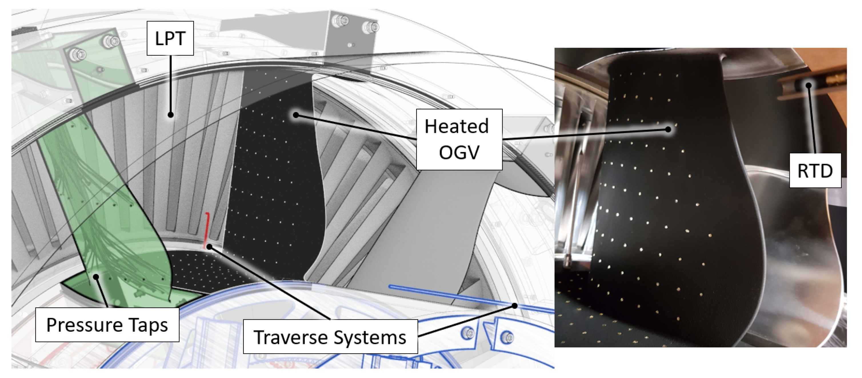
For this study, one OGV was instrumented for heat transfer measurements and is shown in
Figure 2. This OGV was manufactured with internal water channels using stereolithography (SLA). The channels are made to provide internal warm water circulation for heating the vane and providing a heat flux to the ambient colder airflow. Schematics of the instrumented OGV are shown in
Figure 3. The aero-side surface of the vane was coated with a thin layer of a high-emissivity and low-reflectivity coating (Nextel 6081) to enable highly accurate surface temperature measurement by a Phoenix 320 MWIR camera. Gold leaf markers with high reflectivity shown as dots in
Figure 2 were used for geometrical reference and evaluation of the effective background temperature, in a very similar manner to Kirollos et al. [
7]. Reference temperatures in free-stream air and channel water were measured with calibrated resistance temperature detectors (RTDs) with a traceable uncertainty of ±0.015 K following IEC 60751 [
11]. The heat transfer distribution is later obtained by solving the three-dimensional conjugate heat transfer from the vane to the airflow.
4.1. One-Dimensional Formulation of OGV Wall Heat Transfer
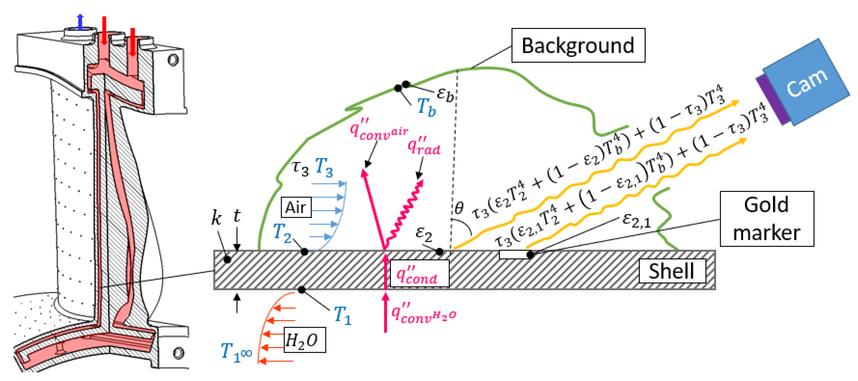
Figure 3 shows the one-dimensional simplification of the OGV wall and measurement implementation with the heat flux going from the warm water channel to the cold air stream through the shell. The warm waterside has the subindex 1, the surface of the OGV has the subindex 2 and the air has the subindex 3. The background temperature and emissivity are indexed with b. The desired quantity is the convective heat transfer on the surface
. This is calculated by subtracting the conductive heat flux
with the radiative heat flux
. The
is measured by the wall temperature difference over the shell. The radiative heat flux is described by
and is arguably the most challenging quantity to measure, as further discussed in this work. The effects of the transmissivity air
are compensated for via the in-situ calibration later described in
Section 4.5.
Heat fluxes
,
and
for this case are defined in Equation (
1) where
is the Stefan—Boltzmann constant,
is the surface emissivity,
is the equivalent background temperature,
t the shell thickness and
k thermal conductivity. Performing an energy balance and solving for
provides Equation (
2) for the convective heat transfer coefficient on the air side.
To quantify error propagation from each independent variable in Equation (
2) the Taylor series method as seen in ASME PTC19.1 [
12] has been used and is defined in Equation (
3).
Equation (
2) represents an idealised one-dimensional approximation and has been used for the design of the experiment. Together with Equation (
3) the total uncertainty and key independent contributors could be identified. Equation (
3) was evaluated using MATLAB
® software package and the symbolic expression toolbox. The following sections provide a description of the implementation and consideration for each independent variable required in Equation (
2).
4.2. Water-Side Temperature
The inner wall temperature
in Equation (
2) is not directly measured. Instead, the inlet water temperature is measured by an RTD at the inlet and the wall temperature is assumed to be constant over the instrumented vane. This is a valid assumption if two conditions are met. Firstly, the inner wall water-side thermal heat transfer coefficient is infinitely large. Secondly, there are no water temperature changes along with the flow in the water channel. The effect of the first assumption is evaluated by comparing the estimated heat flux
shown in Equation (
4) to the case of infinitely high inner wall heat transfer coefficient
, as shown in Equation (
5). The comparison between the two is formulated in Equation (
6) and provides an assessment of the bias error
caused by the first assumption. Note that the radiative heat flux is neglected in
as performed by Arroyo et al. [
3], this provides a more conservative assessment of the bias error.
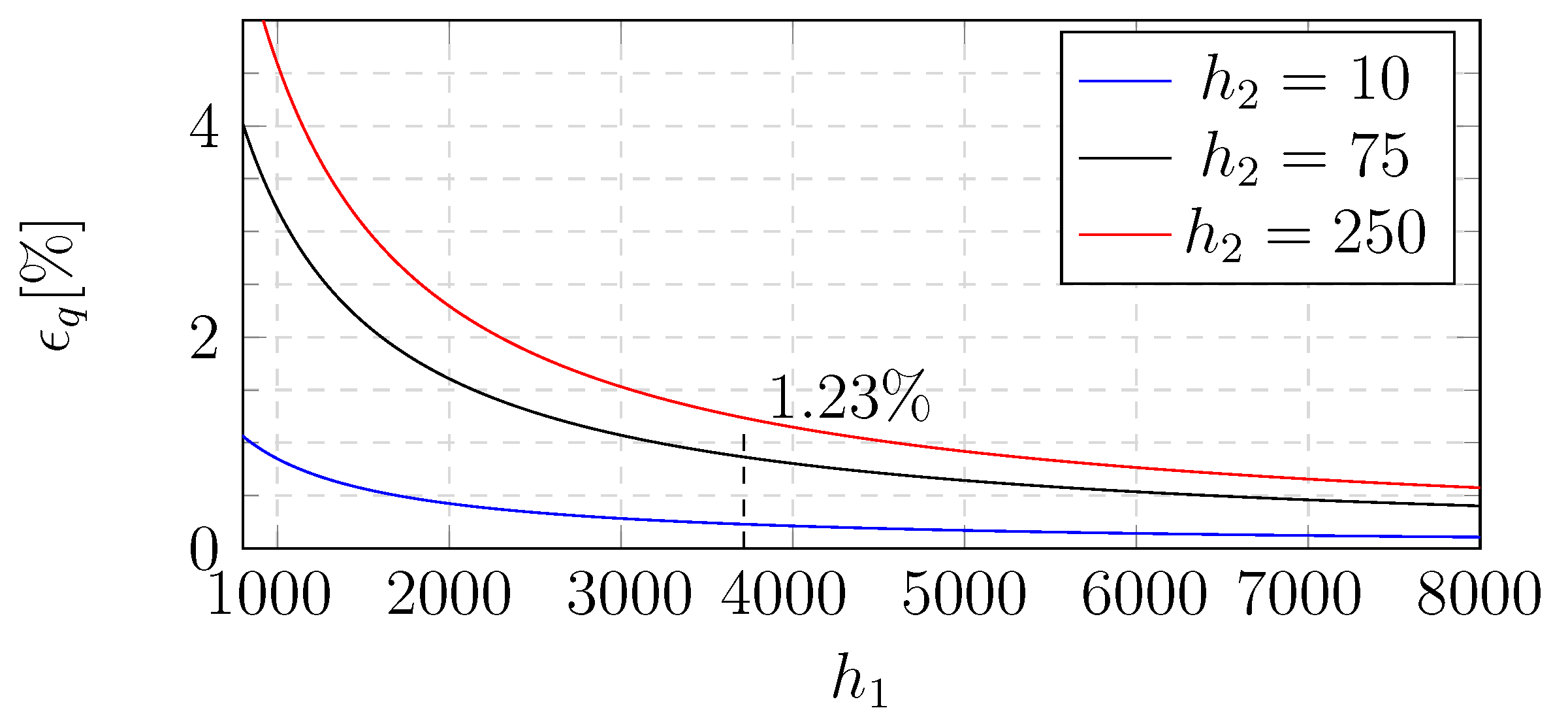
The inner wall heat transfer
can be estimated by fully developed turbulent channel flow as channel height Reynolds numbers are approximately
and a settling length of 10–30 channel heights. To maximise the inner wall heat transfer coefficient
, the inner wall water velocity was increased so the pressure drop was near the OGV shell burst pressure. At the observed peak surface heat transfer
of 250 W/(m
K) and inner wall heat transfer
W/(m
K), the uncertainty
is less than 1.3%.
Figure 4 shows the range of bias errors with different air and water heat transfer coefficient. The black dashed vertical line shows the internal heat transfer coefficient in the OGV. It can be observed that the bias error scales with the air-side heat transfer coefficient. The change of water channel mean temperature along the OGV was calculated using energy conservation and was found to be negligible.
4.3. Shell Thickness t
Using modern SLA printers, the minimal wall thickness that could be manufactured within acceptable uncertainty of was 4 mm. The shell thickness variation was measured after applying the surface coating. An Olympus 38DL Plus ultrasound thickness gauge was used at 200 locations. A systematic thickness increase of 1.5% was found at locations with the highest curvature at the leading edge. Thickness variation due to thermal expansion is estimated to be well under 0.1%.
4.4. Shell Thermal Conductivity k
The thermal conductivity of the vane material was measured by HotDisk AB following ISO22007-2 [
13] with an uncertainty of 2–5%. The measurements were performed for several material samples with different build directions. To minimise the effect of the conductivity variation due to water absorption by the epoxy resin, the vane was only subjected to the water during experiments. However, possible moisture and ageing effects still remain uncertain. The high-emissivity coating is polymer based and is estimated to have a conductivity within ±30% of the shell material. As the paint contributes to less than 3% of wall thickness the additional wall thermal conductivity uncertainty from the paint is estimated to be less than 0.1%.
4.5. Surface Temperature
The IR camera provides sensor voltage counts in a matrix format
which was converted to temperature
T by applying a fourth-order non-uniformity correction (NUC) and fifth-order calibration polynomial
P. These are defined in Equation (
7),
is the unobserved error or also known as residuals from the regression.
To calculate the
function and the polynomial
P, two calibrators were built, with the schematics of both shown in
Figure 5. The first calibrator consists of a well-isolated enclosure with optical access to a 30-mm thick flat aluminium plate coated with Nextel coating. The second is a well isolated Nextel coated 50 mm diameter copper cylinder with a door to keep the cylinder at a uniform temperature when not in use. The first device was used to construct the calibration. The second device was used for intermediate controls of the camera calibration while working with the camera. The temperature of both calibrator metal cores is measured by RTDs. In the aluminium plate three RTDs, two in the centre and one near the outer edge, were used while in the copper only one in the centre was used. The temperature management system (TMS) controls the core temperature and triggers the camera when stable temperature conditions are reached. When triggered, the camera captures 1000 frames and the calibration is obtained for every camera lens and focal settings. The properties of the surface coating are captured in the in-house calibration as both calibrator and test geometry are coated with the same coating.
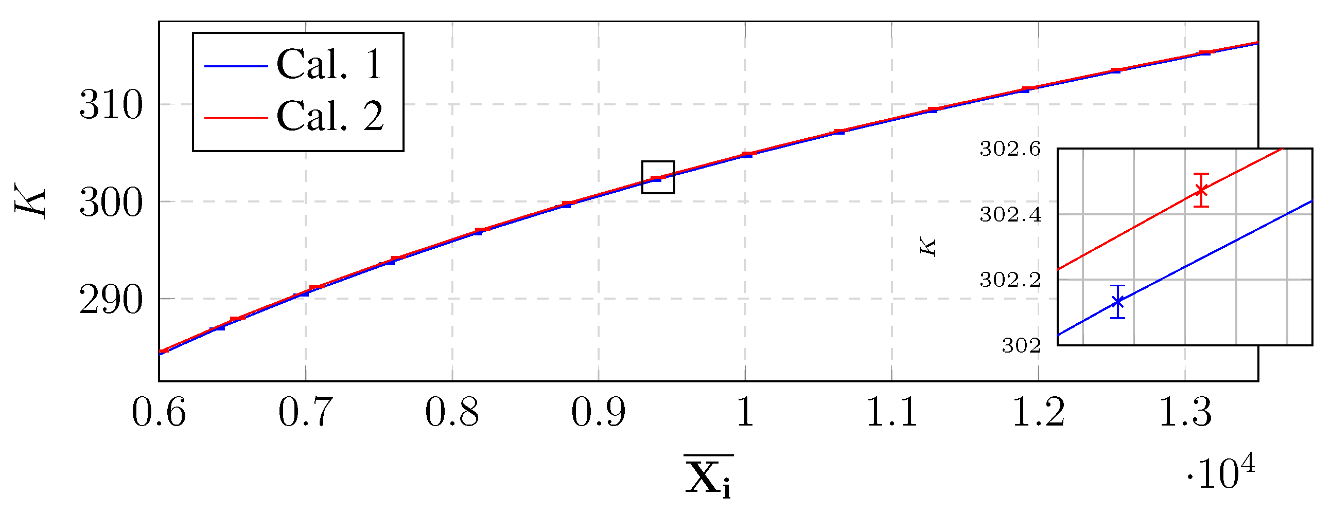
The effects of ambient temperature, focal changes, or camera background on the in-house calibration were evaluated by cross-checking camera performance several calibrations and the two calibrators. Changes such as different camera orientation, optical focus, and temperatures expected during the experiment were tested. Temperature changes to optics could lead to a near-uniform average offset of 1 K while changing focus could lead to a non-uniform offset of 0.3 K. This offset arises from the change of radiation from internals of the optics as well as narcissus effects [
14] when the focus was changed. Variation due to camera orientation or background radiation was not detectable. Two repeated calibrations with different optical focus settings are shown in
Figure 6, where the error bars show the maximum deviation from mean within the measurement point.
The bias error caused by optics temperature variation was compensated by an in-situ calibration but the effect from lens focus had to be incorporated in the NUC. In-situ reference is an RTD painted with Nextel 6081 located in the free-stream and can be seen in the upper left corner in
Figure 2. The sensor is shielded from radiation from the OGV with a reflective cover and was traversed to the camera field of view during sampling.
4.6. Emissivity Directionality and Temperature Dependence
The emissivity
of a surface is dependent on view direction
, surface temperature
T and wavelength
. Tang-Kwor et al. [
15] showed that Nextel 6081 coating has a low temperature dependency and proposed an average value of
. The calibration method used in this work excludes the effect wavelength dependency as the same camera and surface are used for both calibration and measurement. The angular dependency
is not covered in the camera calibration and was experimentally evaluated using Equation (
8).
is the camera-perceived temperature with increased
,
is the perceived temperature at
and
is the background temperature.
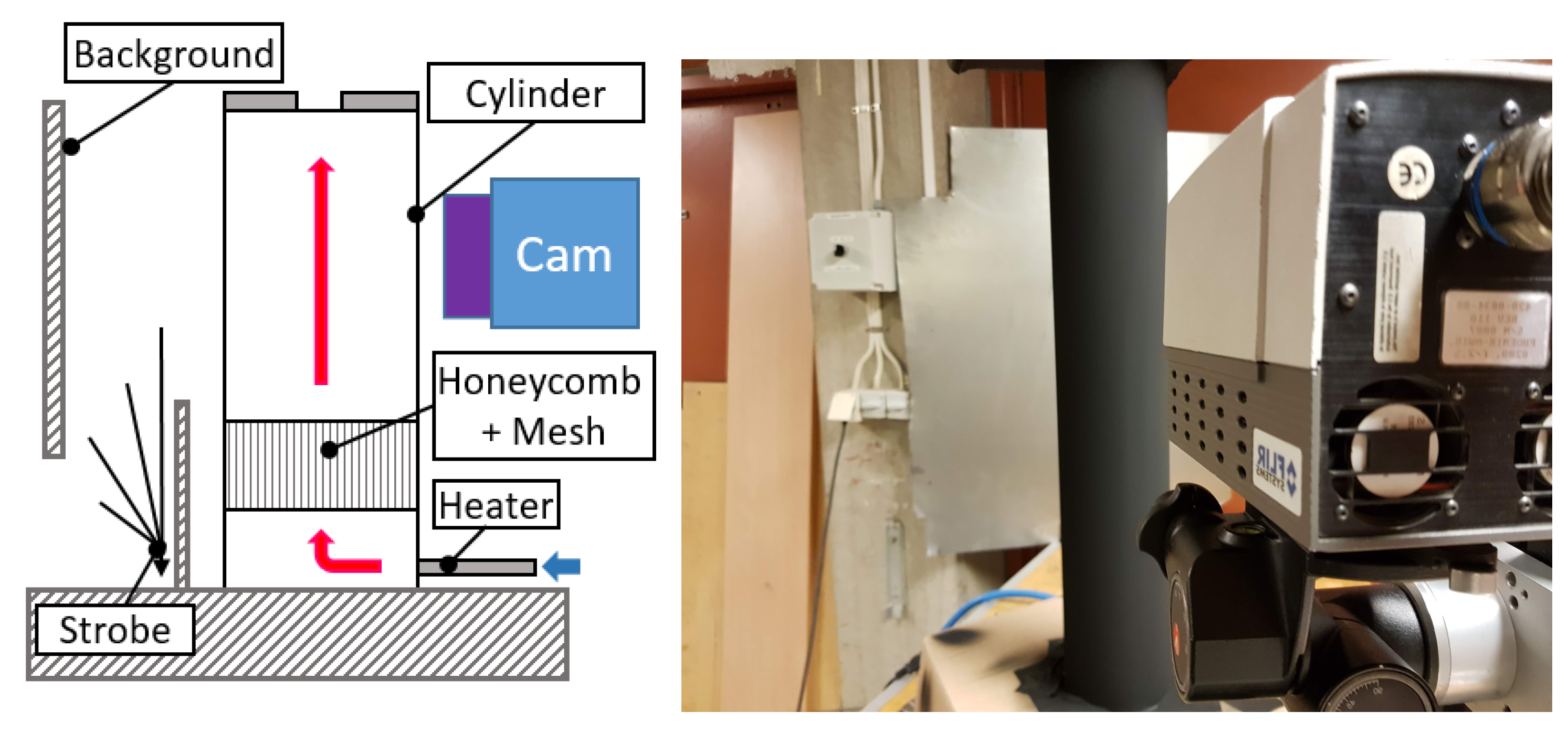
The in-house experiment was performed using a hollow heated aluminium cylinder which was coated with a Nextel 6081 coating and is shown in
Figure 7. The cylinder was placed vertically in a large cold and dark laboratory so the non-uniformity of the background radiation was negligible. To identify
the standard variation from a strobe light directed on the background was used. Two application methods of Nextel coating were tested, finely sprayed as applied on the OGV, and roughly applied with a brush.
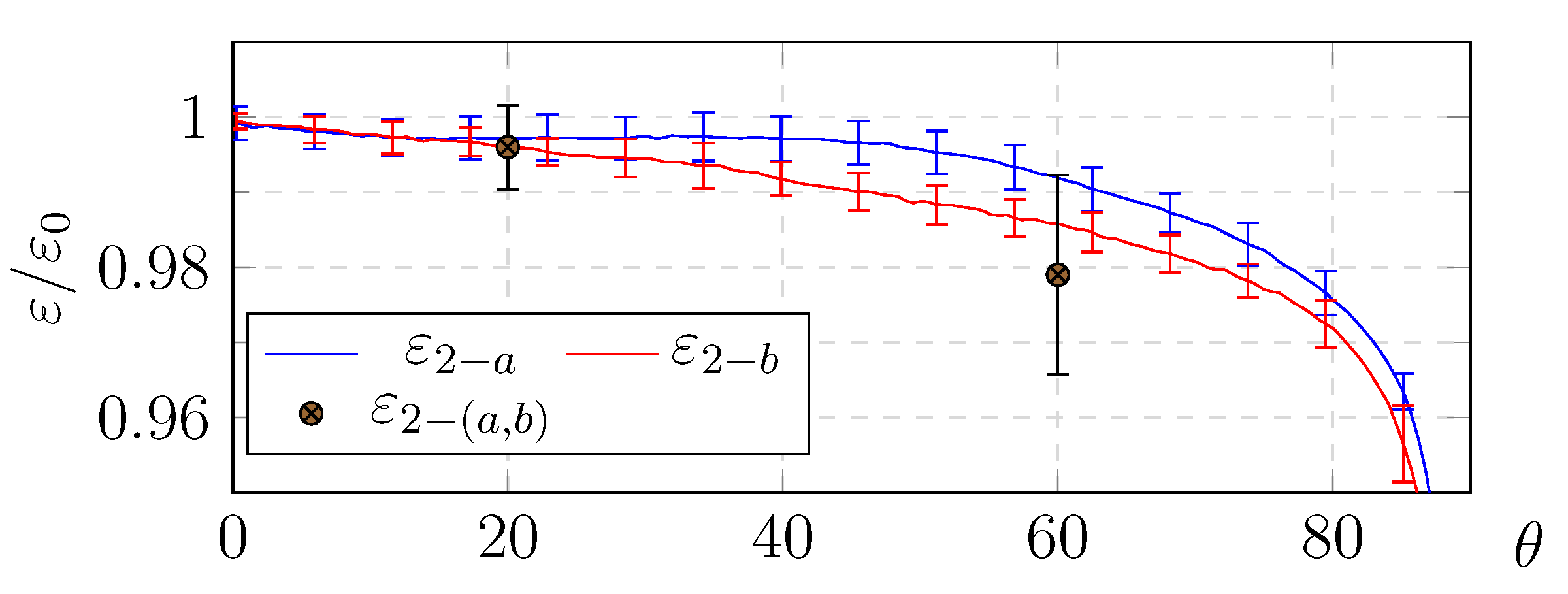
Figure 8 shows the angular dependence for spray (
) and brush (
) application. Values for
,
are based on 320 samples and the error bars depict two standard deviations along the length of the cylinder during calibration. The absolute value of the emissivity of both coatings was measured with an ET-100 thermal handheld emissometer at
at 20 and 60 degrees. The mean measured value is marked as
in
Figure 8 and the error bars show the full range of 10 samples from the handheld emissometer.
As shown in
Figure 8, the emissivity variation for
degrees is less than 1%, therefore only measurements at a view angle less than 55 degrees were used. This conservative threshold can potentially be extended if angular view correction is applied to the measurements. An ET-100 emissometer was used to measure the absolute emissivity of a gold leaf marker which was found to be
0.15 ± 0.1 at
20 and 60 degrees and is assumed to be valid for all
as well. The high variance in the emissivity of the gold leaf is believed to be due to contamination when adhered to the test geometry. The effect of this high variance have a relative small effect when performing a total error analysis.
4.7. Background Temperature
During the measurements, particular care was taken to account for the ambient radiation and reflections as these create a bias in surface temperature measurement. The RMA method first presented by Kirollos in [
7] provides a method to account for the background radiation using Equation (
9). The method assumes a similar temperature of the gold markers and the Nextel 6081 coating in the close vicinity. The perceived difference in temperature of the gold markers and the surrounding area is then used to isolate the background radiation since it provides two unknowns in a two-equation system.
is the effective background temperature and
is the wall temperature as defined in Equation (
1).
and
are the camera perceived temperatures on paint
and gold markers
respectively. The method requires a well-defined relative emissivity of both surfaces but is independent for absolute values. The gold leafs adhered to the relative rough OGV surface provides near-total diffusive reflection.
4.8. Radiative Heat Flux
To account for the radiative heat flux
the values
and
need to be defined, which is often an arduous task. However, it can be estimated using the calculated
from Equation (
9).
is the local effective background temperature from a surrounding black body and can replace
in Equation (
2) with
creating the expression
. Through using this method the radiative heat flux
was found to contribute with
for most of the OGV surface. Note that for surface temperatures in the test section, the radiative heat flux could be up to 3–10% of the total heat flux if the background were to be a complete black body, thus using the above correction is of great importance.
4.9. Three-Dimensional Effects and Post Processing
To accommodate for in lateral wall conductive heat flux a three-dimensional conjugate heat transfer was numerically simulated using FEM in both ANSYS™ and MATLAB™. The simulations were performed on a digital version of the test geometry’s shell by using
elements and normalised experimental data for core and surface temperature, later discussed in
Section 6. Some areas of the geometry’s surface could not be acquired by the camera due to geometrical limitations. Hence, to obtain a complete vane surface temperature for the FEM simulations, the nearest neighbour extrapolation was used. A conservative cut-off criterion has been applied to only use data where the wall thickness is uniform and far from the vicinity from the extrapolation. Because of this, data near the hub and shroud fillets and portions of the trailing edge have been removed. At areas with the highest surface temperature gradient, the effect from in-wall heat transfer when compared to the one-dimensional calculations is
. The uncertainties from the FEM calculation can be expected to be much smaller than this.
The surface view angle was calculated using the scalar product of the vector between the surface and camera lens and the surface normal vector. This was possible as the camera position was known and a digital twin of the experimental set-up exists. All view angles above 55 degrees were removed from the data set as variation in emissivity below 1% could not be guaranteed. The transformation from camera images to real-world coordinates onto the digital twin was achieved using the reflective markers as a reference for a linear interpolation of the image.
5. Summary of Measurement Uncertainties
In
Figure 9 the heat transfer coefficient
is shown along mid-span for the flow coefficient
. The shaded area shows the confidence interval of two standard variations, calculated using Equation (
3) with experimental data sampled during one camera view and uncertainties as stated in earlier sections. The confidence interval varies between 4% and 6% along mid-span as the contribution from different independent variable changes. For the whole full span data the calculated total uncertainty of the heat transfer coefficient
spans 2.5% to 8%. Two points are selected for detailed scrutiny and are marked in
Figure 9. The first, marked as A, is located at the minimum convective heat transfer at
. The second, marked as B, is located at
where the highest convective heat transfer occurs for that camera’s field of view (FOV).
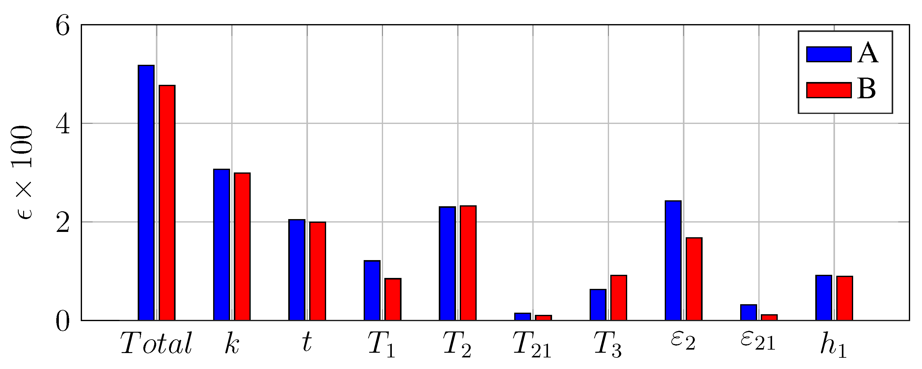
Figure 10 shows the uncertainty contribution and bias offset from individual variables at points A and B. The total uncertainty at point A and B is
and
respectively. For both points, the largest source of uncertainty is the thermal conductivity of the material but, as the heat transfer reduces, uncertainties in background radiation and radiative heat flux starts to have a larger contribution. Variable
in
Figure 10 is the bias offset from the inner wall heat transfer coefficient earlier discussed in the work. Note that the presented uncertainties are from a single data set and do not include errors from temperature normalisation or FEM calculations.
All aero-surfaces in the test section were geometrically verified using a ROMER absolute arm with an optical laser head with an accuracy of ±0.1 mm. The surface roughness was measured with Surtronic 3+ meter and was below 8 Ra.
6. Data Reduction
Before the different experimental data sets for the FEM calculations was merged, the one-dimensional surface heat transfer coefficient
was used to normalise the data. The one-dimensional heat transfer
was utilised together with nominal water
and air
temperature and Equation (
2) to provide the normalised surface temperatures
. The nominal temperatures
,
and
was then utilised as boundary conditions in the FEM simulation. As the variation in
and
could be kept small between different data sets, the radiative part could be neglected. This reduces Equation (
2) to a linear problem which is shown in Equation (
10).
7. Results
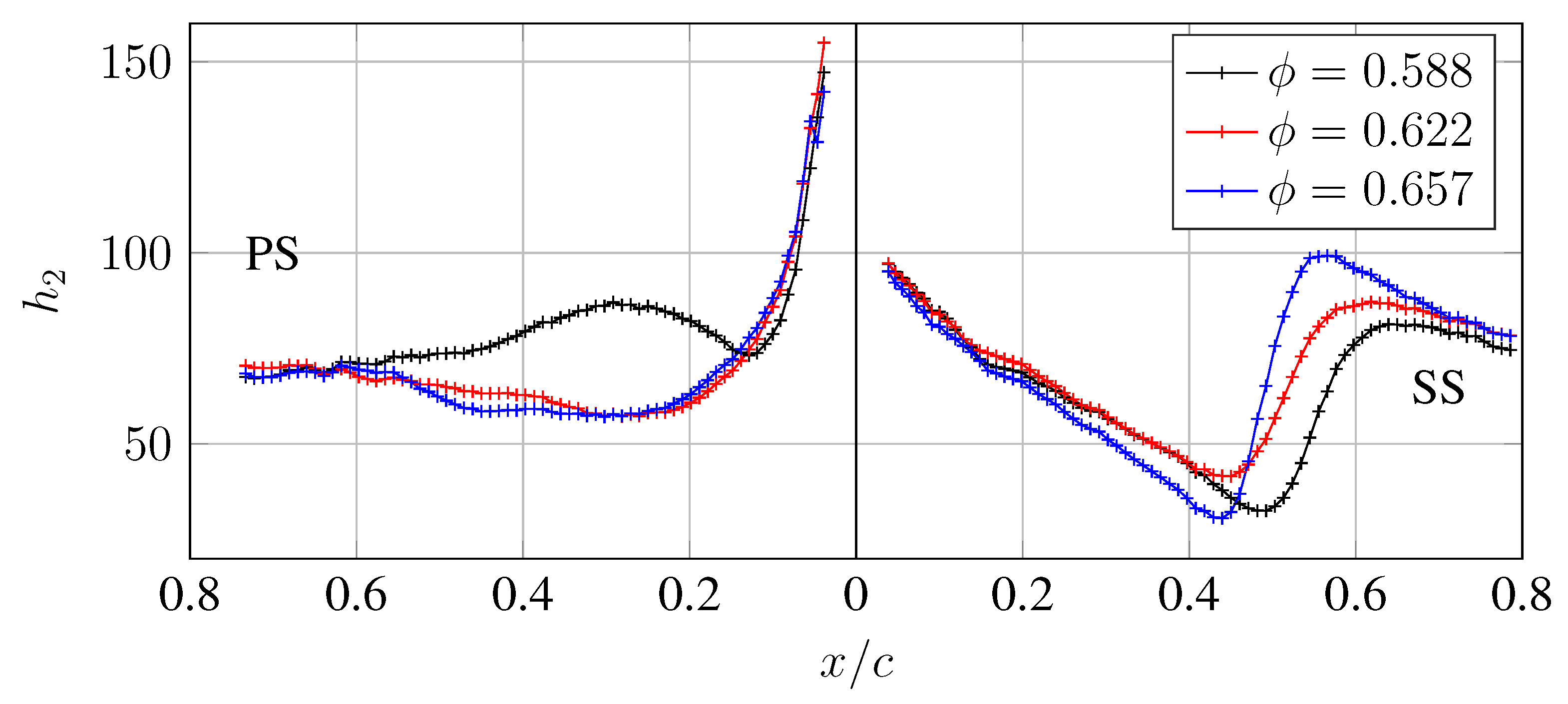
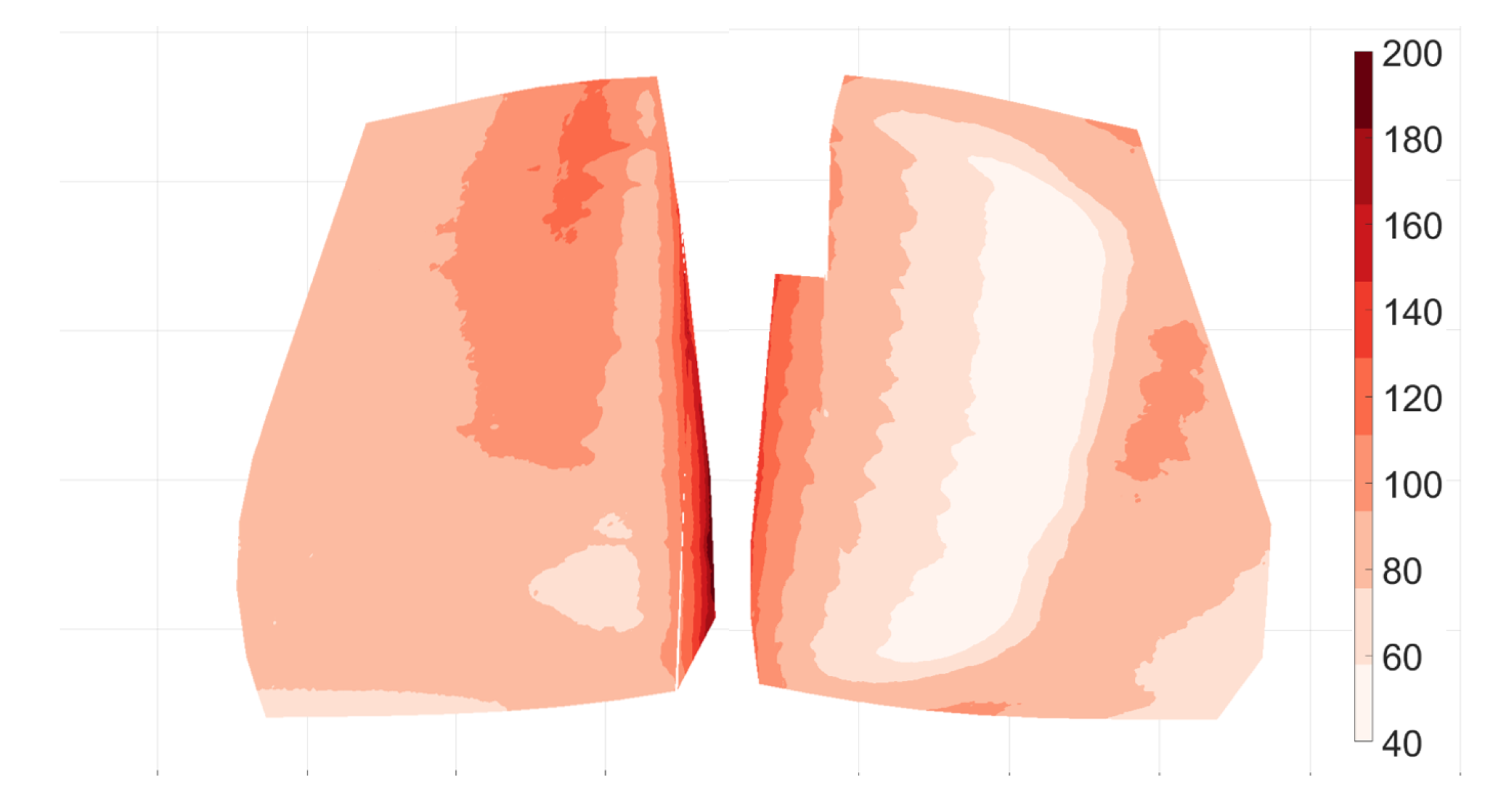
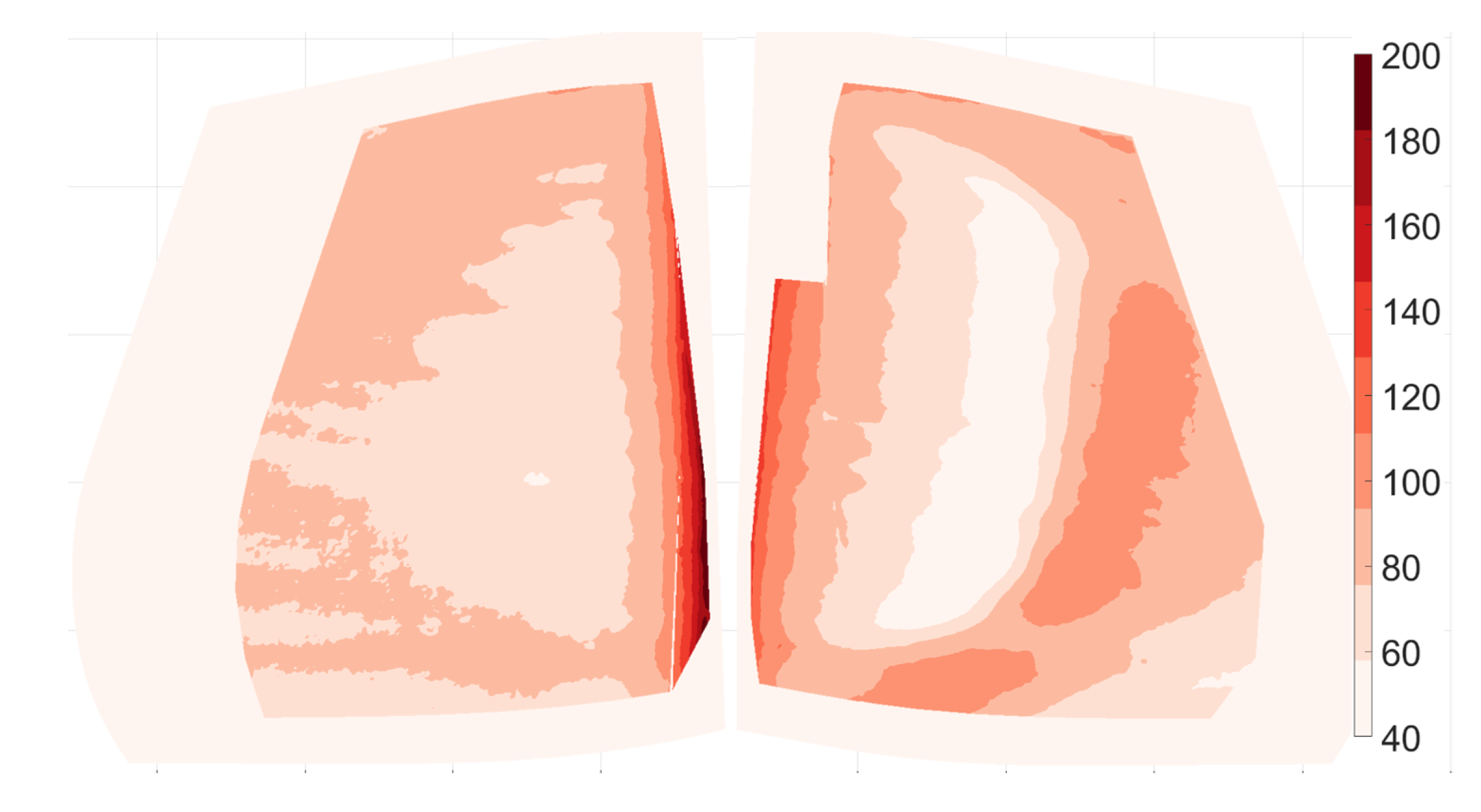
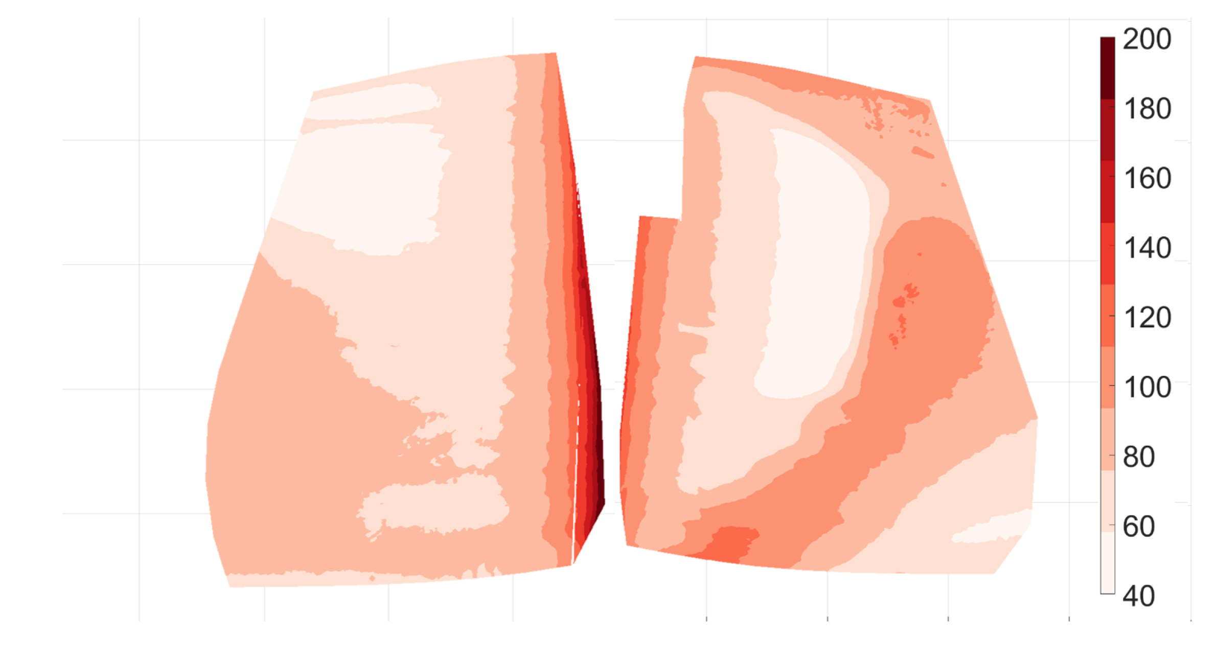
In
Figure 11 the heat transfer coefficient distribution is shown for three different aerodynamic loading conditions at Reynolds number 235000. For all cases, the heat transfer coefficient is largest at the leading edge and decreases as the boundary layer develops. For the suction side, a minimum is located at 45 to 55% chord followed by a steep increase for all the operating conditions. At the pressure side, the two higher flow coefficient
cases produces a very similar development while at the lowest inlet angle the rapid increase in heat transfer can be observed very early along the vane.
The steep increase in heat transfer is likely to be due to a laminar-turbulent transition. This is a commonly used rationale as skin friction is an order of magnitude higher in the turbulent boundary layer and hence by using the Reynolds analogy the heat transfer increases as well. The same rationale is adopted in the differential infrared thermography (DIT) measurement as used by Gardner in [
16] and by Filius in [
17]. Following this rationale,
Figure 11 shows a transition location moving upstream on the suction side with increased
. Note that an increased LPT flow coefficient
causes an increased inlet angle to the TRS and higher OGV blade loading. The two cases
and
show very similar trends. At
the change in heat transfer is larger in magnitude and shorter in length, indicating a different mode of transition. It is likely to be a bypass transition for
= 0.588–0.622 while a possible separation induced transition is occurring at
, the data in this work are however insufficient to state the exact nature of the transition. The steep increase of the HTC on the pressure side for the
case may be due to a separation induced laminar-turbulent transition as it only occurs at low inlet flow angles.
Data in
Figure 11 are based on four data sets and the merging and normalisation causes some minor bias offsets between them. At the suction side the two data sets are merged at
= 0.12–0.14 while at the pressure side it is at
. For the flow coefficient
an example of errors due to data merging can be seen as a cut in the data at the pressure side. The very few visible reference points and high curvature at this location make the geometrical data merging challenging and are believed to be the main reason for this. However, the observed variations are within the uncertainty of the measurement. Note that the values in
Figure 11 are not filtered.
Figure 12,
Figure 13 and
Figure 14 show the contours of surface heat transfer on the pressure and suction sides of the OGV at the different load cases. The data have been selected to comply to above-stated uncertainties, leading-edge data have been limited due to camera view angles over
, trailing edge, near hub and shroud data have been limited to keep uncertainties from FEM simulations to a minimum. The outline of the full vane is illustrated in
Figure 13. From heat transfer contours on the suctions side features such as roll-up vortex and transitions distribution can be deduced. The low heat transfer from the expanding roll-up vortex increases in effect spanwise with increased
. This has earlier been observed in [
10] (
Figure 7). Local points of high
can be seen near the hub for
; this area is a heavily loaded point with very high acceleration as earlier shown by pressure distribution in [
2], (Figure 4.15) and is an area of much interest for future studies.
8. Discussion and Conclusions
Experimental heat transfer investigations by infrared thermography (IRT) were successfully implemented on an outlet guide vane (OGV) in Chalmers LPT-OGV facility. Novel heat transfer measurements on an OGV in a TRS are presented at a range of flow parameters representing a set of engine conditions typical for throttle variation for mid-sized commercial engines. The full span heat transfer results indicate flow features such as laminar-turbulent transition and secondary flow structures but most importantly is the surface heat transfer itself. The full span surface heat transfer contributes to a more complete understanding of the flow in the TRS and thermal loads on the OGV.
Recently presented methods and modern manufacturing techniques was for the first time implemented in a holistic approach to minimise the uncertainty of convective heat transfer measurement. A detailed uncertainty analysis is presented for the heat transfer coefficient measurement which lead to an uncertainty of individual data points from to of reading. For the presented mid-span data, the uncertainty is in the range of to of reading. The presented method in this work has few geometrical limitations and can be implemented into a wide variety of applications. The authors identify the largest residual known uncertainty to be the material thermal conductivity and the reflective marker’s emissivity. The moisture and aging effect on the thermal conductivity of the wall material are estimated to be of high importance and should be further investigated. In the present study, the wall material was used during several weeks after manufacturing and was carefully dried after each experiment which lasted several hours. The authors want to point out that the heat transfer coefficient uncertainty presented in this work does not include error introduced from FEM calculations and data reduction.
Author Contributions
Conceptualization, I.J. and V.C.; Data curation, I.J.; Formal analysis, I.J. and R.D.; Funding acquisition, V.C.; Investigation, I.J. and R.D.; Methodology, I.J. and V.C.; Project administration, V.C.; Software, I.J.; Validation, I.J. and R.D.; Visualisation, I.J.; Writing—original draft, I.J.; Writing—review & editing, V.C. and R.D. All authors have read and agreed to the published version of the manuscript.
Funding
This research was funded by the joint research project AT3E as a part of the Swedish research programme NFFP-7 with grant number 2017-04861.
Acknowledgments
The support of GKN Aerospace Sweden, Chalmers Laboratory of Fluids and Thermal Sciences and to Loli Paz for ultrasound measurement is gratefully acknowledged.
Conflicts of Interest
The authors declare no conflict of interest. The funders had no role in the design of the study; in the collection, analyses, or interpretation of data; in the writing of the manuscript, or in the decision to publish the results.
References
- Rojo, B.; Kristmundsson, D.; Chernoray, V.; Arroyo, C.; Larsson, J. Facility for investigating the flow in a low pressure turbine exit structure. In Proceedings of the European Turbomachinery Conference, Madrid, Spain, 23–27 March 2015. [Google Scholar]
- Rojo, B. Aerothermal Experimental Investigation of LPT-OGVs. Ph.D. Thesis, Chalmers University of Technology, Gothenburg, Sweden, 2017. [Google Scholar]
- Arroyo Osso, C. Aerothermal Investigation of an Intermediate Turbine Duct. Ph.D. Thesis, Chalmers University of Technology, Gothenburg, Sweden, 2009. [Google Scholar]
- Rojo, B.; Chernoray, V.; Johansson, M.; Golubev, M. Experimental Heat Transfer Study in an Intermediate Turbine Duct. In Proceedings of the 49th AIAA/ASME/SAE/ASEE Joint Propulsion Conference, San Jose, CA, USA, 14–17 July 2013; p. 3622. [Google Scholar]
- Rojo, B.; Jimenez Sanchez, C.; Chernoray, V. Experimental heat transfer study of endwall in a linear cascade with IR thermography. EPJ Web Conf. 2014, 67, 02100. [Google Scholar] [CrossRef] [Green Version]
- Wang, C.L.; Luo, L.; Wang, L.; Sundén, B.; Chernoray, V.; Arroyo, C.; Abrahamsson, H. Experimental and numerical investigation of outlet guide vane and endwall heat transfer with various inlet flow angles. Int. J. Heat Mass Transf. 2016, 95, 355–367. [Google Scholar] [CrossRef]
- Kirollos, B.; Povey, T. High-accuracy infra-red thermography method using reflective marker arrays. Meas. Sci. Technol. 2017, 28, 095405. [Google Scholar] [CrossRef]
- Marcotte, F.; Tremblay, P.; Farley, V. Infrared camera NUC and calibration: Comparison of advanced methods. In Proceedings of the SPIE, Baltimore, MD, USA, 29 April–3 May 2013. [Google Scholar]
- Elfner, M.; Schulz, A.; Bauer, H.; Lehmann, K. A Novel Test Rig for Assessing Advanced Rotor Blade Cooling Concepts, Measurement Technique and First Results. In Proceedings of the ASME Turbo Expo, Charlotte, NC, USA, 26–30 June 2017. [Google Scholar]
- Jonsson, I.; Chernoray, V.; Rojo, B. Surface roughness impact on secondary flow and losses in a turbine exhaust casing. In Proceedings of the ASME Turbo Expo, Oslo, Norway, 11–15 June 2018. [Google Scholar]
- Industrial Platinum Resistance Thermometers and Platinum Temperature Sensors; Standard; International Electrotechnical Commission: Geneva, Switzerland, 2008.
- ASME. Test Uncertainty PTC 19.1.; Technical Report; ASME International ASME: New York, NY, USA, 2005. [Google Scholar]
- Plastics—Determination of Thermal Conductivity and Thermal Diffusivity—Part 2: Transient Plane Heat Source (Hot Disc) Method; Standard; International Organization for Standardization: Geneva, Switzerland, 2015.
- Vollmer, M.; Möllmann, K.P. Infrared Thermal Imaging: Fundamentals, Research and Applications; John Wiley & Sons: Hoboken, NJ, USA, 2010. [Google Scholar]
- Tang Kwor, E.; Matte, S. Emissivity measurements for Nextel velvet coating 811-21 between −36 ∘C and 82 ∘C. High Temp. High Press. 2001, 33, 551–556. [Google Scholar] [CrossRef]
- Gardner, A.D.; Eder, C.; Wolf, C.C.; Raffel, M. Analysis of differential infrared thermography for boundary layer transition detection. Exp. Fluids 2017, 58, 122. [Google Scholar] [CrossRef]
- Simon, B.; Filius, A.; Tropea, C.; Grundmann, S. IR thermography for dynamic detection of laminar-turbulent transition. Exp. Fluids 2016, 57, 93. [Google Scholar] [CrossRef]
© 2020 by the authors. Licensee MDPI, Basel, Switzerland. This article is an open access article distributed under the terms and conditions of the Creative Commons Attribution (CC BY-NC-ND) license (https://creativecommons.org/licenses/by-nc-nd/4.0/).


