1. Introduction
Development of gas turbine engines is a highly iterative procedure that involves different disciplines [
1]. The first step in the development of a new engine is the preliminary design phase, where different concepts and configurations are assessed at design and off-design, steady-state and transient conditions, for identifying the optimum one that fulfills the respective performance and installation requirements. The choice is guided by seeking optimality, while not violating a number of performance, aerodynamic, structural, and installation constraints. Of all engine components, the compressor is probably the most important and critical one due to the flow physics involved. A good compressor design is essential for achieving the desired performance and operating range. Performance at a wide range of operating conditions has thus to be accurately evaluated and accounted for, as early as possible during the design of a new engine.
During the early design stages, the need for fast and reliable multi-fidelity and multi-disciplinary platforms (e.g., [
2,
3]), has made compressor mean-line (1D) models a valuable tool for the designer. They allow studying the effects of heat transfer [
4], water evaporation, novel combustion concepts [
5], and low-power operation on compressor aerodynamics [
6]. In contrast to higher fidelity tools [such as 2D or fully 3D Computational Fluid Dynamics (CFD) codes], 1D tools are fast, have acceptable accuracy if appropriately tuned [
5], need only a few geometry inputs, and don’t need an expert user to set-up the model and calculation case. They allow designers to easily capture compressor performance trends and evaluate the effect of compressor aerodynamics on overall engine performance. For this reason, although they first appeared a long time ago, they remain of current interest and are the subject of research efforts today (e.g., [
5,
6,
7]).
Mean-line codes use physically consistent modelling to capture compressor flow physics and predict performance at different conditions, using correlations and high-level indices of blade row performance. The nature of the equations they use leads to convergence problems, when the compressor works at or beyond choking conditions. Even modern 1D codes employing the approach introduced long ago, for instance in [
8], still use a “pre-processing” step for determining the useful operating range “manually”. The inlet mass flow rate changes incrementally until the code producing a compressor map fails to converge as the inlet mass flow approaches or reaches the choking value. One such example is a NASA code named “OTAC” (Object-oriented Turbomachinery Analysis Code) [
9,
10], that conducts mean-line or stream-line design and off-design performance calculations, for radial- or axial-flow turbomachines. For a speed-line, the flow where one (or more) compressor blade rows choke is taken equal to the value for which the code fails to converge [
10]. In another code for compressor mean-line calculations, also developed at NASA [
11], the working mass flow range is determined iteratively by varying the incidence angle of the first rotor row and for any given speed the maximum flow is identified when the code fails to converge.
Attempts to modify the set of mean-line equations so that turbomachinery performance models can work without convergence problems within the choked portion of the map have been demonstrated successfully only on multi-stage turbines [
12]. Because of the more complicated nature of the flow involved, the real challenge in modelling compressor choke “lies primarily in understanding the mechanisms causing it”, as stated by Hendricks in [
12]. In that direction, various efforts were made to model compressor choking. Arolla et al. [
13] described a low-order approach for modelling the blade row throat passage choke for subsonic and supersonic inlet conditions. They also proposed a method for producing the vertical portion on the characteristics map, by introducing additional losses at the last choked blade row until the compressor back pressure was attained or a downstream blade row choked. They demonstrated successfully the application of their method on a single-stage fan. Cadrecha et al. [
14], used simple flow equations to first identify the conditions (in terms of flow Mach number) that lead blade rows and ducts to choke. They then formulated a bisection method for solving the system of mean-line equations at subsonic, supersonic, and choke conditions. They also described a modelling approach for extending the choked portion of the map characteristics where they increased the losses of the duct following a choked blade row, until the last row or the compressor exit chokes. The proposed methods were exemplified on a “dummy” geometrical model of a multi-stage turbine with zero losses and demonstrated for the case of a single-stage compressor for which a performance map was produced for three rotational speeds.
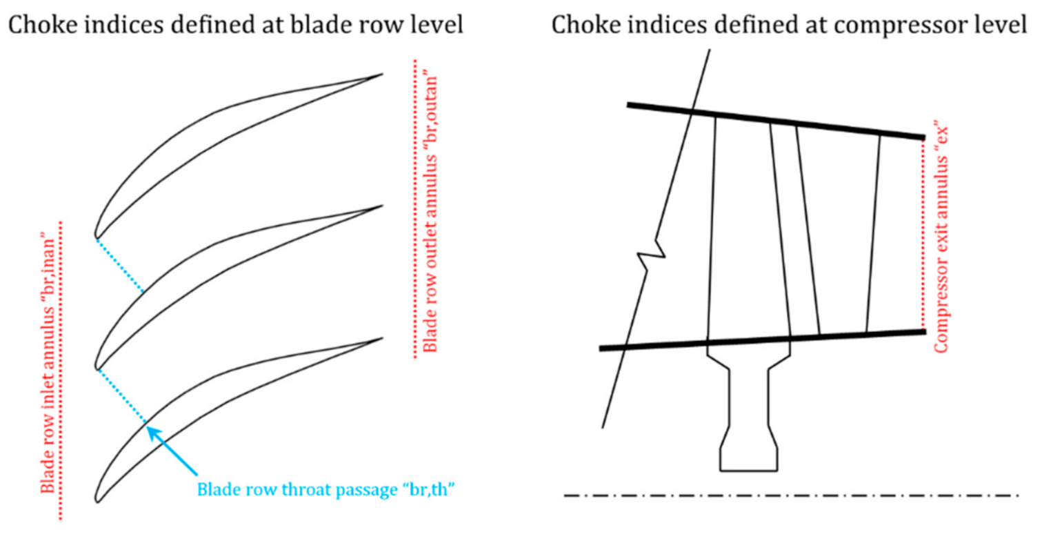
In the present paper, a Mean-Line Code (MLC) is developed that combines and extends the modelling approaches of [
13,
14] for choke modelling. Choke is examined by considering both throat and flow annulus (in [
13,
14] the one or the other alone is considered). Appropriate indices are introduced to quantify how far any blade row or annulus operates from choke. The maximum flow the compressor can deliver is established by zeroing these indices using a robust numerical procedure. Overall, a physically consistent, transparent, and fully automated procedure is proposed, for producing the entire compressor performance map. For the first time in the open literature, multi-stage compressor maps are generated with inter-stage flow features captured in the full operating range, including the “vertical” part of the characteristics.
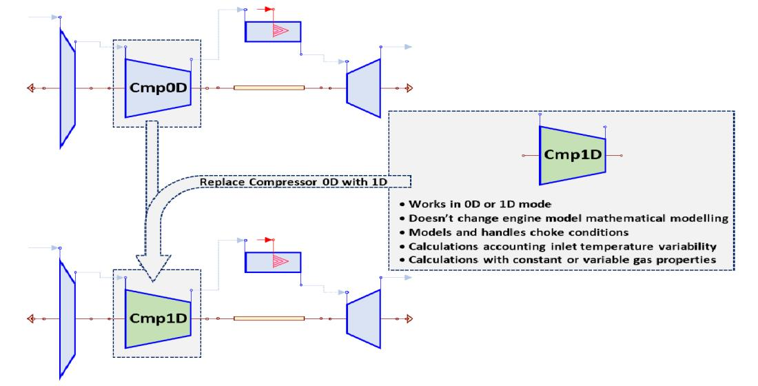
The developed MLC can be integrated in an overall gas turbine engine model, replacing the traditional performance maps. Such a replacement offers possibilities for more accurately representing overall engine performance, while it provides additional flexibilities for handling effects that are very cumbersome to introduce when legacy maps are employed. Example effects of this type are map variability versus inlet temperature, variable geometry, variable inter-stage bleeds, water ingestion or inter-stage injection, incorporation of heat transfer effects at stage level.
Although mean line codes have been presented in the public literature, there are no cases where such a code is developed, integrated, and used for simulation in a 0D cycle analysis in a consistent, transparent and robust way similar to that of conventional 0D components. Typically, 0D and 1D codes are developed independently of each other (sometimes using different programming languages, gas caloric properties, solvers, etc.), which results in thermodynamic and numerical inconsistencies between them. NASA’s code OTAC [
9,
10] is an exception to this, but up to now there has been no publication demonstrating its coupling with an engine model. Generally, there are three approaches for coupling the 1D (or higher fidelity) and 0D cycle analysis codes [
15,
16]:
De-coupled: the higher fidelity code is used to generate compressor characteristics which are then used as data in the conventional 0D cycle code (e.g., [
3]).
Semi-coupled: An iterative scheme is implemented, where the 0D cycle analysis provides boundary conditions to the 1D code and then the 0D component performance is updated according to the higher fidelity results. This loop is repeated until 0D and 1D performance is matched within a user-defined tolerance (e.g., [
17]).
Fully-coupled: The higher fidelity component is fully integrated in the cycle analysis (e.g., as an external object) directly replacing the corresponding 0D component [
18].
In the de-coupled approach, the mathematical formulation of the 0D cycle analysis is not affected, but the map is valid for the geometry and secondary effects (bleed-off takes, inlet temperature, heat transfer, water injection/ingestion) for which the map is generated, while map interpolation reduces accuracy. Semi- or fully-coupled approaches necessitate a change in the mathematical formulation of the conventional cycle model and/or the model building logic, which can affect simulation robustness. The exchange of information between the codes impacts speed of execution. In the fully-coupled approach, map interpolation is not needed, avoiding thus accuracy compromise.
A versatile fully-coupled approach for integrating a mean-line code in an engine model is proposed in the present paper. A 1D code is developed as a stand-alone component in the same environment as 0D components and uses the same interface and functions for numerical, working fluid model and thermodynamic calculations. This ensures modelling homogeneity and mathematical robustness during mixed-fidelity calculations while facilitating code extendibility and maintainability. The component can operate either as 0D or 1D, preserving the mathematical formulation of existing 0D performance calculations and handling choking at component and engine level, and accounts for changes in geometry and bleed off-takes. Gas modelling with either variable or constant gas properties can be selected, if execution speed up is needed, e.g., during optimization and design space exploration studies.
The implementation is exemplified through steady state and transient simulations of a turbofan model at both altitude and sea-level conditions where the component is used as the high-pressure compressor (HPC), for both 0D and 1D modes.
In the following, the 1D modelling and the methodology for modeling compressor choking and generating the map are first presented, followed by the description of how the component produced is integrated in an engine level.
2. Mean-Line Code (MLC)
The Mean-Line Code for performance analysis of axial-flow, multi-row compressors, was developed and validated in the same environment as the conventional 0D components for turbomachinery performance simulations, used to build overall engine models. The environment used was the Propulsion Object Oriented SImulation Software (PROOSIS) with its TURBO library [
19,
20]. Existing 0D compressor components were extended to add the 1D capability. The new component developed inherites the same fluid and mechanical interfaces to enable interconnections with other components and/or systems, and the same functions for numerical, fluid flow, and thermodynamic properties calculations. A transparent integration in engine cycle analysis calculations, without affecting the mathematical formulation and the simulation robustness, is thus ensured. A brief description of the 1D modelling is given below.
For known compressor geometry [i.e., flow annulus hub and tip radii, basic dimensions of blades and blade metal angles at leading (LE) and trailing edges (TE)], inlet flow conditions (, , ), and compressor speed (), the MLC calculates the compressor exit total pressure and temperature by conducting a row-by-row calculation, applying loss and deviation models for individual blade rows. The building blocks of MLC are the Blade Row Module (BRM) modelling individual blade rows, and the Inter-Volume Module (IVM), modelling the duct after a blade row.
In the IVM, gas bleeds are applied through mass and gas composition continuity, annulus radius changes are taken into account through a moment of momentum balance, while heat transfer, water-vapor injection (i.e., gas mixing), and pressure loss effects have also been foreseen. BRM models any type of blade row [rotor, stator, inlet guide vanes (IGVs), of variable or fixed geometry] and establishes the row outlet conditions by solving iteratively the set of equations formed by mass and gas composition continuity, the conservation of energy, and loss and deviation correlations introduced to calculate the flow across the row. More specifically, the aerodynamic performance of diffusing rows is modelled in terms of Lieblein’s diffusion and equivalent diffusion factors [
21], where the design incidence and deviation angles are calculated using Herrig’s and Lieblein’s correlations [
21], respectively. The blade row deviation angle (
) and, thus, outlet flow angle, is estimated using Swan’s model [
22]. Across a row, the Euler pump equation for rotors or the conservation of total enthalpy for stators gives the outlet total enthalpy, while the exit total pressure is estimated using a total pressure loss coefficient (
). In
, profile, secondary, and endwall losses are accounted for according to Aungier [
21], clearance losses are modelled using the simplified model of Lakshminarayana [
23], shock losses are calculated according to Steinke’s shock model [
24], while Mach and Reynolds number effects are taken into account following Aungier [
21] and Koch et al. [
25], respectively. For IGVs,
and
are calculated according to Banjac et al. [
26]. The loss and deviation models used in MLC are fully tunable through appropriate scalars, the value of which can either be the default one, a user input, or evaluated numerically. The code is also fully scalable, in the sense that the user can switch on or off any of the above loss sources, and can easily introduce customized loss and deviation models. A summary of the default loss and deviation correlations mentioned above can be found in
Appendix A.
Finally, the code has the possibility to perform calculations with variable or constant gas properties for each blade row. In the latter case, specific heats ratio (
) and specific heat capacity (
for a blade row, are calculated based on appropriate local temperatures. It was found that the results of such calculations are very close to those of using the full gas model when the blade row inlet temperature for stators, and average inlet-outlet temperatures for rotors
, is employed. The local temperature at any station along the compressor is evaluated by assuming that each stage,
, achieves the same temperature rise
, which is given by the following formula:
assuming a polytropic efficiency of
,
, and the compressor design pressure ratio value as the average total pressure ratio
. Only the thermodynamic properties are calculated using the local
and
, instead of using the full expressions of fluid and thermodynamic models that calculate gas properties as function of temperature and gas composition. The magnitude of differences of the results using the two approaches will be presented in the results section.
4. 1D Component Model for Integration in 0D Cycle Analysis
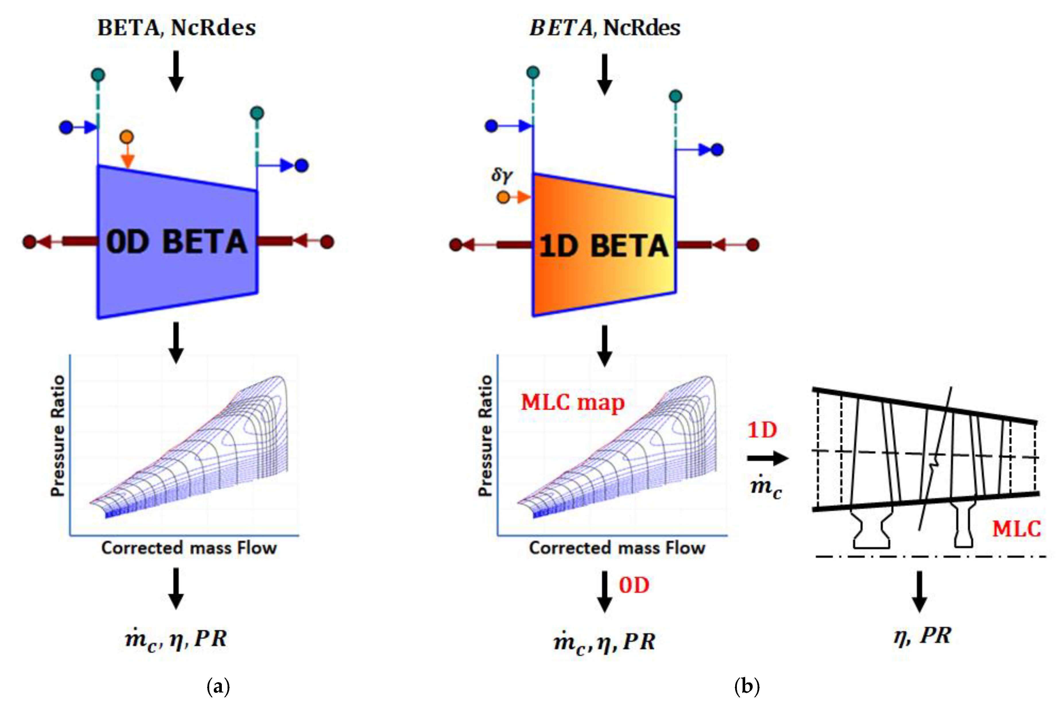
In its simplest form, a conventional 0D compressor component (
Figure 3a) establishes performance by reading a set of tables (a map) that return corrected mass flow rate (
), isentropic efficiency (
) and pressure ratio (
) for given values of the auxiliary map parameter (BETA) [
29] and corrected speed relative to design (NcRdes). BETA is an independent (or algebraic) variable at engine model level that the numerical solver (e.g., Newton-Raphson) adjusts in order to ensure consistent operation of engine components [
30].
MLC, on the other hand, requires mass flow rate
and compressor speed
as inputs and returns
and
. For this reason, the new component implements a two-step, hybrid approach, enabling it to be used in either 1D or 0D mode (user-defined option), while also maintaining the traditional 0D algorithmic logic when the 1D mode is employed. This requires the use of a map that is generated with the MLC through a dedicated simulation case using the modelling approach described above. This is a necessary pre-processing step before the component can be used. Actually, a multitude of maps are generated for a range of compressor inlet temperatures
[including of course the International Standard Atmosphere (ISA) conditions] in an effort to improve calculation accuracy (irrespective of operating mode) since conventional gamma corrections [note that, typically a map is generated for a given compressor inlet temperature (e.g., at ISA conditions) and gamma corrections are applied to account for the effects of different temperatures during simulation] arenot sufficient [
31]. Then, when the component workes in 1D mode, BETA is still used as an algebraic variable for reading the map of the pre-processing step to obtain a mass flow rate value
. Next, this
value is used to execute the MLC and derive the compressor performance (
Figure 3b). The MLC-generated map provides the required
–BETA relationship, which otherwise would have to be established through multiple MLC executions during every cycle calculation. Furthermore, the map acts as a reference in order to correctly account for the current operating conditions, as will be explained in the following.
During the pre-processing step, a table is also derived with the values of BETA (BETAchoke) below which choking occurs. The independent variables for reading this table are compressor corrected speed NcRdes and . So, when the component operates in the 1D mode, the current value of BETA is compared with BETAchoke to determine if operation is in the choked region or not.
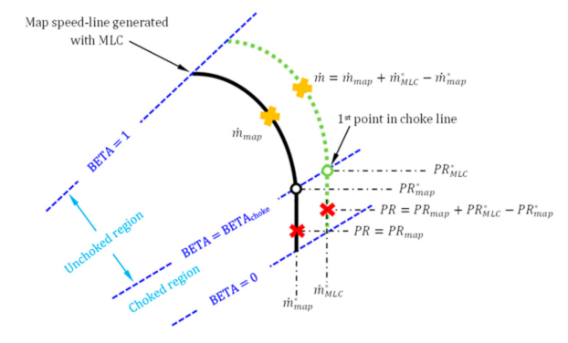
If unchoked, the value of mass flow rate is obtained from the map (
) for the current BETA, NcRdes, and
. To account for changes between 1D performance for the current compressor operating conditions and map (generated for some reference conditions), the 1D code is executed once to find the first point in the choke line (
) for the current conditions (see
Figure 4). A correction is then performed in the value of mass flow
for which the 1D code is executed in the unchoked part to account for any shift (
) in the position of the choke line (compared to map value
).
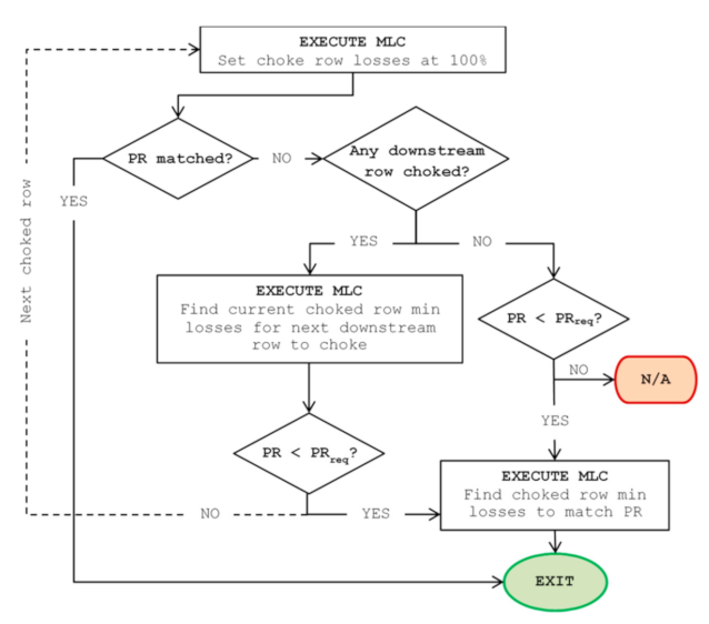
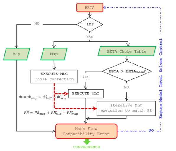
On the other hand, if BETA < BETA
choke, the logic presented in
Figure 2 is implemented, where for
, the required
is the one obtained from the map, but corrected for the current compressor operating conditions, as illustrated in
Figure 4. The algorithm establishes the choked row losses that will result to the required compressor exit pressure. The complete algorithmic logic of the new 0D/1D component is depicted in the flowchart of
Figure 5.
5. Example Compressor Map Results
The MLC choke modelling and the 1D model integration capabilities are exemplified using the geometries of two multi-stage compressors, NASA’s ISG-74A [
32] and NASA/GE’s E
3 HPC [
33]. NASA’s ISG-74A is a 3-stage transonic, high-speed compressor developed and tested during the 80s, while NASA/GE’s E
3 HPC is a 10-stage transonic, high-speed, high-aerodynamic loading compressor developed and tested during the late 70s-early 80s. Basic geometry and performance details for both compressors are summarized in
Table 1.
Note that the default loss and deviation models used in MLC were mostly developed on the basis of cascade tests in subsonic wind-tunnels during the early 50s and, hence, they cannot capture the performance of current transonic compressors, as explained in [
5]. MLC offers the capability of calibrating numerically these models for representing current compressor aerodynamics. An example of reproducing a compressor map through such a calibration is given in
Figure 6 for NASA’s “Stage-35” [
34]. Thus, it is shown that the method proposed contains the flexibility to adapt to and correctly model the performance of axial compressors. We will not further discuss this aspect of the method, since the focus of the present work is to discuss the features of the process for establishing choked operation and its integration in engine models. Therefore, the geometries of the compressor test cases used serve merely as a demonstration of the capabilities developed and not for validating MLC against publicly available data. In what follows, MLC is executed with its default loss and deviation models.
5.1. Choke Modelling
Choke modelling capability is demonstrated on the geometry of a 3-stage transonic compressor [
32], see
Table 1. For easy reference in the discussion, the following designation is used for the compressor blade rows: IGV-R1-S1-R2-S2-R3-S3, where “R” stands for rotors and “S” is for stators.
The map produced by the MLC is shown in
Figure 7. It was produced for standard-day conditions, assuming axial flow at the compressor inlet, zero bleed extractions, at the design IGVs-stators setting. The choked mass flow rate was calculated using a value of
in Equation (7), while a lower bound on the total pressure ratio of
was imposed when establishing both the first and the last point on the choked portion of the map characteristics. Between stall and choke,
was calculated for 11 equally distributed values of
along each speed-line.
The lines that connect the respective first and last choke points on every speed-line are also presented in
Figure 7, defining the domain where the compressor operates at the maximum inlet mass flow. For
and 30% the maximum flow is established from the limiting pressure ratio value of
and, therefore, no vertical portion of the characteristics exists. The compressor works unchoked at these two speeds. Numerically, this means that the secant method cannot zero the functional expressed in Equation (7) for the value of
while satisfying the constraint
. At both these points,
has the minimum value which is about two orders of magnitude greater than the value of
for which choking is assumed to numerically occur. For
, there is a narrow region on the map characteristic where the compressor can work at the maximum mass flow. Here, the compressor chokes for the first time at the throat of S3, while the last choke point is established from the constraint
which is met before the compressor exit annulus becomes choked.
Table 2 summarizes the rows and stations where the first and last choke points occur for the speed-lines with
.
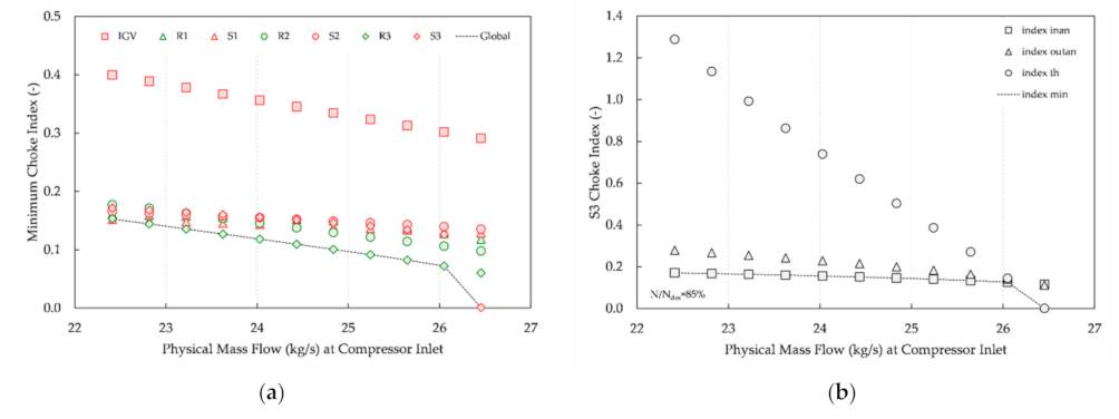
To illustrate in more detail how the first choke point is established numerically, the
speed-line is used as an example. In
Figure 8, the choke indices values are plotted against
as it increases towards the choking value.
Figure 8a shows the variation of the global minimum index
) and the variation of the minimum blade row index
) for all blade rows, while
Figure 8b shows the variation of the individual S3 indices,
,
,
, and
.
From
Figure 8a, it is seen that
for
between 22 and 26 kg/s, while in the same mass flow range the distance between
and the values of all other indices either increases or remains constant as
increases. This means that, if the compressor were to choke for a
value between 22 and 26 kg/s, it would be due to R3 becoming choked. As, however,
approaches the choking value (
kg/s),
experiences an abrupt value drop and becomes less than
. This in turn results in an abrupt drop in the value of
, causing the compressor to eventually choke for the first time at S3 as its value becomes equal to that of
. The reason for the drop in
value can be found in
Figure 8b. It is observed that
for
between 22 and 26 kg/s and, using the same rationale as before, if S3 were to choke for a
in this range it would be due to the choking of the row inlet flow annulus. However, the distance between
and the other indices decreases as the mass flow increases and, for a
value slightly greater than 26 kg/s the difference between
and
finally becomes negative, therefore causing the drop in
value and S3 to choke at the passage throat instead as
approaches the choking value.
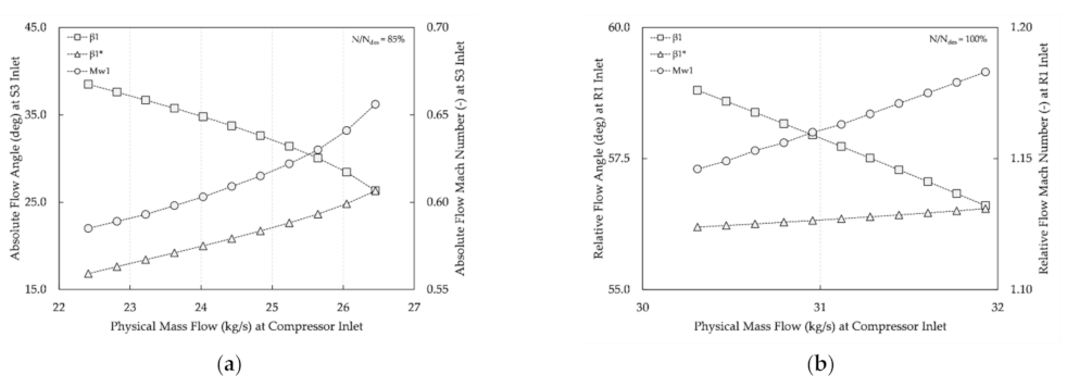
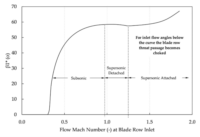
The absolute flow Mach number at S3 inlet is shown to be subsonic, for all
kg/s, in
Figure 9a. As the flow Mach number increases, the minimum flow angle required for the throat to become choked (
) increases as well, while the absolute flow angle at the inlet of S3 decreases until the two become equal within the specified tolerance of
and, therefore, the throat passage choking for S3 is realized for subsonic conditions. This is in contrast, for instance, to the R1 throat passage choking for
where, as seen from
Figure 9b, the relative flow Mach number at R1 inlet is supersonic for
kg/s and the throat passage chokes for supersonic conditions with attached shocks.
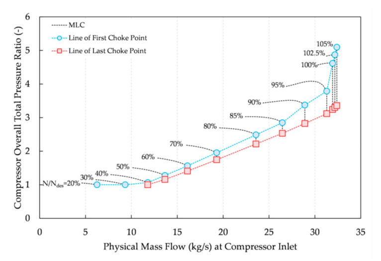
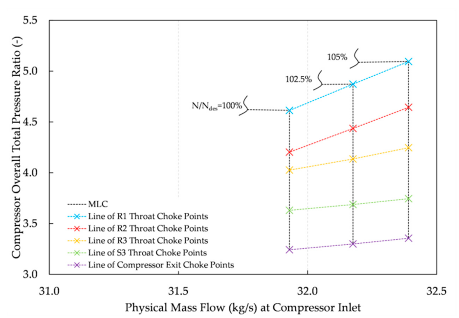
Τhe method to extend the choked part described in
Section 3.3 is exemplified considering the speed-lines 100%, 102.5%, and 105%. In all three speed-lines, both the first and last choke points occurred at the throat passage of R1 and the compressor exit, respectively. Thus, these speed-lines were a good example for viewing how the choke point moves from R1 (almost at the compressor inlet) until it reaches the compressor exit flow annulus.
Figure 10 shows the outcome of the procedure of the flow chart in
Figure 2. It shows the “iso-choke” lines that denote the different rows and stations that choke successively as the compressor
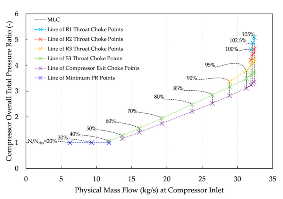
is reduced. It is shown that choking advances from R1 to R2 to R3 to S3 until the compressor exit is reached and the minimum pressure ratio for which the compressor can work is attained. For all blade rows, choking occurred at the respective throat passage. For all three rotors, the flow regime at the respective inlet is supersonic with attached shocks, while the flow at S3 inlet is subsonic. An overall pressure ratio map showing the “iso-choke” lines for the case of the example 3-stage compressor geometry is presented in
Figure 11.
5.2. Example of MLC Integration in Engine Model
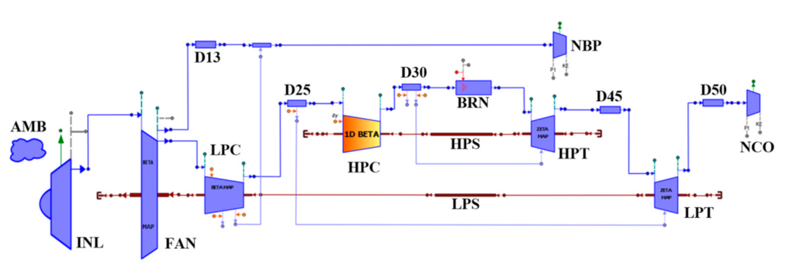
For demonstrating the integration and simulation of the newly developed 0D/1D component in an engine performance model, the case of a two-spool, unmixed flow turbofan engine was considered where the component is used for the HPC. Since the fluid and mechanical interface of the component in hand is identical to the corresponding 0D one, it can be connected to other relevant 0D components without any changes in the model building procedure, as shown in the schematic diagram of
Figure 12.
Similarly, the mathematical formulation of this mixed-fidelity engine model is identical to the conventional 0D performance case, in terms of boundary conditions (only one handle variable was required, e.g., thrust or fuel flow rate), algebraic (turbomachinery component map parameters, bypass ratio, inlet mass flow rate) and dynamic (low and high pressure spool rotational speeds) variables.
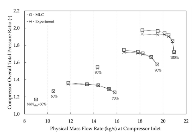
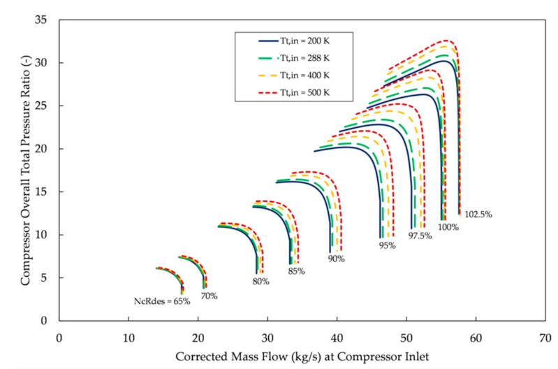
The 1D component was set to represent the NASA/GE E
3 HPC as far as the necessary stage, blade, and geometric input data required [
33]. Following the pre-processing step, a map (
Figure 13) is generated for four compressor inlet temperatures, covering the expected range for the considered application (
200, 288, 400, and 500 K). In fact the map is a set of 3D tables describing
,
and
in terms of BETA, NcRdes, and
. In addition, the table of BETA for each corrected speed below which choking occurs is produced (0.20 < BETA
choke < 0.27).
An engine design calculation was performed first in order to calculate at cruise conditions (
m,
) the scaling factors for the 0D map components [fan, booster, high- (HP) and low-pressure (LP) turbines] and the throat areas of the convergent bypass and core nozzles. The boundary variables in this calculation include the location of the design point on the maps of the 0D map components, their polytropic efficiencies, the pressure ratio values of the fan (bypass and core) and booster, the bypass ratio, the LP spool rotational speed, and the turbine inlet temperature. To obtain a valid operating point for the HPC, BETA and relative corrected speed were specified (in analogy to specifying the design point on the 0D map component). The values of the main engine cycle parameters are included in
Table 3.
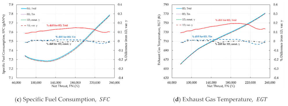
Off design simulations were then performed to generate a steady-state operating line and a transient square cycle between low and high power conditions at both altitude ( m) and Sea-Level Static (SLS) conditions. Simulations are performed in both 0D and 1D mode for the HPC component and in the latter case, for either variable or constant gas properties. For simulations with constant and , an overall total pressure ratio value was assumed equal to the HPC of the previous calculated point.
Figure 14 shows the variation of selected HPC and engine parameters with thrust (control parameter) at SLS conditions, for four simulation options, presented in order of increasing computational complexity:
- 1.
0D mode using single MLC-generated map at standard temperature of K.
- 2.
0D mode using MLC-generated maps according to actual HPC inlet temperature
- 3.
1D mode with constant
- 4.
1D mode with variable gas properties
As the differences were small compared to the range of variation, the percentage difference of results from each of the first three cases from the last one is also shown.
As expected, the first option (0D map with single map) shows the largest differences (up to −0.35%) from the 1D mode with variable gas properties. The other two are well within ±0.1% (±0.05% for the 1D mode with constant γ). The use of 0D mode with as an extra dimension shows the importance of obtaining the compressor performance for the actual inlet conditions and justifies the need for the 1D mode, since otherwise the 0D mode would require the generation and use of multi-dimensional tables/maps, where all possible combinations of compressor operation are included (variable geometry, bleeds, evaporation, etc.). Finally, the use of the 1D mode with constant γ proves to be an acceptable surrogate of the mode with variable gas properties, as it does not compromise the accuracy of calculations while it executes much faster. In our calculation, it was approximately 45% faster compared to the MLC with variable gas properties and in a desktop PC (Windows 10 Pro 64-bit, Intel® CoreTM2 Duo CPU at 3GHz with 8GB RAM) required less than 5 s for a complete engine simulation to converge to a tolerance of less than 10−6. In comparison, the 0D mode executes in less than 0.05 s.
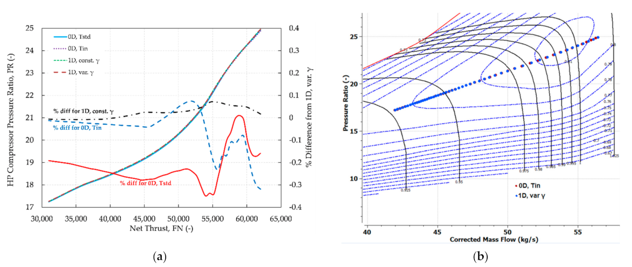
Repeating the same simulations at flying altitude (
m,
), similar levels of differences were observed between the different modes, as for the SLS simulations. This is demonstrated in
Figure 15a for the HPC pressure ratio. However, at these conditions, there are operating points in the region of the map where the corrected speed iso-lines are almost vertical,
Figure 15b. As a result, map interpolation causes a fluctuating variation of differences between 0D and 1D modes in this region. Furthermore, it is in this region that the mass flow rate correction presented in
Figure 4 makes the MLC execution possible since otherwise even a small difference in mass flow rate can produce a value that is outside the working range of the 1D code.
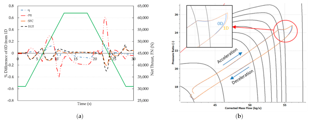
Transient simulations at flight and SLS conditions produce similar results to the steady state ones, with differences again being slightly larger at altitude. The variation with time of the differences between the 0D (using
) and 1D (variable properties) modes for selected compressor and engine parameters is shown in
Figure 16a for cruise conditions. The differences show peaks during the acceleration and deceleration parts of the simulation, which is again attributed to map interpolation, especially since in the latter case the operating line is in the region of the map where the speed iso-lines are almost vertical,
Figure 16b.
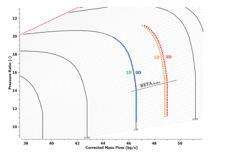
Finally, transition from the unchoked to the choked region and operation in the choked region was simulated at compressor component level only using the HPC 0D/1D component of the engine model. This was accomplished by simply specifying (at ISA conditions) a value for corrected speed NcRdes and a range of BETA values (a total of 55 values) starting from a value in the unchoked region (BETA = 0.6) to a value in the choked region (BETA = 0.05). The component was operated in both 0D and 1D mode for two values of NcRdes; one which is present in the map data (95%) and one that is between existing values (96.3%). At these NcRdes values, BETA
choke = 0.25. The setup of the simulation case was identical for both modes, meaning that choking was handled automatically in 1D mode as in 0D mode.
Figure 17 shows the operating points on the map for each of the four cases (0D and 1D modes for the two NcRdes values). For the NcRdes value present in the map data (95%), the results of both 0D and 1D modes overlap on the map speed line and demonstrate that the 1D mode is capable to transition from the unchoked to the choked region and work in the choked region. This is also shown for the other NcRdes value (96.3%), although map interpolation causes visible differences between the two modes, thus highlighting one of the 0D approach limitations.
6. Conclusions
A method for modelling multistage compressor performance using a mean-line approach, covering the entire operating region that includes choked operation has been presented. The method was materialized through the development of a dedicated component in a computational environment used for gas turbine engine modelling. The approach followed allows the integration of the mean-line model at engine level, without changing the mathematical model boundary and algebraic variables of conventional 0D map architecture.
To deal with convergence problems, posed by the simplistic nature of the mean-line equations when the compressor works near or beyond choking conditions, a formulation was developed and implemented to model choking at blade row and compressor level. Furthermore, the capability was added to allow the component developed to work in both 1D and 0D modes, even within the same simulation case. The 1D component is capable of working in both the unchoked and choked regions, without any changes to the mathematical model, while the transition from one region to the other is transparent to the user. In addition, the calculation of the choke point for the current compressor operating conditions allowed a correction to be made during 1D model execution so that the influence of any secondary effects can be taken into account. The option to perform calculations at cascade level with constant was added using only one variable (the compressor average pressure ratio) to specify an average cascade temperature for which is calculated (instead only of the inlet temperature).
Choking modelling of this level was shown, for the first time in the open literature, for the case of a multi-stage compressor for which a performance map was generated in the whole operating range. As shown, choking is calculated in a transparent way, allowing the user to know any-time where along the flow path choking has occurred and what conditions caused it.
Finally, the integration capabilities of the developed component were verified through steady state and transient simulations of a turbofan model at both altitude and SLS conditions where the new component was used as the engine’s HPC in both 0D and 1D mode. Operation in the choked region and the transition from one region to the other was demonstrated at component level. In terms of simulation times, the execution of the 1D mode with constant and halved execution time without affecting the accuracy of the results compared to the 1D mode with variable gas properties.


