A New Loss Generation Body Force Model for Fan/Compressor Blade Rows: An Artificial-Neural-Network Based Methodology

Abstract

Body force models of fans and compressors are widely employed for predicting performance due to the reduction in computational cost associated with their use, particularly in nonuniform inflows. Such models are generally divided into a portion responsible for flow turning and another for loss generation. Recently, accurate, uncalibrated turning force models have been developed, but accurate loss generation models have typically required calibration against higher fidelity computations (especially when flow separation occurs). In this paper, a blade profile loss model is introduced which requires the trailing edge boundary layer momentum thicknesses. To estimate the momentum thickness for a given blade section, an artificial neural network is trained using over 400,000 combinations of blade section shape and flow conditions. A blade-to-blade flow field solver is used to generate the training data. The model obtained depends only on blade geometry information and the local flow conditions, making its implementation in a typical computational fluid dynamics framework straightforward. We show good agreement in the prediction of profile loss for 2D cascades both on and off design in the defined ranges for the neural network training.

1. Introduction

Future turbofan engines are likely to encounter nonuniform inflows due to boundary layer ingestion (BLI) [1] or reduced length nacelles [2]. Nonuniform inflow simulations of fan/compressors require very significant computational resources if these simulations include the detailed geometry of the blades [3,4], since the computations must be time-accurate. The computational cost of nonuniform inflows in fans becomes prohibitive when multiple configurations must be considered in the design process.

The body force approach in fan/compressor simulations has been a remedy to decrease cost while maintaining accuracy in blade response to nonuniform inflow [5,6]. The body forces, implemented as source terms in the governing equations in the rotor/stator swept volumes, cause the flow turning and losses. The body force model in computational fluid dynamics (CFD) was implemented for compressors for the first time by Gong et al. [7] in 1999. That model uses bladed Reynolds-averaged Navier-Stokes (RANS) simulations or experimental data to calibrate the flow turning and viscous forces. Calibrated body force models have also shown good accuracy in analysing the aeroacoustic response of fans to nonuniform inflow [8], and they can capture dynamic instabilities in compressors [9].

There have been improvements in viscous body force models. Xu [10] in 2003 implemented a drag coefficient based loss model. That model requires bladed RANS simulations to obtain the drag coefficient for calibration, and its disadvantage is that in the case of flow separation on the blade, the drag coefficient does not represent the entire generation of entropy. Peters et al. [2] in 2015 showed an improvement of Gong’s loss model, which uses the local relative Mach number and calibration coefficients from the peak-efficiency condition. The model performs better in stall and choke conditions compared to Gong’s model. Hill and Defoe [11] used Peters’ viscous model, adding off-peak efficiency for calibration parameters to capture choke condition losses in the transonic regime.

Research on loss body force models has turned to uncalibrated approaches to make the simulations independent of bladed RANS computations, reducing the computational cost. Hall et al. in 2017 [12] introduced an inviscid loading model that accurately captures the flow turning in subsonic and transonic compressors. In terms of loss models, there has also been some progress. Guo and Hu in 2017 [13] presented a simplified analytical loss coefficient which yields the entropy generation along the streamline. That loss model is an empirical correlation and is derived for National Advisory Committee for Aeronautics (NACA) blades. Righi et al. [14] in 2018 used empirical data-driven loss models in body force simulations to capture stall/surge dynamics. However, the simulations are limited to a specified range of operating conditions. New developments in parallel force models have been implemented for nonuniform inflows in fans by using a simple empirical-based correlated model for turbulent flow over a flat plate [15,16]. The model used in the two latter references does not include the momentum thickness Reynolds number which is relevant when the flow is separated on the blade. Benichou et al. [16] showed that the loss coefficient from the body force model has a discrepancy with the bladed unsteady Reynolds-Averaged Navier–Stokes (URANS) simulations in the stator for a nonuniform inflow.

Recent studies show that the research gap in the field of loss modelling is to have a general model by considering the solution of the boundary layer equations accounting for flow separation effects.

One way to have an accurate entropy generation prediction in turbomachinery has been proposed by Denton [17]. That model requires the local boundary layer dissipation coefficient along the relative streamlines. In order to predict the dissipation coefficient applied to separated-flow conditions, it is possible to employ the two-equation boundary layer model presented by Schlichting in [18]. That two-equation boundary layer model requires closure terms. Drela and Giles [19] introduced reliable closure terms for both the laminar and turbulent regimes. Using Denton’s entropy generation approach and Drela’s boundary layer equations, Pazireh and Defoe [20] introduced a body force model in which the boundary layer equations are implemented using transport equations, convecting momentum thickness, shape factor parameter, shear stress coefficient, and the amplification ratio along the relative frame streamlines. That model has two drawbacks. First, it requires a loading model that provides the velocity distribution on either side of the blade. Hall’s loading model [12] only turns the flow towards the camberline (minimizing the local deviation), but it does not predict the velocity distribution. In 3D compressors, there is still no loading model to precisely come up with the suction and pressure-side velocity distributions. Second, the model used by Pazireh and Defoe involved one-way coupling so that the viscous model does not include the effect of the boundary displacement thickness on the velocity. In the case of flow separation, that model needs to force the shape factor parameter to have a limited gradient to avoid Goldstein’s singularity problem.

Based on the previous loss models, it seems that a reliable viscous-inviscid interaction model is required to capture the flow separation effects on the entropy generation. Youngren [21] has introduced the calculation of relative total pressure drop from the leading to trailing edge using boundary layer and flow quantities at the trailing edge.

In this paper, a new loss model based on Youngren’s approach is introduced in the form of a volumetric force for body force simulations. The model only requires the boundary layer momentum thickness at the trailing edge; a series of assumptions are made to enable estimation of trailing edge velocity and Mach number at any local cell within the blade row swept volume. Due to the body force limitations related to obtaining velocity distributions on either side of the blade and also due to high computational costs for the solution of Drela’s boundary layer equations, a data-driven approach has been used in this study to provide a direct analytical model to predict the trailing edge normalized momentum thickness. Neural networks have shown robust performance in turbomachinery applications in previous studies [22,23]. For the present paper, an automated CFD data generation Python code was combined with the 2D cascade code MISES [24] to generate over 400,000 blade-to-blade flow fields. The dataset was given to a neural network to be trained and to provide an analytical equation for calculating normalized momentum thicknesses on either side of the blade. The equation is used in the new viscous body force model.

The key findings are: (1) the new viscous body force model captures the viscous-inviscid interaction effects on the relative total pressure drop, (2) a novel momentum thickness equation shows that the machine-learning-based approach is a reliable, fast model that predicts the loss both on and off-design.

This paper introduces the new viscous loss model for 2D cascades. In addition, a new shock loss body force model based on Denton’s shock entropy generation equation [17] is introduced. The validity of the models are discussed. Implementation of the new viscous and shock loss models on a 3D compressor for uniform and nonuniform inflows is discussed in Pazireh’s PhD dissertation [25].

2. Governing Equations

Since the effect of the loss physics is taken into account with the parallel body force, the Euler equations are sufficient to employ in CFD computations, with lower costs compared to RANS solvers. The Euler equations used with the body force model are:

$$\nabla ·\left(\rho \overrightarrow{V}\right)=0$$

(1)

$$\rho \overrightarrow{V}·\nabla \left(\overrightarrow{V}\right)+\nabla p=\overrightarrow{f_n}+\overrightarrow{f_p}$$

(2)

$$\rho \overrightarrow{V}·\nabla \left(h_t\right)=\rho r\Omega f_{\theta }$$

(3)

$$\nabla \left(\rho \overrightarrow{V}\varphi \right)=0$$

(4)

where $\varphi$ is any scalar for additional transport equations for the leading edge relative Mach number, incidence angle, and Reynolds number to have these parameters in all cells within the body force swept volumes. $\overrightarrow{f_n}$ and $\overrightarrow{f_p}$ are the source terms accounting for normal and loss (viscous/shock) parallel forces, respectively, with the unit of force per volume (in SI $\frac{N}{m^3}$). $h_t$ is the specific total enthalpy, $\Omega$ is the blade row rotational speed, $\overrightarrow{V}$ is the velocity vector in the absolute frame, and $\overrightarrow{W}$ is the velocity vector in the relative frame. $f_{\theta }$ is the circumferential component of the body forces. The first term on the right hand side of Equation (3) refers to the work input by the rotor rotation and circumferential force and the second term corresponds to work done by viscous forces.

$\overrightarrow{f_p}$ acts in the opposite direction of the relative streamline and its magnitude is calculated using Equation (19). The flow turning force vector ($\overrightarrow{f_n}$) is normal to the relative streamline and is computed using Hall’s model [12]:

$$f_n=\frac{\left(2\pi d\right)\left(0.5\rho W^2\right)}{|n_{\theta }|\left(\frac{2\pi r}{B}\right)}$$

(5)

where d is the local relative streamline deviation angle from the blade camber surface.

3. Blade Viscous Loss Force Modelling Approach

Youngren’s loss model predicting the relative total pressure drop along the streamline from the leading to trailing edge is [24]:

$${\overline{\Delta p}}_{t,loss}^M=p_{t,inlet}-p_{t,exit}={\left[\frac{p_{te}}{p_e}\frac{{\rho }_e^2{W}_e^3}{\dot{m}}b\theta \right]}_{TE}$$

(6)

where b is the streamtube width, $\Delta {\overline{p}}_{t,local}^M$ is the mass-averaged total pressure loss, $\theta$ is the boundary layer momentum thickness, $\dot{m}$ is the mass flow rate, $W_e$ is the boundary layer edge velocity, ${\rho }_e$ is the boundary layer edge fluid density and $p_{te}$ and $p_e$ are the edge total pressure and static pressure, respectively.

To have a volumetric viscous force, a series of assumptions are made:

• The flow velocities and densities on either side of the trailing edge are equal and uniform outside of the boundary layer.
• The deviation at the trailing edge is negligible ($cos\left({\beta }_{TE}\right)\approx cos\left({\kappa }_{TE}\right)$).
• Boundary layer blockage caused by the displacement thickness may be neglected. This assumption is valid for attached flows. In the fully attached boundary layers, the displacement to pitch ratio is less than 5% [25]. Since an artificial neural network (ANN) is used to assess the momentum thickness on either side of the airfoil at the trailing edge, adding the displacement thickness to the outputs reduces the accuracy of the data-driven approach. Thus, the displacement thickness is skipped for simplification purposes.
• The flow is assumed to be isentropic outside of the boundary layer. The shock losses are modelled separately. This implies that:

  $$\frac{p_{te}}{p_e}={(1+0.2M_{rel}^2)}^{\frac{\gamma }{\gamma -1}}$$

  (7)

  where $M_{rel}$ is the relative Mach number.
• The contraction in passage area has a low impact on the flow velocity and the radial velocity is negligible.

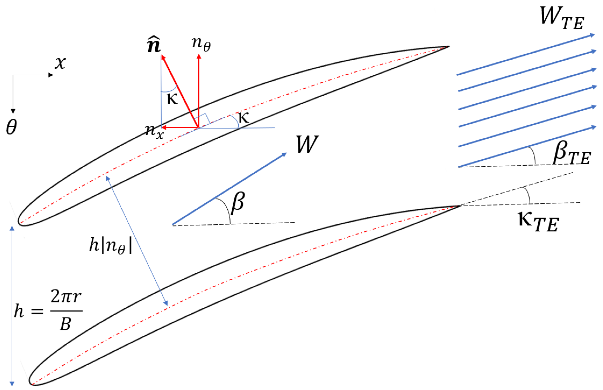
A schematic of a 2D cascade illustrating the relative flow and blade metal angles, as well as the unit normal to the camber line and its components, is depicted in Figure 1. It can be seen that, in a 2D cascade, the circumferential component of the camber unit normal is equivalent to the cosine of the blade metal angle. We adopt the normal-based notation as it generalises to 3D blade rows without modification. Applying the assumptions about the flow uniformity and direction at the trailing edge allows the mass flow through the passage to be written in terms of trailing edge quantities:

$$\dot{m}={\rho }_{TE}{W}_{TE}{\left|n_{\theta }\right|}_{TE}\left(h-{\delta }_{TE}^{*}\right)b$$

(8)

where h is the pitch.

In most blade rows, area contractions are used to maintain constant axial velocity at design. Taking into account mass continuity under steady-state conditions, any local axial velocity can be directly related to the trailing edge velocity:

$$W_{TE}=\frac{W_x}{|n_{\theta }{|}_{TE}}$$

(9)

Although Equation (9) originates from several strong assumptions, it is a sensible approach to relate the trailing edge velocity to the local axial velocity. A detailed discussion about the valid and invalid regions of these assumptions in a 3D compressor can be found in [25]. The flow between 20% and 80% span generally satisfies the assumptions. In 2D cascades, which are the focus of this paper, the accuracy is over 90% for different compressor airfoils.

Similarly, considering constant sound speeds in the row (as it occurs in compressors), the axial Mach number is related to the trailing relative Mach number:

$$M_{rel,TE}=\frac{M_x}{|n_{\theta }{|}_{TE}}$$

(10)

Substituting Equations (7) to (10) into Equation (6) gives an expression for the relative total pressure loss from the leading to the trailing edge in terms of the local $M_x$, $\rho$, $W_x$ and ${\theta }_{TE}$ values:

$$\Delta p_{t,rel}=f\left(M_x,\rho ,W_x,{\left|n_{\theta }\right|}_{TE},{\theta }_{TE},B,r\right)$$

(11)

where B is number of blades in the row, $n_{\theta }$ is the circumferential component of normal vector to the camber surface, c is the chord length, and $W_x$ is the local axial velocity in the body force calculations. The local loss body force is calculated as:

$$f_p=\frac{d{p}_{t,rel}}{d\xi }$$

(12)

where $\xi$ represents the relative streamline direction. We further assume that the loss is roughly distributed evenly from the leading to trailing edges, so that Equation (12) with the previous assumption that the chord and camber arc lengths are almost equal in compressor airfoils yields:

$$f_p=\frac{d{p}_{t,rel}}{d\xi }\approx \frac{\Delta p_{t,rel}}{c}$$

(13)

Thus, combining Equations (11) and (13), the volumetric loss body force is:

$$f_{p,viscous}=\frac{{(1+0.2{\left(\frac{M_x}{|n_{\theta }{|}_{TE}}\right)}^2)}^{3.5}\rho W_x^2}{\left(\frac{2\pi r}{B}\right)\left(\right|n_{\theta }{{|}_{TE})}^3}\left(\frac{{\theta }_{TE,SS}+{\theta }_{TE,PS}}{c}\right)$$

(14)

This model accounts for the loss within the blade row and does not take into account downstream mixing losses. From Equation (14) it can be seen that in 2D body force applications, the only parameter not based on known geometry or local flow is ${\theta }_{TE}$. Therefore, the aim is to have an analytical equation that calculates ${\theta }_{TE}$ without needing to add the boundary layer differential equations to the computations.

4. Blade Shock Loss Force Modelling Approach

Denton introduced an equation for the entropy rise from weak shocks in terms of the local relative Mach number [17]:

$$\Delta s\approx c_v\frac{2\gamma \left(\gamma -1\right)}{3{\left(\gamma +1\right)}^2}{\left(M_{rel}^2-1\right)}^3$$

(15)

where $c_v$ is specific heat at constant volume and $\gamma$ is the isentropic expansion factor (heat capacity ratio).

Neglecting radius change effects, the relative total pressure is related to the entropy rise using Gibbs’ equation:

$$\Delta s=-R\frac{\Delta p_{t,rel}}{p_{t,rel}}$$

(16)

where R is the specific gas constant.

Assuming that normal shock waves appears with local supersonic relative flow, Denton’s shock loss in Equation (15) can be inserted in Equation (16) to get the changes of relative total pressure:

$${\left(p_{t,rel,LE}-p_{t,rel,TE}\right)}_{shock}=p_{t,rel}\frac{c_v}{R}\frac{2\gamma \left(\gamma -1\right)}{3{\left(\gamma +1\right)}^2}{\left(M_{rel}^2-1\right)}^3$$

(17)

The shock loss prediction presented in Equation (17) is appropriate for normal shocks [17]. Thus, it overpredicts the shock loss with the same relative Mach number for oblique shocks. A volumetric shock loss model is obtained by dividing the total pressure change by the staggered blade spacing:

$$f_{p,shock}=\left\{\begin{array}{cc}\frac{p_{t,rel}\frac{c_v}{R}\frac{2\gamma \left(\gamma -1\right)}{3{\left(\gamma +1\right)}^2}{\left(M_{rel}^2-1\right)}^3}{\left(\frac{2\pi r}{B}\right)\left|n_{\theta }\right|}\hfill & M_{rel}>1\hfill \\ 0\hfill & M_{rel}\le 1\hfill \end{array}\right.$$

(18)

The total volumetric loss force is:

$$f_p=f_{p,shock}+f_{p,viscous}$$

(19)

It should be reiterated that the volumetric loss source terms are distributed along the axial direction in the blade row swept volume in body force CFD simulations where the local terms are applied to every cell within the body force zone.

5. Artificial Neural Network to Estimate Trailing Edge Momentum Thickness

The fact that there was no a priori sense of what the functional form of correlations for ${\theta }_{TE}$ should be requires the use either of traditional response surface methods or else an ANN. An ANN is just another form of response surface. We chose to use an ANN due to their prior successful use in turbomachinery applications as outlined in the introduction. A neural network was trained using over 400,000 CFD computations to provide an analytical equation predicting the momentum thickness of the boundary layer at the trailing edge of an airfoil on either side of it. The method of Xiaoqiang et al. 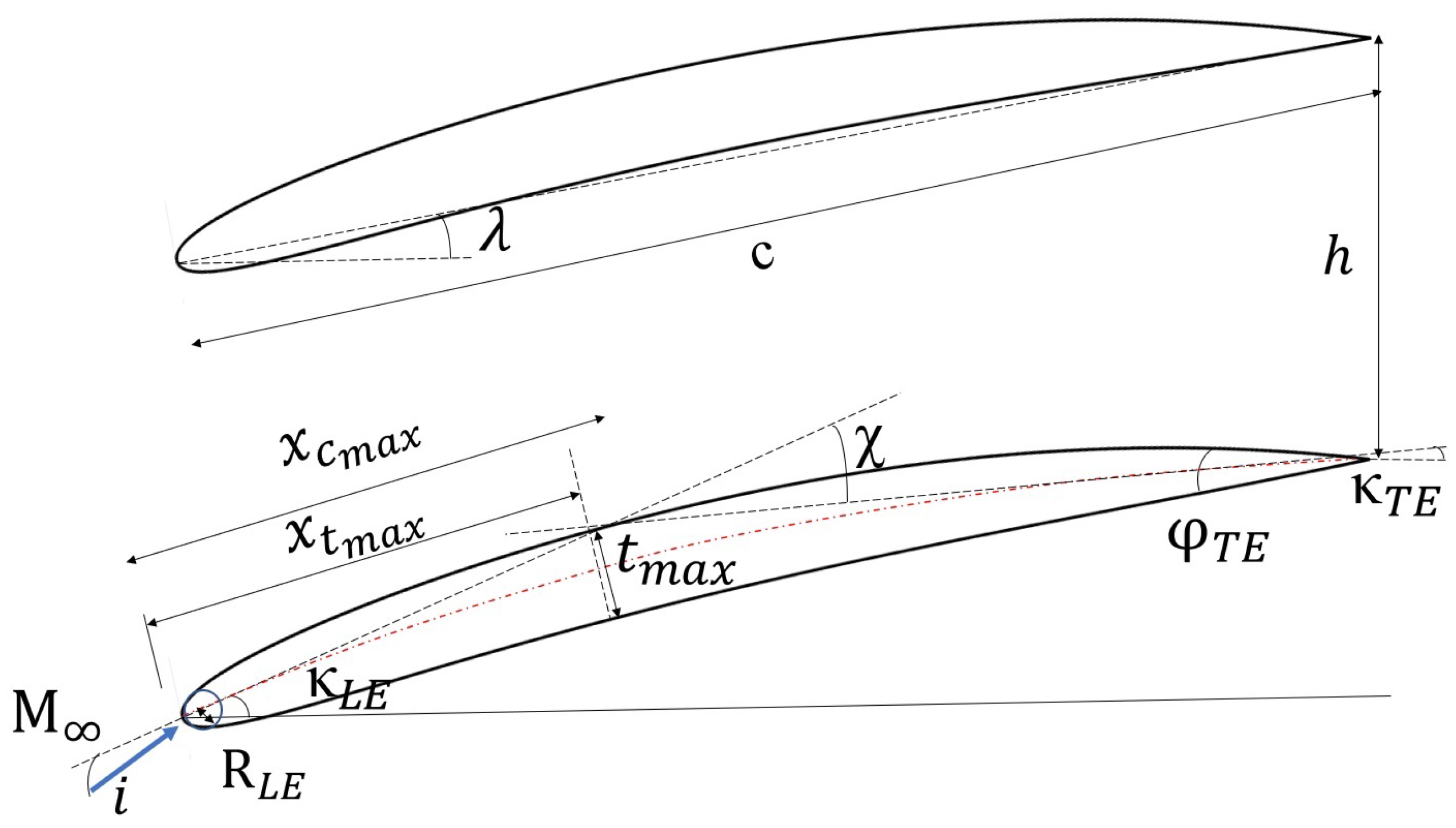[26] was used to define the camberline and thickness parametrically. A comprehensive study for the current paper showed that the flow Reynolds number, incoming relative Mach number, and incoming flow incidence angle are the effective flow properties determining the viscous conditions. Camber, thickness, position of maximum camber to chord ratio, position of maximum camber to chord ratio, boat-tail angle, and leading-edge radius to chord ratio implicitly determine the velocity distribution, which by itself, influences the viscous behaviour around the blade. Thus, the variables shown in

Table 1. Ranges for data generation from computational fluid dynamics (CFD) used in artificial neural network and steps.

Parameter	Range	Step
$\frac{t_{max}}{c}$	0.025–0.15	0.025
$\frac{x_{t_{max}}}{c}$	0.3–0.5	0.1
$\chi$(deg)	10–40	15
$\frac{x_{c_{max}}}{c}$	0.4–0.6	0.1
i (deg)	($-6$)–(6)	1
$M_{\infty }$	0.2–1.6	0.2
$R{e}_c$	$1\times {10}^5$–$1.51\times {10}^6$	$4.7\times {10}^5$
$\frac{c}{h}$	0.5–2	0.5
$\frac{R_{LE}}{c}$	0.001–0.021	0.005
${\phi }_{TE}$ (deg)	0–10	5

were used to produce MISES CFD simulations for the ANN. These parameters are the attributes influencing the trailing edge momentum thickness. c is the chord length, h is the pitch, $R_{LE}$ is the leading edge radius, $t_{max}$ is the maximum thickness, $x_{t_{max}}$ is the position of maximum thickness, $\chi$ is the airfoil camber, $x_{c_{max}}$ is the position of maximum camber, $\sigma$ is the chord to spacing ratio, ${\phi }_{TE}$ is the trailing edge boat-tail angle, and i is the incidence angle.

The boundary layer momentum thickness can be influenced by the free-stream turbulence intensity. However, this physical parameter was not considered in the simulations in order to avoid increasing the dataset features for neural network training.

Figure 2 shows the nomenclature used for the 2D cascade calculations.

In a previous study [27] it has been shown that one hidden-layer in the ANN is adequate for compressor problems. Here, a 40-node hidden-layer feed-forward back-propagation neural network has been used. There are 10 input nodes (the attributes shown in Table 1) and 2 nodes in the output layer: the trailing edge momentum thickness for either side of the blade. There are no specific criteria for the optimum architecture in a neural network. However, from one to three layers with ten to forty neurons were tested to assess the optimum structure.

Hyperbolic tangent sigmoid functions were used as transfer (activation) functions. This function is defined to be

$$tansig\left(a\right)=\frac{2}{1+e^{-2a}}-1$$

(20)

where a is any input variable. The accuracy of the ANN was assessed using the root mean square (RMS) error for all $\mathcal{N}$ samples in the dataset:

$$RMSerror=\sqrt{\frac{{\sum }_{d=1}^{\mathcal{N}}{(y_{actual,d}-y_{prediction,d})}^2}{\mathcal{N}}}$$

(21)

where $y_{actual}$ is the actual output in dataset and $y_{prediction}$ is the ANN prediction for the output. In the back-propagation algorithm, gradient optimisation is used to minimise the RMS error.

The analytical equations to predict the normalised momentum thickness (momentum to chord ratio) on either side of the blade are:

$$F_{1,i}=2\frac{\left(X_i-X_{min,i}\right)}{X_{max,i}-X_{min,i}}-1i=1,...,10$$

(22)

$$F_{2,j}=\frac{2}{1+e^{-2\left({\sum }_{i=1}^{10}{w}_{1,j,i}\times F_{1,i}+b_{1,j}\right)}}-1j=1,...,40$$

(23)

$$F_{3,k}=\frac{2}{1+e^{-2\left({\sum }_{j=1}^{40}{w}_{2,k,j}\times F_{2,j}+b_{2,k}\right)}}-1k=1,2$$

(24)

$$F_{4,k}=\frac{\left(F_{3,k}+1\right)}{2}\left(y_{max}-y_{min}\right)+y_{min}k=1,2$$

(25)

where $\overrightarrow{X}$ is the input vector:

$$\overrightarrow{X}=\left[\begin{array}{c}\frac{t_{max}}{c}\\ \frac{x_{t_{max}}}{c}\\ \chi \\ \frac{x_{c_{max}}}{c}\\ i\\ M_{\infty }\\ R{e}_c\\ \frac{c}{h}\\ \frac{R_{LE}}{c}\\ {\phi }_{TE}\end{array}\right]$$

(26)

${\overrightarrow{X}}_{min}$ is a vector with the minimum values of each input variable in the entire dataset, ${\overrightarrow{X}}_{max}$ is a vector with the maximum values of each input variable in the entire dataset, ${\overrightarrow{y}}_{min}$ is a vector with the minimum values of each output variable in the entire dataset, and ${\overrightarrow{y}}_{max}$ is a vector with the maximum values of each output variable in the entire dataset. ${\overrightarrow{b}}_1$ and ${\overrightarrow{b}}_2$ are the bias vectors and the matrices $w_1$ and $w_2$ are weighting matrices. All these vectors and matrices can be found in the Appendix A of this paper.

The suction and pressure side trailing edge momentum thickness to chord ratios are:

$$\left[\begin{array}{c}\frac{{\theta }_{SS,TE}}{c}\\ \frac{{\theta }_{PS,TE}}{c}\end{array}\right]=\left[\begin{array}{c}{F}_{4,1}\\ F_{4,2}\end{array}\right]$$

(27)

6. Numerical Implementation

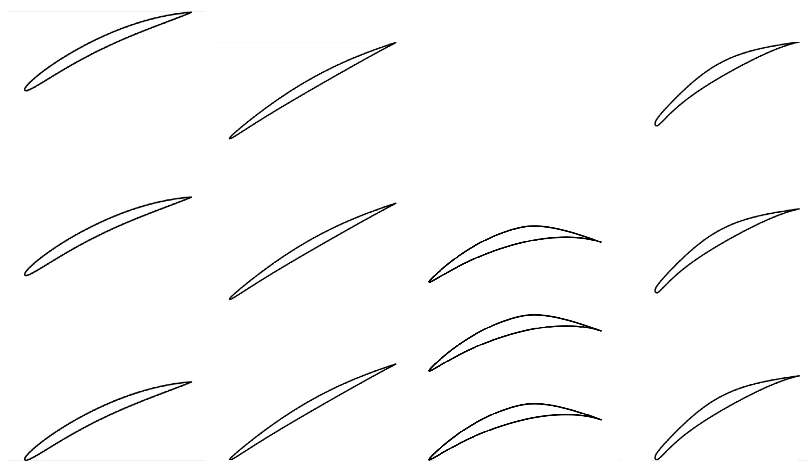
To assess the body force loss model, four cascades are considered. These cascades are shown in Figure 3. The geometry information of these cascades is shown in

Table 2. Geometry data for the cascades

Parameter	Cascade 1	Cascade 2	Cascade 3	Cascade 4
$\frac{t_{max}}{c}$	0.06	0.05	0.085	0.075
$\frac{x_{t_{max}}}{c}$	0.4	0.5	0.48	0.05
$\chi$(deg)	25	15	50	40
$\frac{x_{c_{max}}}{c}$	0.5	0.5	0.57	0.5
$\frac{R_{LE}}{c}$	0.005	0.001	0.001	0.015
${\phi }_{TE}$ (deg)	10	10	17	5
$\lambda$ (deg)	25	30	13	30
$\sigma (=\frac{c}{h})$	1.0	1.2	2.0	1.0

. Flow conditions used in the simulations for the cascades are shown in

Table 3. Flow conditions for the cascades.

Cascade	${\mathit{M}}_{\mathit{\infty }}$	Re
1	0.30	335,000
2	0.65	700,000
3	0.40	440,000
4	0.45	1,510,000

.

Each cascade is chosen to explore a particular type of compressor section or flow characteristic. Cascade 1 is a low-speed cascade with moderate camber, representative of a low-speed machine mid-span section. Cascade 2 has low camber and represents a mid-span section of a high-speed compressor, thus a higher inlet relative Mach number is used. Cascade 3 is highly cambered and represents a hub section of a fan; it also has geometric parameters outside the range of training data for the ANN so it serves as a test case for how well the model predicts loss outside that training range. Finally, cascade 4 is representative of a near-tip section of low- to moderate-speed compressor, and its geometric parameters are at the edge of the ANN training data parameter space. It is used, in conjunction with cascade 3, to compare loss predictions for highly-cambered cascades within and outside the ANN training data parameter space.

A mesh independence study was carried out to ensure the body force model is not affected by the mesh size in a 2D solver. With uniform inflow, the flow within the body force model is axisymmetric with periodic boundary conditions employed. Hall’s loading model was used for flow turning. By increasing the number of axial cells along the blade axial chord the mesh changed from coarse to fine until the loss coefficient stopped changing.

The mesh independence study was performed on cascade 1. The results are shown in

Table 4. Grid independence study for body force model in cascade 1 with $M=0.3$. Zero incidence, $\sigma =1.0$, Reynolds number based on chord $3.35\times {10}^5$.

Cells along Chord	$\mathit{\omega }$	${\mathit{\beta }}_{\mathit{TE}}-{\mathit{\beta }}_{\mathit{LE}}$ (degrees)
10	0.0126	16.8
20	0.0135	17.5
40	0.0139	17.6
60	0.0139	17.6

. Forty axial cells is sufficient. All remaining results shown in this paper are for 40 axial cells.

7. Results

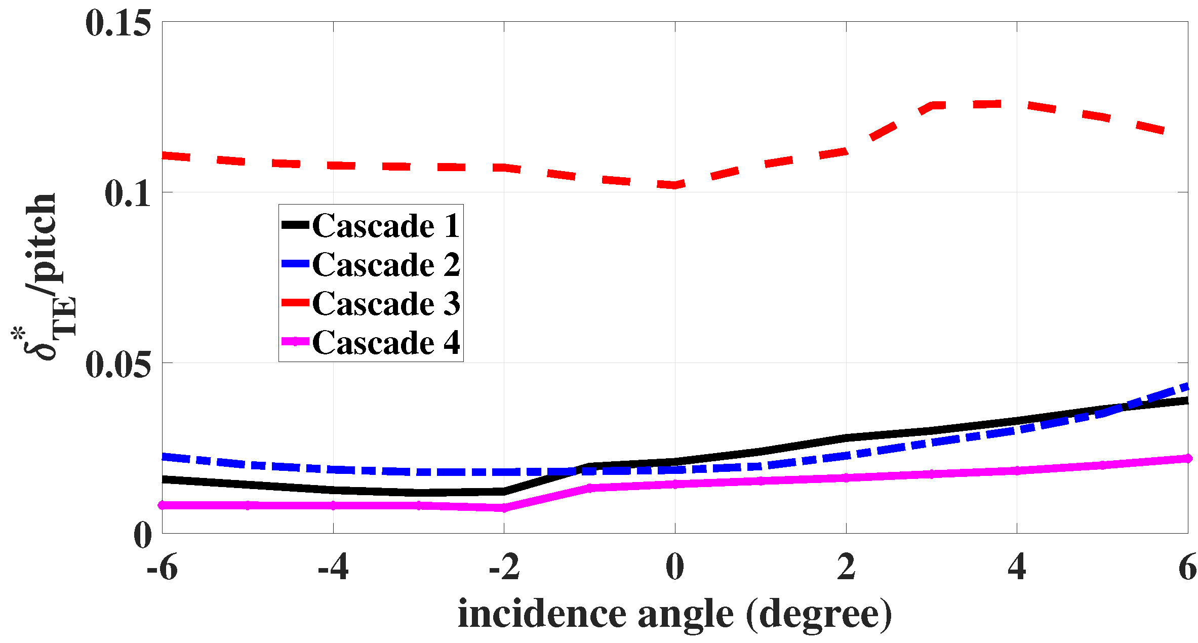
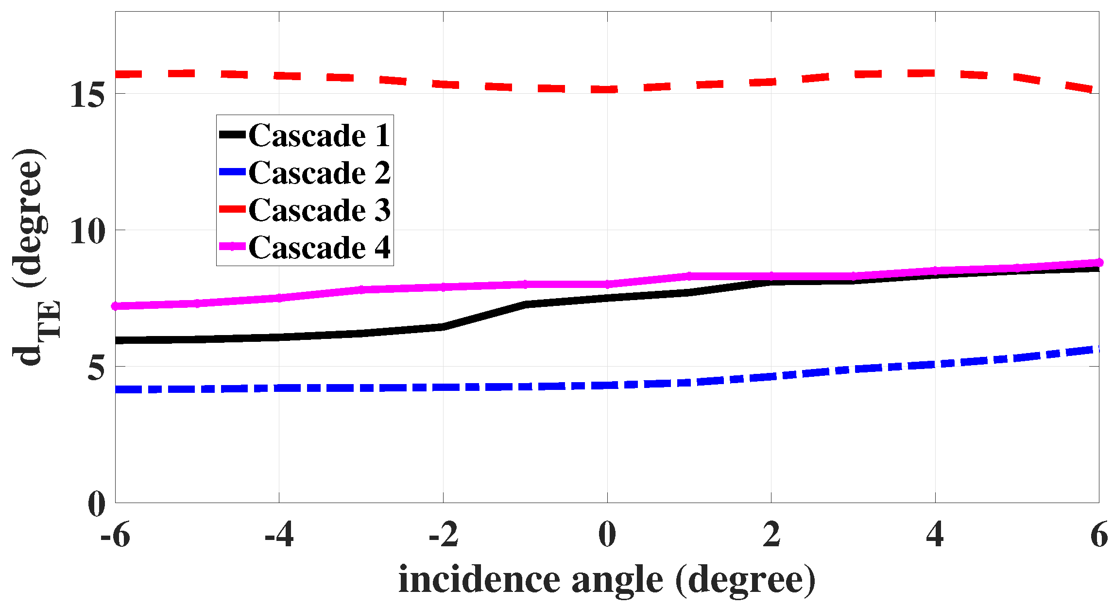
To gain further insight into the flow in the three cascades, the deviation angle and boundary layer displacement thickness at the trailing edge are evaluated from the bladed CFD simulations. The displacement thickness to pitch ratios ($\frac{{\delta }_{TE}^{*}}{pitch}$) and deviation angles ($d_{TE}={\beta }_{TE}-{\kappa }_{TE}$) for a range of −6 to 6 incidence angles for the four cascades are shown in Figure 4 and Figure 5. Cascade 1 experiences deviation angles between 6 to 9 degrees for a range of −6 to 6 incidence angles, and the maximum boundary layer displacement thickness to pitch ratio occurs at an incidence angle of 6 degrees that is 0.04. Cascade 2 encounters lower deviation so that a maximum deviation angle of 5.6 degrees occurs. Again the displacement to pitch ratio is less than 5%. However, a thick boundary layer appears for cascade 3, where the displacement thickness to pitch ratio is over 10% and the deviation angle is over 15 degrees. In cascade 3, high incidence leads to a delayed transition on the pressure side of the blade and consequently a lower boundary layer displacement thickness. Accordingly, a decrease in the boundary layer displacement thickness appears for incidence angles over 4 degrees. Higher inlet turbulence might lead to a different behaviour. The behaviour is very different than that of cascade 4, which has a maximum deviation angle of 9 degrees at the trailing edge and its displacement thickness to pitch ratio at a high incidence angle of 6 degrees is below 0.05. As a result, cascades 1, 2, and 4 are fully compatible with the viscous loss model assumptions listed earlier.

Table 5. Bladed CFD results of four cascades.

Cascade	max ${\mathit{d}}_{\mathbf{TE}}$ (degree)	max $\frac{{\mathit{\delta }}_{\mathbf{TE}}^{*}}{\mathbf{pitch}}$
1	8.6	0.039
2	5.6	0.043
3	15.7	0.126
4	8.8	0.022

summarises the maximum deviation angle and the maximum boundary layer displacement to pitch ratio at the trailing edge for all four cascades.

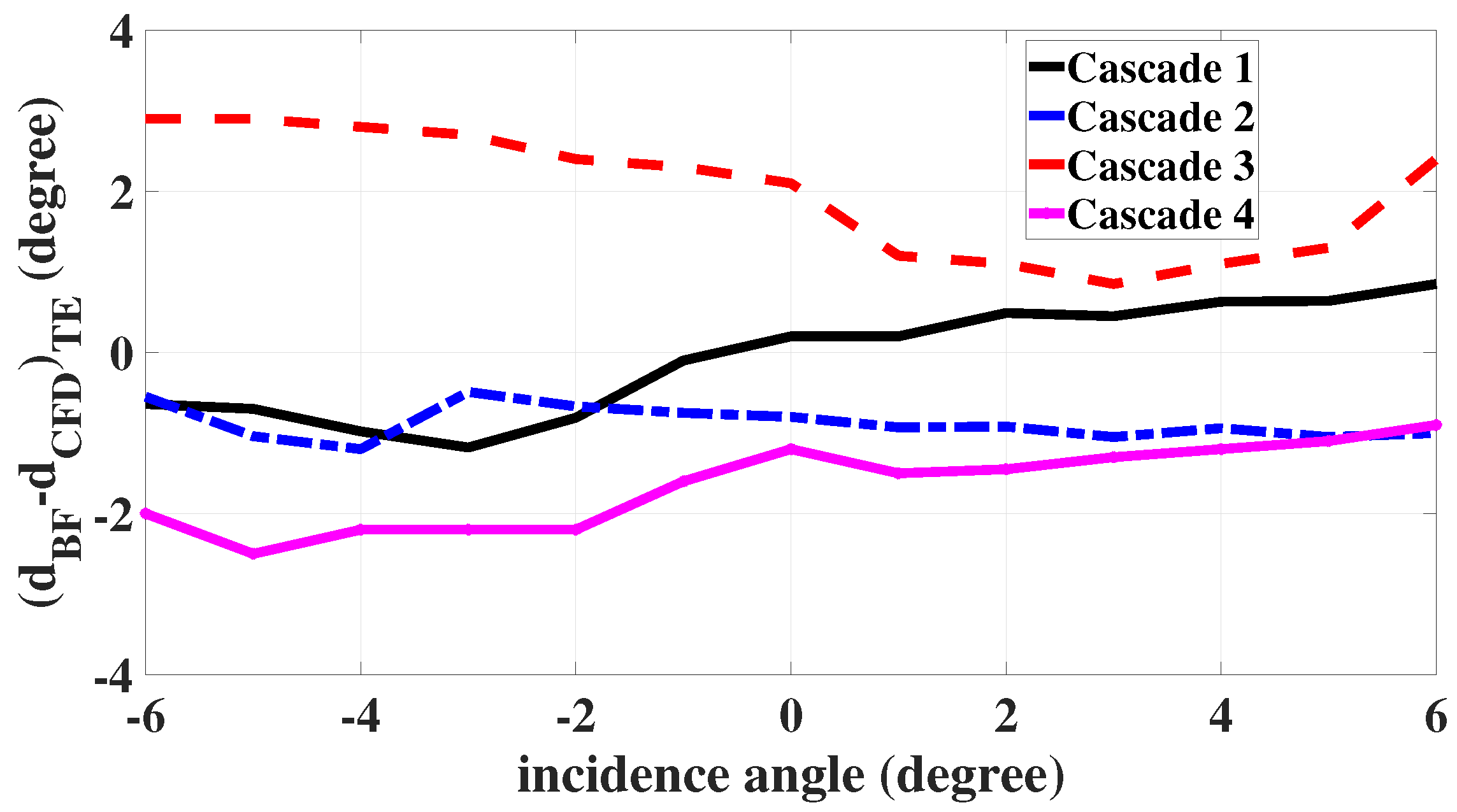
To assess the performance of Hall’s loading model for producing flow turning, the deviation at the trailing edge in the body force computations has been calculated and compared with the bladed CFD simulations. This is shown in Figure 6. While there are minor variations across the cascades and with varying incidence, in general the trailing edge deviation is well-captured by Hall’s turning force model. For the very highly cambered cascade 3, Hall’s model underpredicts the deviation; for the other cascades, it generally overpredicts it or has an error of only ∼1 degree. Two physical reasons cause the underprediction of deviation (overprediction of flow turning) for cascade 3. First, this highly-cambered cascade experiences a thick boundary layer with high displacement thickness. Hall’s turning body force model does not account for the effective airfoil thickness changing. Second, a high deviation at the trailing edge region for cascade 3 occurs in the bladed computations. While Hall’s model tends to turn the flow towards the camber surface, a high deviation and recambering are not captured by Hall’s model and it turns the flow to the initial camber angle at the trailing edge region, leading to a higher flow turning compared to the real physics. This matches with the higher total pressure increase compared to the bladed RANS simulation in the hub region of a 3D compressor rotor where a high cambered section exists [25]. Additionally, cascade 3 has a higher solidity than the other three cascades, and Hall’s model scales the turning force with solidity, leading to lower deviation. Overall, the turning model adequately predicts the deviation for the purpose of the loss model.

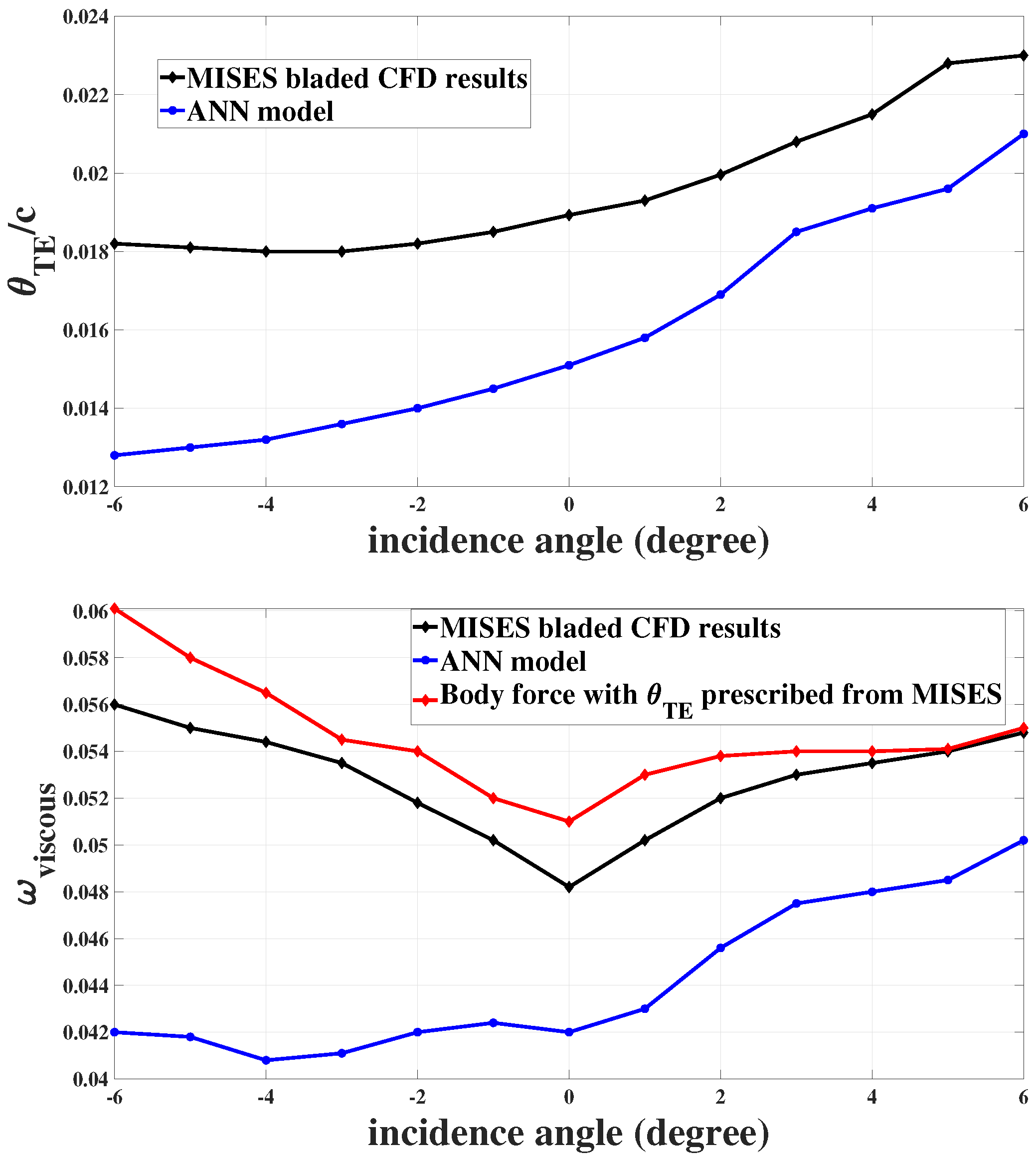
Momentum thickness ${\theta }_{TE}$ and viscous loss coefficient,

$${\omega }_{viscous}=\frac{p_{t,LE}-p_{t,TE}}{p_{t,LE}-p_{LE}}$$

(28)

for the four cascades are shown in Figure 7, Figure 8, Figure 9 and Figure 10. Cascades 1 and 2 are not part of the ANN training data, but their geometries and flow conditions are within the ranges of the training dataset. Cascade 3 has camber and a boat-tail angle which exceed the range of the training dataset. Cascade 4 is part of the training dataset.

To validate the viscous loss body force model (Equation (14)), the trailing edge momentum thicknesses from the bladed CFD simulations (MISES) are prescribed in body force computations. The results are compared with the momentum thickness from the ANN model and the MISES data in the bottom part of each of Figure 7, Figure 8, Figure 9 and Figure 10.

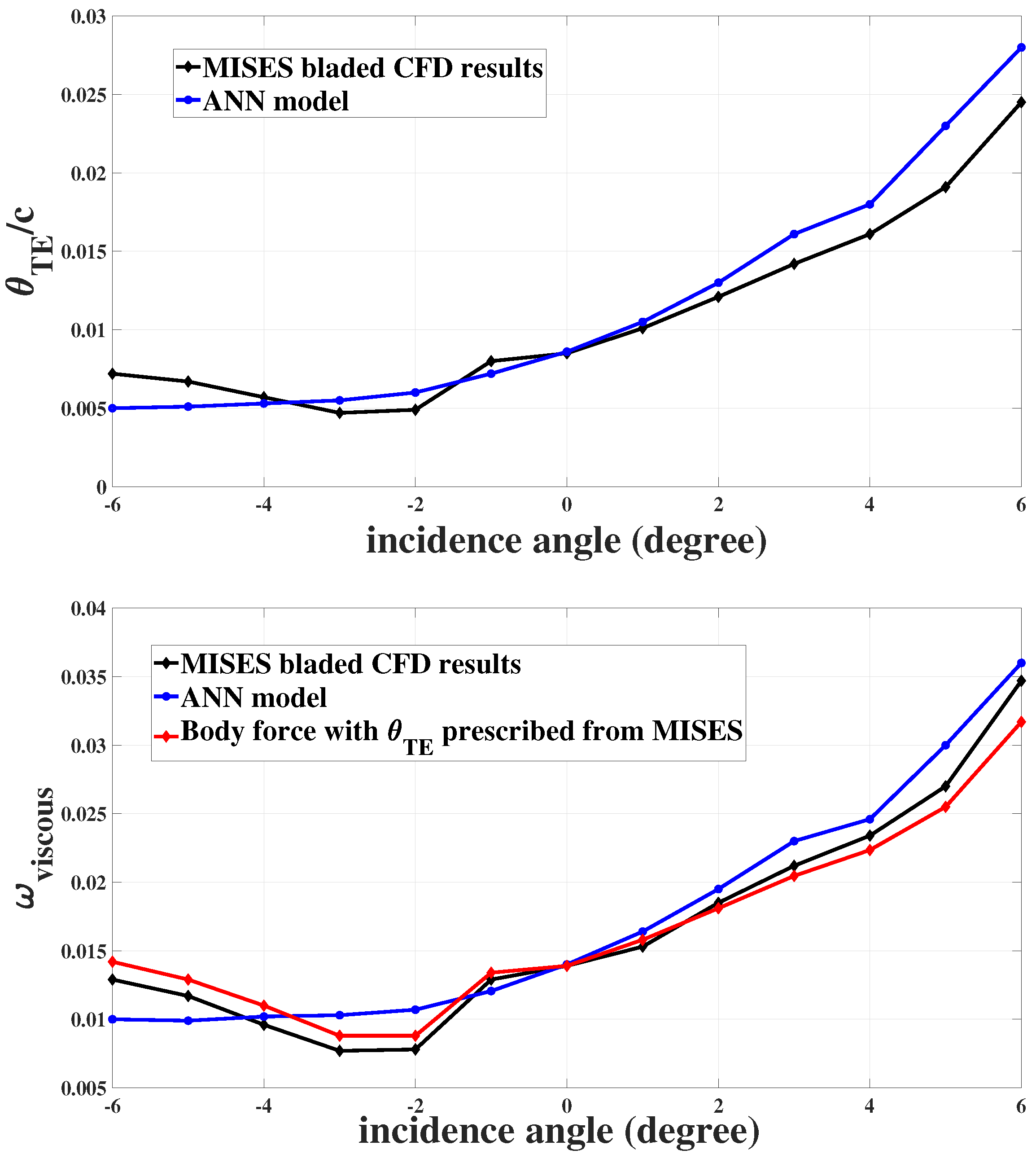
Figure 7 shows the comparison of the ANN predicted momentum thickness and loss coefficients with data from MISES for incidence angles between −6 and 6 degrees for cascade 1. The maximum error in predicted momentum thickness (upper part of figure) is at an incidence angle of −6 degrees, where the error is $26\%$. Overall the trend is well-captured, though accuracy decreases in general as one moves away from zero incidence. With regards to loss (lower part of figure), which is the ultimate aim of the viscous body force, prescribing ${\theta }_{TE}$ yields an accurate prediction at all incidence angles (maximum error of $7\%$), while the ANN performs well except at strong negative incidence, where it fails to capture the rise in loss. Referring back to the upper part of the figure, it can be seen that this trend stems from the ANN prediction of momentum thickness.

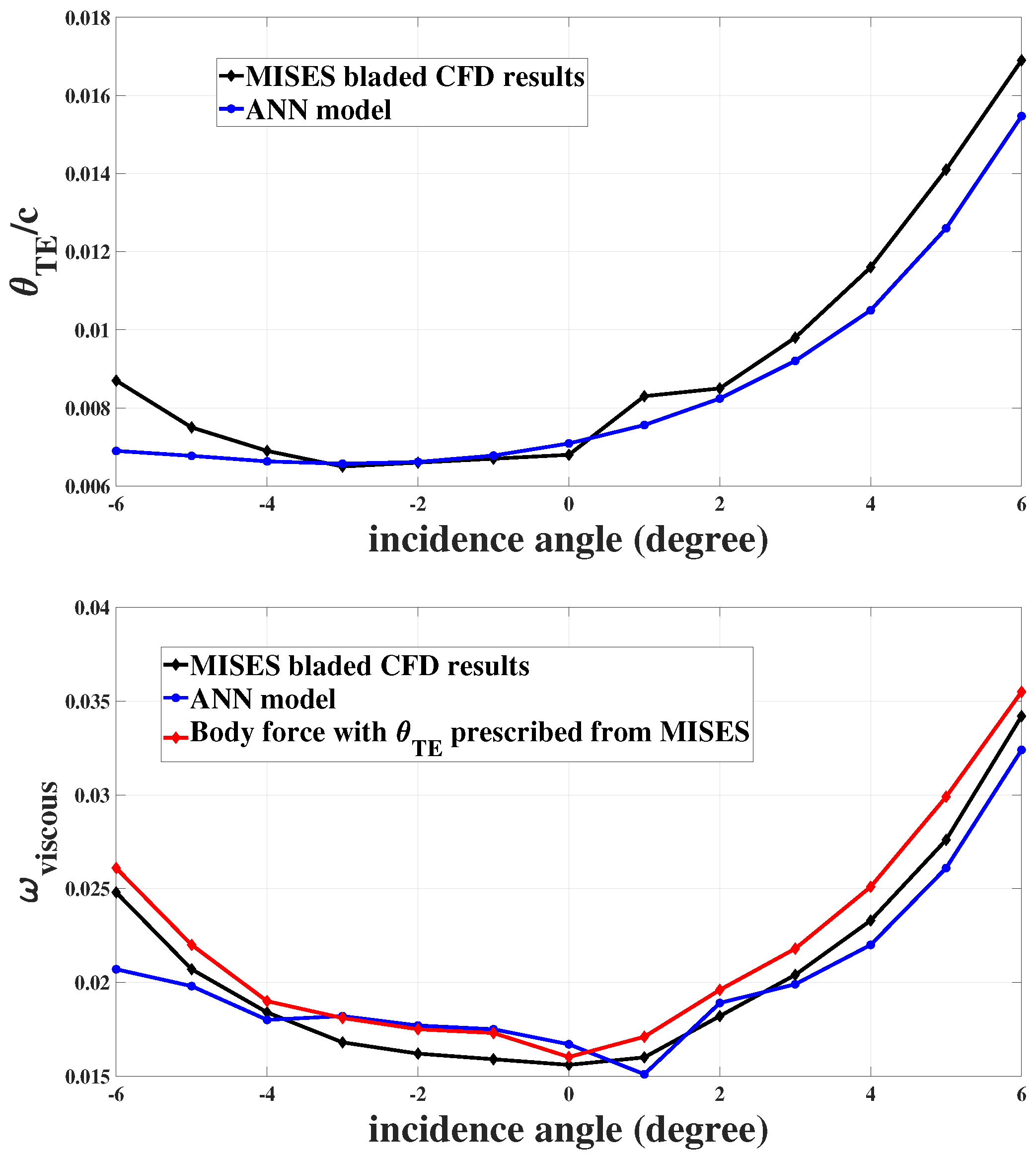
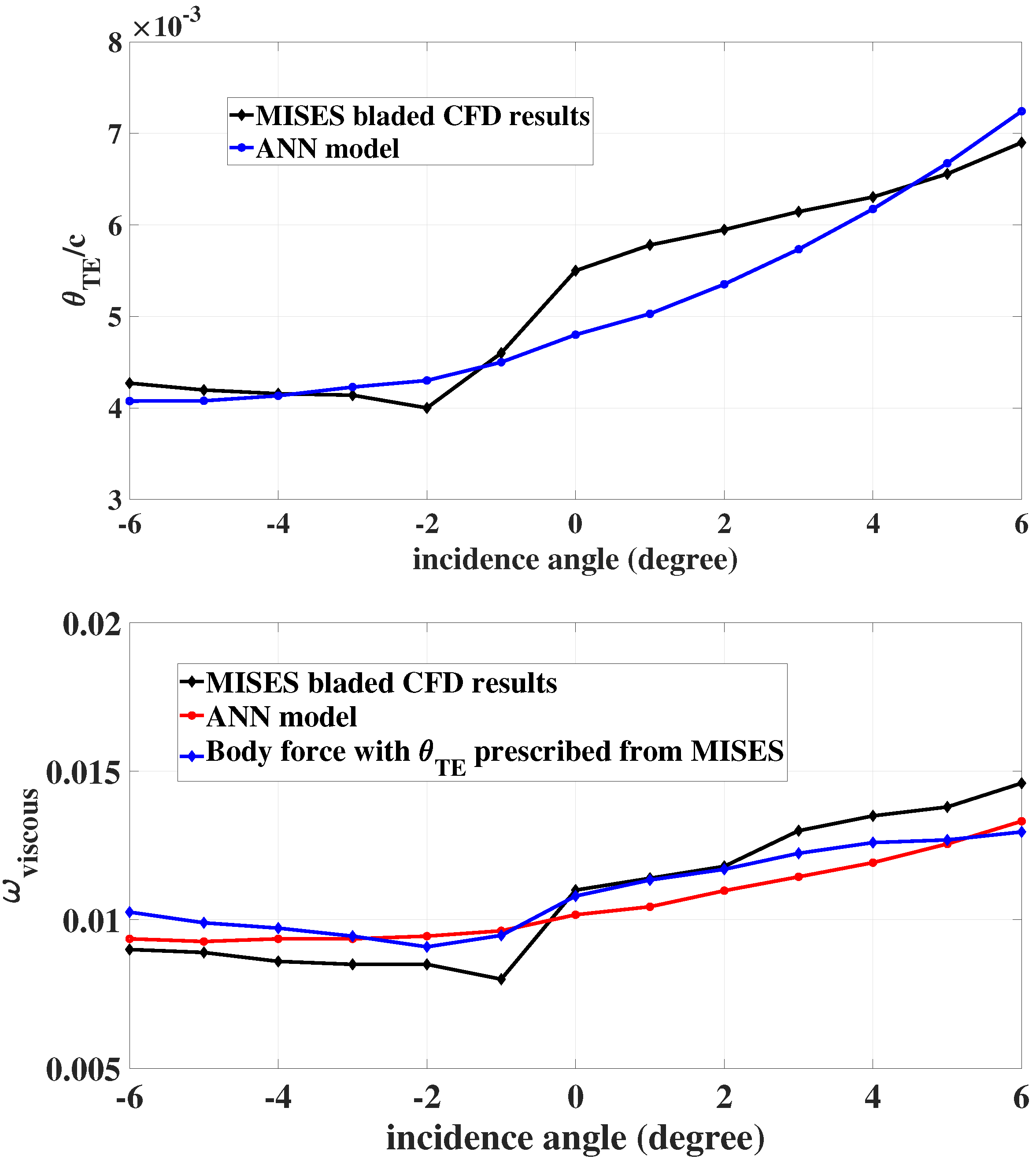
Figure 8 shows the same comparison for cascade 2, for which the flow is subsonic but compressible ($M_{\infty }=0.65$). The ANN model underpredicts the momentum thickness for incidence smaller than $-3$ degrees and larger than $+2$ degrees. The trend at high incidence is well-captured but the ANN again fails to capture the trend of rising momentum thickness at the most negative incidence values considered. In the lower part of Figure 8, the impact of this underprediction of momentum thickness manifests in the loss in a similar way as for cascade 1. Here, however, the compressible nature of the flow contributes to the fact that the trend, at least, is captured at negative incidence. Here the axial Mach number drops from 0.52 to 0.45 from the leading to trailing edge. Since in Equation (14) the local force scales with $\rho W_x^2$ but the loss model is formulated based on trailing edge quantities, the decreasing axial velocity associated with this Mach number change more than offsets the density rise, and the loss force distribution becomes fore-loaded, increasing loss for incidence less than $-4$ degrees despite the failure of the ANN to predict the increasing momentum thickness.

Recall that as a highly cambered airfoil, cascade 3 is modelled to assess the impact of large deviation. Figure 9 shows the same type of data as for the first two cascades but for cascade 3. Clearly, the ANN is unable to predict ${\theta }_{TE}$ qualitatively or quantitatively for this cascade. This has a dramatic impact on the loss prediction as can be seen in the lower part of the figure. Since Equation (14) contains a term with the cube of the cosine of the blade metal angle at the trailing edge, which is a surrogate for the trailing edge relative flow angle under the assumption that the trailing edge deviation angle is small. For cascade 3, a deviation of approximately 15 degrees occurs, as was shown in Figure 5. The cube of the cosine of that 15-degree difference in the calculations can create an error of over $10\%$ in loss coefficient, which compounds the error in predicted ${\theta }_{TE}$ coming from the ANN.

To assess whether high camber alone is responsible for the poor ANN predictions, we examine cascade 4, which has 40 degrees of camber but is within the training dataset for the ANN. As the trailing edge momentum thickness results show in the upper part of Figure 10, the model captures the trailing edge momentum thickness variations correctly and the worst predictions have a maximum error of 12% at low incidence angles where the airfoil is sensitive to incidence variations due to a blunt leading edge. When prescribing the momentum thickness from the bladed simulations, a maximum error of 13% for the loss coefficient at a high incidence angle of 6 degrees is predicted. As camber increases, the assumption that the length of a relative streamline through the blade row is equal to the chord becomes less accurate, leading to loss underprediction. However, clearly the predictions are much better here than for cascade 3 and it appears that so long as the cascade geometry and flow conditions are within the range of the dataset training parameters, the ANN and loss model will produce reasonably accurate predictions.

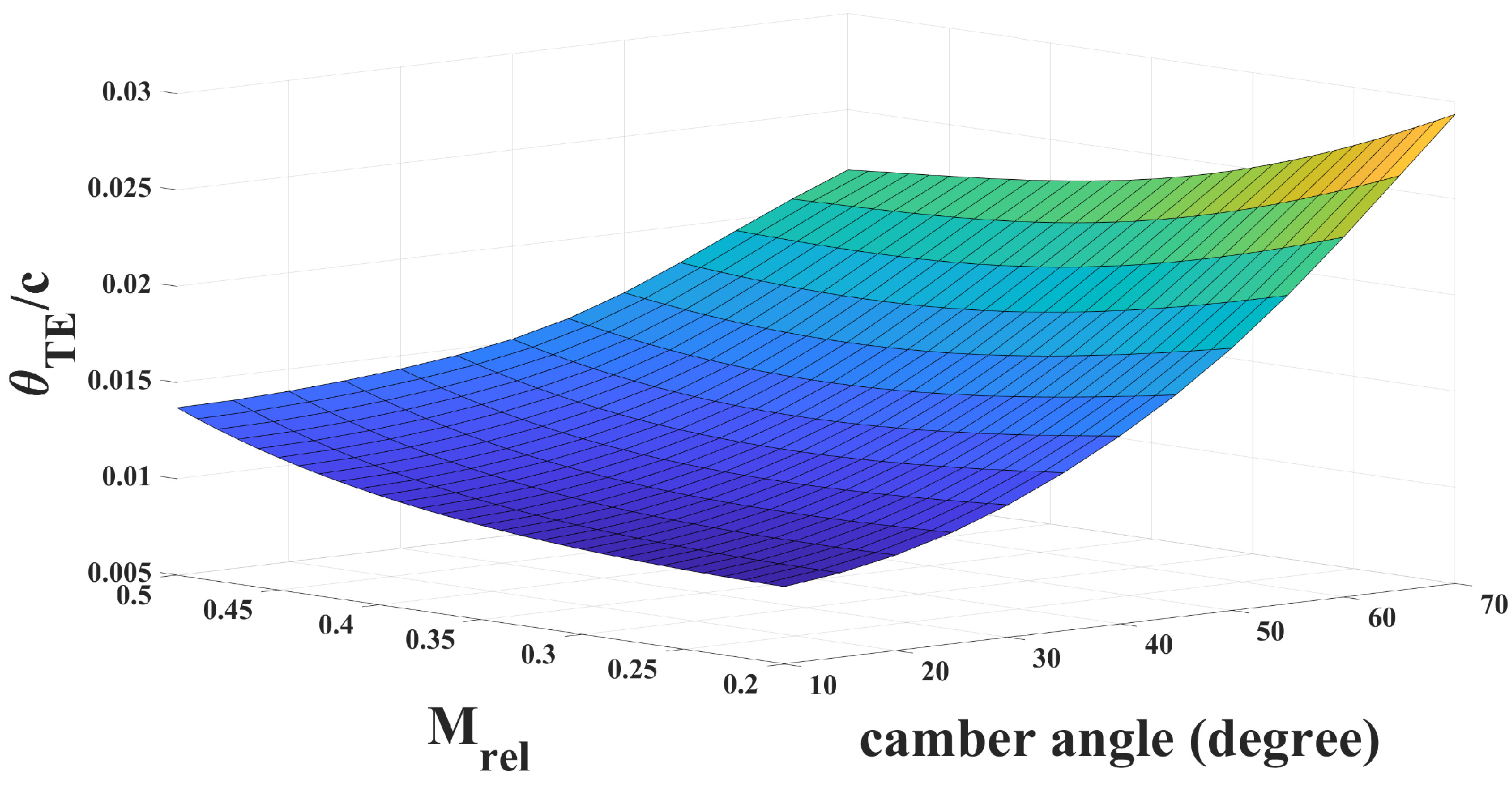
To show how the ANN model performs beyond the defined range for the camber angles, Figure 11 illustrates the normalised trailing edge momentum thickness for a range of Mach number and the range of camber angles from 10 to 70 degrees, with all other parameters corresponding to those for cascade 1. It can be seen that the model predicts an increasing trend of the momentum thickness for high camber angles even though the training data did not include those incidence angles. This implies that the model will roughly capture trends for high camber cases, though quantitative results will be inaccurate as was shown for cascade 3.

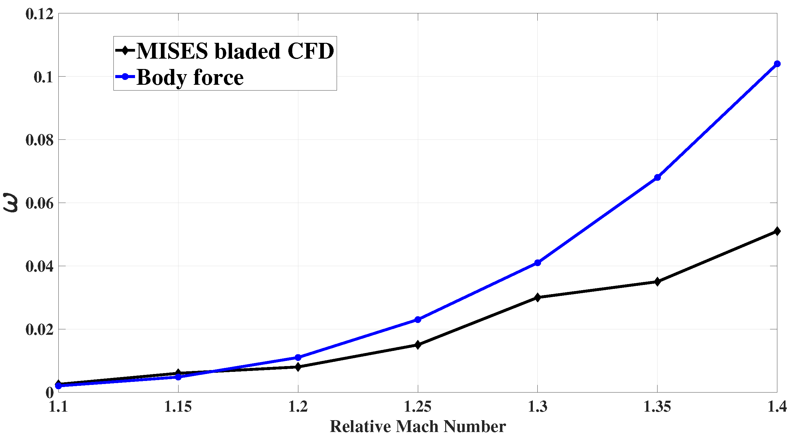
Finally, we assess the shock loss model introduced earlier. Figure 12 shows the shock loss coefficient computations in the body force and MISES for cascade 2. As expected, the model overpredicts the shock losses for high Mach numbers. To have a more accurate shock loss calculation, the normal component of Mach number incident to the shock wave should be used in the entropy generation equations [17]. However, in the body force modelling, the shock wave angle and its normal component Mach number cannot be determined. The model has an error of $25\%$ at a Mach number of 1.3. This error is acceptable as in a transonic rotor (as is shown in Ref. [25]), only in the outer $30\%$ span does the relative Mach number become greater than one such that shock losses come into the computations. Ref. [25] shows that a shock body force loss model is essential in predicting an accurate entropy generation in high speed compressors.

8. Conclusions

A new uncalibrated viscous body force model was introduced, by using the flow quantities from the trailing edge. Drela and Youngren’s loss model [24] was used as the base model. It was shown that when prescribing an accurate trailing edge momentum thickness into the simulations with the assumptions made, a good prediction in the loss model occurs. The new analytical momentum thickness equation performs well in compressors with geometries and flow conditions within the range of the training dataset. An example cascade whose geometry is outside the range of the ANN training data performed less accurately, with errors up to $27\%$. The approach is promising, enabling the use of body force models with no need for bladed RANS simulations. This should allow significant reduction in computational cost for accurate assessment of the efficiency impact of nonuniform flows, among other potential applications.

To expand on the scope of the current model, a full consideration of free-stream turbulence characteristics could be considered in future work. In addition, expanding the ANN training data to include higher camber values could help to improve the accuracy of the predictions for such blade sections. For the most aggressively cambered airfoils, many of the underlying model assumptions break down. To address this fully would require a local entropy generation-based loss model, incorporating local blade side velocities and boundary layer dissipation coefficients. This would require a loading model that predicts blade surface velocities instead of just the local loading. This is a difficult undertaking in highly three-dimensional flows.