1. Introduction
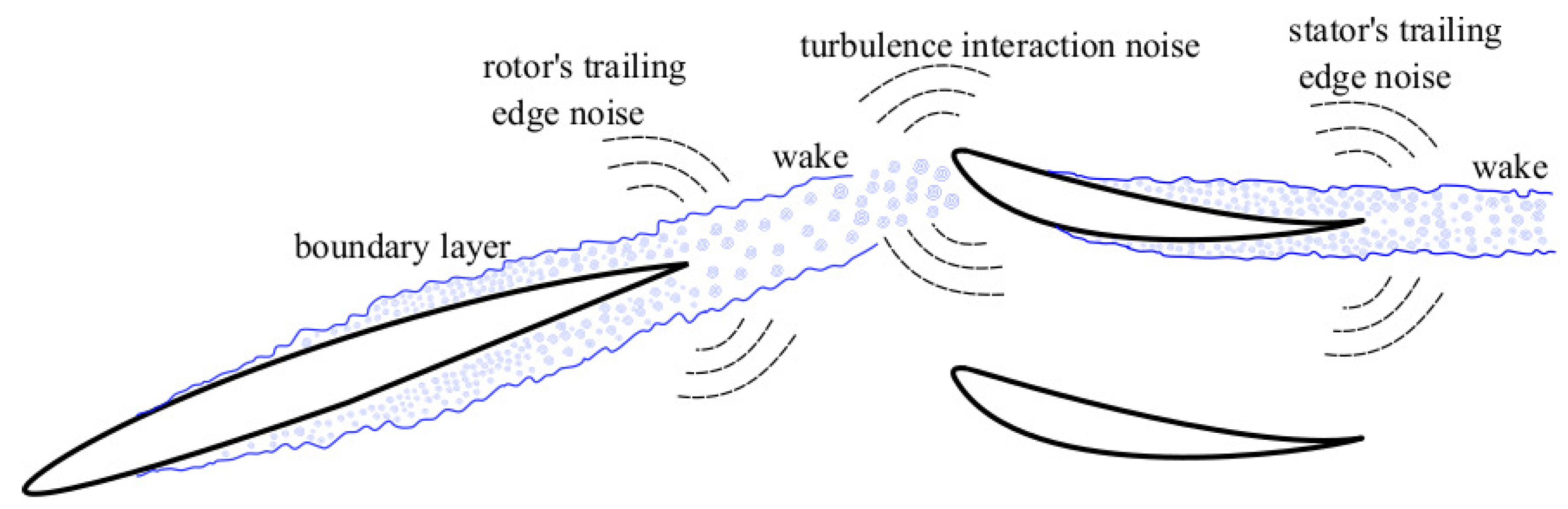
The increase in airports capacities and stringent noise regulations have turned noise pollution in the vicinity of airports into a significant challenge for aircraft manufacturers. In the last decades, jet noise has been significantly reduced by increasing the bypass ratio of turbofan engines. Additionally, the development of passive noise control technologies, such as acoustic liners and the use of convenient blade/vane counts have led to significant tonal noise reduction. Recently, modern ultra-high bypass ratio (UHBR) engines have allowed for further noise reduction while maintaining the fuel consumption reduction trend. Fan broadband noise becomes a major contributor to the total radiated noise. Thus, the understanding of the broadband noise has become a relevant research topic. Fan broadband from an aero-engine is generated by a number of mechanisms, such as turbulence ingestion, tip leakage vortex, rotor/stator self-noise, and turbulent fan wake impingement onto the outlet guide vanes (OGV). The last two mechanisms, also known as trailing edge noise (TEN) and turbulence interaction noise (TIN, or leading edge noise), respectively, illustrated in
Figure 1, are the object of the present numerical study.
Rotor broadband self-noise is generated by the scattering of turbulent kinetic energy from the boundary layer into acoustic waves as the flow encounters the singularity at the airfoil trailing edge. The estimation of airfoil self-noise requires an accurate prediction of the turbulent boundary layer development close to the trailing edge. For some airfoil configurations, at low to moderate Reynolds numbers, boundary layers may still be transitional as they reach the trailing edge. This is usually the result of large laminar flow regions around the airfoil, leading to self-sustained oscillations and Tollmien–Schlichting instability waves developing on the suction or pressure side of the airfoil. These waves may then interact with the trailing edge and generate additional noise. In order to study trailing edge noise at higher Reynolds numbers, such instabilities should be avoided. A possible solution to force the transition to turbulence is to trip the boundary layer [
1,
2].
The TIN results from a direct impingement of the rotor turbulent wakes on the stator leading edge. Turbulence coming from the rotor induces load fluctuations on the vanes, which produces broadband noise.
Different numerical approaches can be used to investigate airfoil broadband noise [
3,
4]. Direct numerical simulation (DNS) is convenient, as no turbulence modeling is required. However, it is still limited to simple cases due to its prohibitive CPU cost. The reduction in the computational cost requires the use of some level of turbulence modeling. In this work, large eddy simulation (LES) is used, in which only the smallest and poorly energetic turbulent eddies need to be modeled. The acoustic propagation can be directly resolved by LES. Alternatively, turbulent flow parameters can be extracted from LES to feed analytical broadband noise models.
The main objective of this paper is to investigate the numerical requirements for a correct description of the TEN and TIN mechanisms with LES. Comparisons to exact analytic models are preferred to avoid any experimental or numerical uncertainty in the reference data. Consequently, each noise mechanism is investigated separately on a dedicated flat-plate configuration. Flow conditions are chosen to be representative of the fan stage aero-engine at approach conditions with a significant chord-based Reynolds number () and a freestream Mach number of about . Beyond the investigation of the numerical parameters, this study is also the opportunity to clarify the dependency of broadband noise on the main physical parameters.
2. Analytical Models
The analytical models used in this study are based on Amiet’s work for single airfoils. The model assimilates thin airfoils, such as turbofan rotor blades or stator vanes, to flat plates with no thickness or camber and zero angle of attack.
Amiet’s TEN model [
5] describes the scattering of pressure fluctuations from an incident boundary layer at the sharp trailing edge [
6]. Assuming a large span to chord aspect ratio, the power spectral density (PSD) of the acoustic far-field, for an angular frequency
and an observer at (
,
,
), is given by
where
k is the acoustic wave-number,
,
c is the chord length,
L is the span length,
is the spanwise wave-number,
represents a convection-corrected distance, and
is the convective velocity.
is a statistical function related to the wall-pressure spectrum
slightly upstream of the trailing-edge, assuming homogeneous boundary layer turbulence.
is the associated spanwise correlation length
where
is the spanwise coherence between points separated by a distance
. In Equation (
1),
I is the aeroacoustic transfer function that can be considered as the sum of the contribution of the main scattering from the trailing edge
and the leading edge scattering correction
. Detailed expressions can be found in [
6].
The TIN model considered here was first proposed by [
7]. The incident wake impinging on the leading edge is assumed to be frozen turbulence and is described as a sum of spatial Fourier modes in the streamwise and spanwise directions. Assuming a large span to chord aspect-ratio, the resulting far-field sound at an observer position in the midspan plane (
,0,
) is given by
where
is the streamwise wave-number,
is the PSD of the upwash velocity fluctuations, and
is the total aeroacoustic transfer function. For a frozen turbulent velocity field
.
3. Trailing Edge Noise (TEN)
The simulations address the flow around a flat plate with a sharp trailing edge at a free-stream velocity
m/s, in atmospheric conditions (
kg/m
,
K,
Pa.s). The chord is
m and the thickness is equal to
. The Reynolds number based on the chord is Re
. The computational domain size is
in the
x-direction and
in the
y-direction. The spanwise extension is 10% of the chord length, which represents about five times the boundary layer’s thickness at the trailing edge. An additional simulation was performed with a span length equal to the chord length in order to assess the effect of confinement on the results. Unless mentioned otherwise, periodic boundary conditions are used in the spanwise direction. Non-reflective Navier-Stokes characteristic boundary conditions (NSCBC) [
8] are used at the inlet and outlet planes of the domain, as well as at the upper and lower boundaries. The AVBP explicit unstructured compressible LES solver developed at CERFACS [
9] is used to solve the governing equations, with the SIGMA sub-grid scale model [
10], and the two steps Taylor Galerkin TTGC scheme [
11], which is a third-order convective numerical scheme in space and time.
A parameter study is performed in order to study the influence of the near-wall modeling, the grid topology and refinement in the near-wall and wake regions, the spanwise domain extent and boundary conditions, and the tripping methodology. The nomenclature for the different cases is as follows:
[trip method]X[trip position]H[trip height]-[cell type][y]W[wake size]-[span BC/ extension]:
[trip method]: Geom or Source (defined in
Section 3.2);
[trip position]: position of the trip as a percentage of the chord from the leading edge;
[trip height]: height of the trip relative the boundary layer displacement thickness ;
[cell type]: near-wall cell type, P for prisms and T for tetrahedra;
[y]: value of at the wall. A value around 1 is used for wall resolved (WR) simulations, while larger values of indicate wall modeled (WM) simulations. In the latter cases, a simple wall model is used, with a dimensionless wall velocity for with and ;
[wake size]: cell size in the wake relative to the Taylor scale;
[spanwise BC]: PERIO for periodic (by default), SYM for symmetry;
[spanwise extension]: Sp0.1c and Sp1c for 10% and 100% of the chord, respectively.
For all the cases, the mesh is mostly composed of unstructured tetrahedral elements and is carefully clustered near the airfoil surface to achieve an adequate spatial resolution. Near the wall, two types of elements are compared: tetrahedral and prismatic. For the latter, 8 layers of prisms are superimposed. The smallest wall normal spacing corresponds to the first layer near the wall and increases progressively with a geometric ratio of 1:1. In all the cases, a square trip is used and the mesh around the geometric trip is tetrahedral in order to avoid very small cells, which would lead to inconveniently small timesteps.
3.1. Influence of the Mesh Type and Refinement at the Wall
The influence of the mesh type near the wall is studied by comparing tetrahedral and prismatic meshes. The trip height corresponding to H4 is used for this comparison since it gives the best transition in WM cases (as it will be shown in the next section).
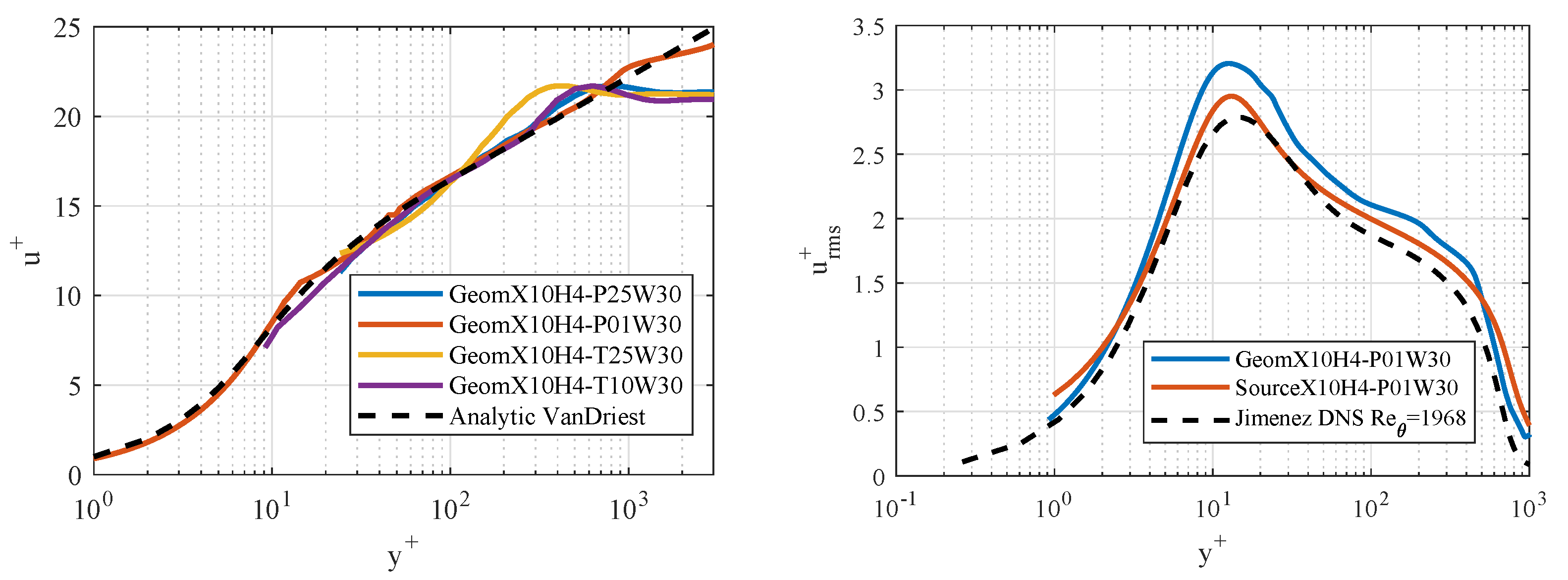
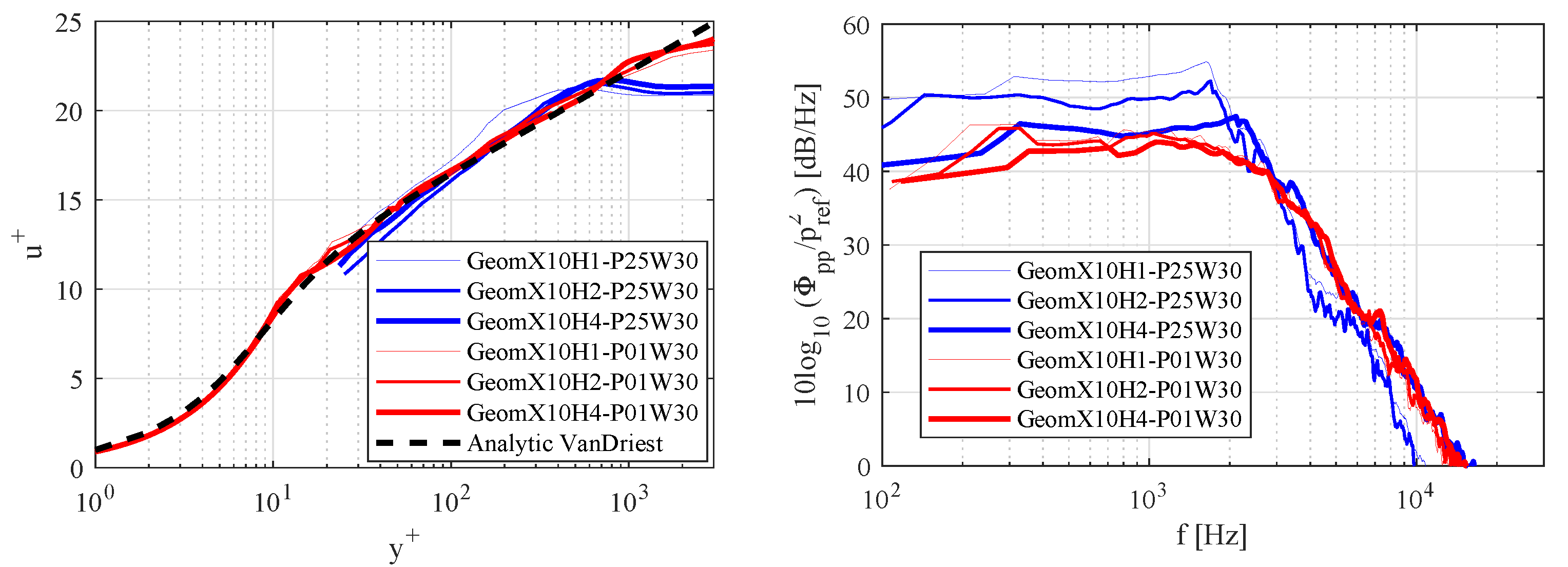
Figure 2 (left) shows
, the mean streamwise velocity
u normalized by the shear velocity
, as a function of the distance to the wall
, in wall units, at
. LES results are compared to the analytical solution of VanDriest [
12]. The WR case (GeomX10H4-P01W30) shows the best agreement as expected, with a slightly larger value of
in the buffer region when compared to the WM cases. In the WM cases, for the same value of
at the wall and the same CPU cost, a better agreement is found for the prismatic mesh when compared to the tetrahedral one. In order to reach a similar agreement, the tetrahedral mesh needs to be 2.5 times finer at the wall, which leads to
.
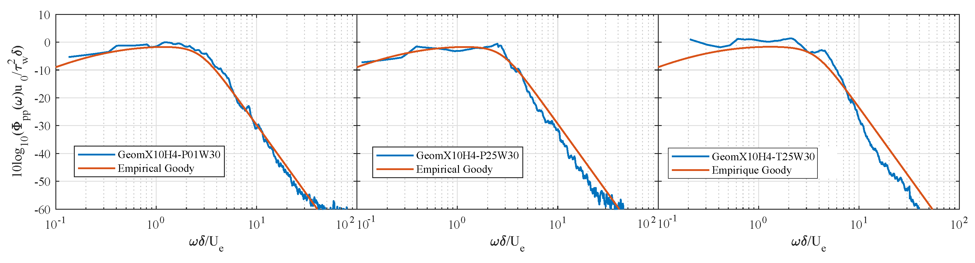
The influence of the mesh near the wall on the wall pressure spectrum (WPS) in the vicinity of the trailing edge is also analyzed.
Figure 3 shows the WPS obtained from the LES data, for prismatic and tetrahedral cases, compared to the empirical solution proposed by Goody [
13]. The numerical WPS are normalized by
and plotted against the reduced frequency
. It should be noticed that the WPS is quite sensitive to the mesh type and refinement close to the wall. A very good agreement with the empirical model is obtained in the WR case (GeomX10H4-P01W30), while some discrepancies can be found for the WM cases. For the tetrahedral case (GeomX10H4-T25W30), more discrepancies are visible, particularly at high frequencies.
3.2. Influence of the Tripping Methodology
Two tripping methods are compared in this study. The first one corresponds to a geometric trip on the plate surface, with a rectangular step shape, which requires a dedicated mesh. The second one involves a source term introduced in the streamwise momentum and energy equations, which has been designed to mimic the presence of a roughness element in the flow [
14]. The root-mean-square (RMS) velocity profiles
for the two tripping methods are compared in
Figure 2 (right) for WR simulations at a streamwise position corresponding to Re
(Reynolds number based on the momentum thickness of the boundary layer
). They are also compared to the DNS data from [
15]. Although the large geometric trip (“H4”) overestimates the turbulent intensity in the boundary layer, a very good agreement with the DNS data in terms of shape and amplitude is obtained using the source term. Thus, the source term allows for a correct transition without over-estimating the turbulence intensity.
3.3. Influence of the Trip Height
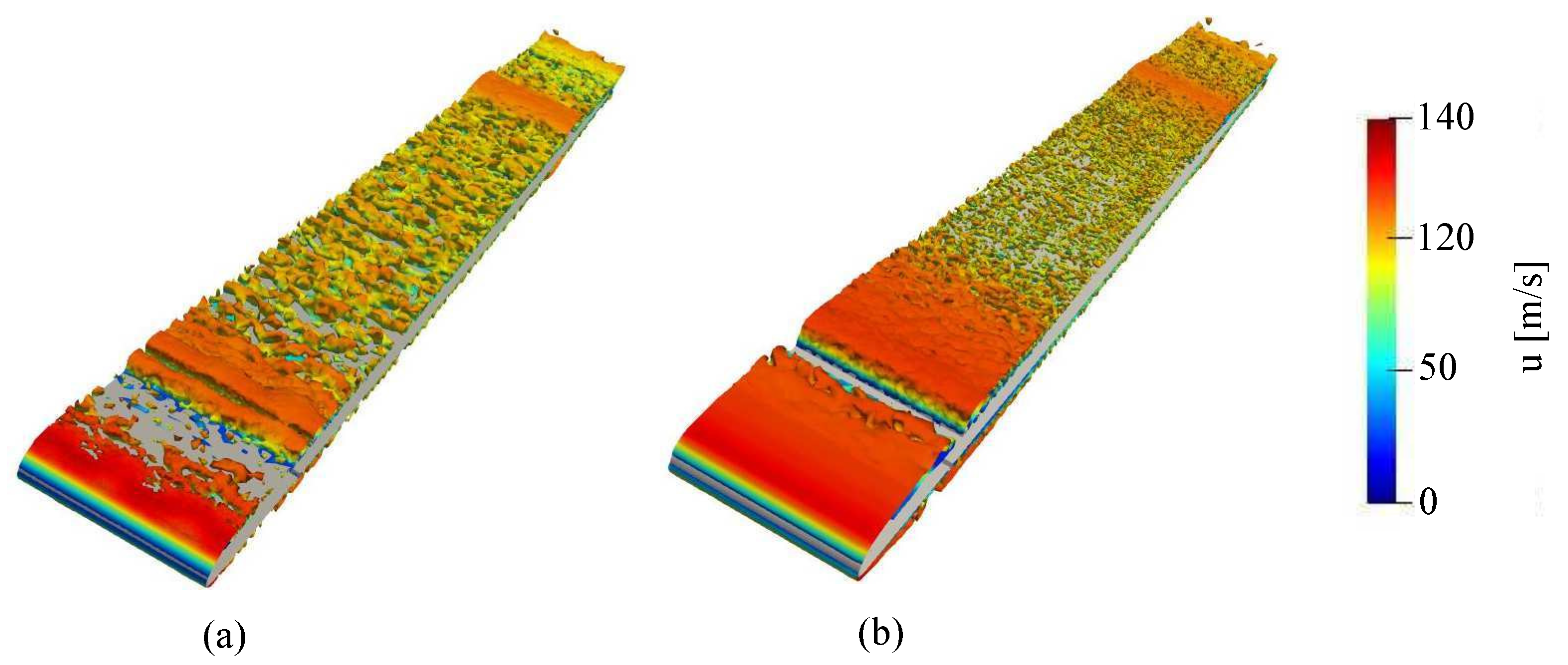
The influence of the trip height is studied in WM and WR cases. Three heights are considered for each case
= 1, 2, and 4. The instantaneous flow topology is shown in
Figure 4 for the trip heights H1 (a) and H4 (b) using iso-surfaces of Q-criterion from the LES computations. A transitional and turbulent boundary layer is found on both sides of the plate. The transition is triggered by the geometric trip with small structures appearing close to the reattachment point. Although similar turbulent structures are observed for both trip heights in the WR cases (not shown here), the WM simulation with the larger trip (H4) shows finer structures than that with the H1 trip. Note that for the WM cases, the small trip height (H1) is of the order of the first layer of prisms. The development of the turbulent boundary layer is then analyzed in
Figure 5 by comparing the normalized velocity profiles and the WPS near the trailing edge for the different trip heights. Identical velocity profiles are obtained for the WR cases with the three trip heights, in very good agreement with the analytical solution. However, as it can be seen in
Figure 5 (left) for the WM cases, the simulation corresponding to the largest trip “H4” shows a better agreement with the analytical solution. Thus, for WM simulations, the trip height must be sufficiently larger than the boundary layer displacement thickness in order to ensure an adequate boundary layer transition. This effect on the boundary layer transition can also be found by comparing the WPS profiles in
Figure 5 (right). Only slight differences are obtained between the WR cases. However, for the WM cases, the highest trip (H4) shows a reduction in the WPS amplitude by about 10 dB/Hz compared to H1 and H2 trips at low to moderate frequencies, but an increased intensity at high frequencies, and presents the closest spectrum to the ones obtained in WR cases.
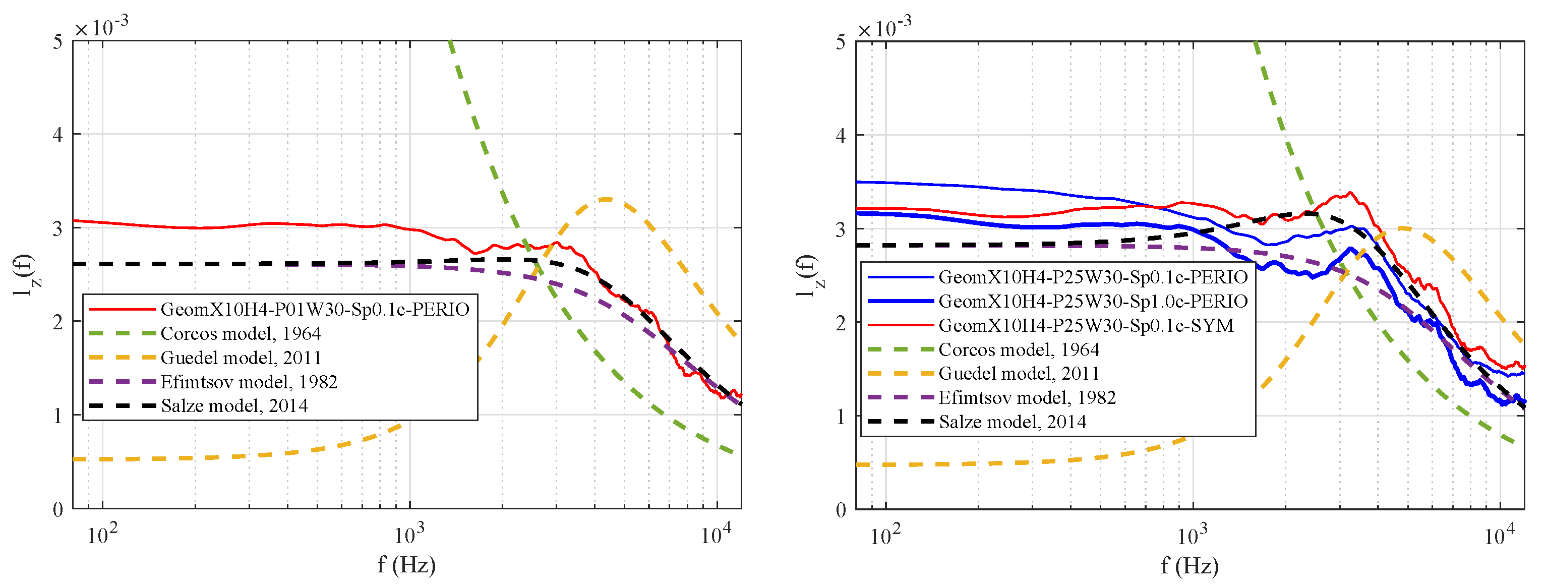
3.4. Influence of the Spanwise Extent and Boundary Condition
The influence of the spanwise extent and boundary condition on the spanwise correlation length
is examined in
Figure 6 (right) through a set of WM simulations corresponding to GeomX10H4-P25W30. Periodic (“PERIO”) and symmetry (“SYM”) boundary conditions are considered and two span extents (10% and 100% of the chord length) are investigated. In addition,
obtained from a WR case is given in
Figure 6 (left) as a reference. The LES results are compared to Corcos [
16], Guedel [
17], Efimtsov [
18] and Salze [
19] empirical models. Except for the models of Efimtsov [
18] and Salze [
19] that give slightly close results for
, large differences can be found with the other models. For the WR case, a good agreement with the model of Salze [
19] is observed for high frequencies and a slight over-prediction at low to mid frequencies is found due to the domain size. The model of Salze [
19] can, thus, be used as a reference for the WM cases.
Figure 6 (right) shows that periodic boundary conditions lead to a relatively better agreement with the model of Salze [
19] at high frequencies (
kHz) compared to symmetric boundary conditions, while a slightly higher over-prediction at low to mid frequencies can be noticed. When periodic boundary conditions are used, a perfect correlation is imposed between the boundaries, but the normal velocity fluctuations of turbulence are allowed. This explains why
is overestimated at low frequencies, which correspond to length scales of the order of the spanwise extent of the domain, and are correctly estimated at intermediate and high frequencies, which are mainly controlled by turbulence.
The comparison between the two span lengths is also showed in
Figure 6 (right). Even if the spanwise extent of the computational domain (
mm) appears sufficient when compared to the maximum correlation length (
mm), a larger extent improves the correlation length at lower frequencies. It can be observed that the spanwise correlation length
is significantly reduced, particularly at low and mid frequencies, when the large span is considered. The range where
is over-predicted is restricted to lower frequencies.
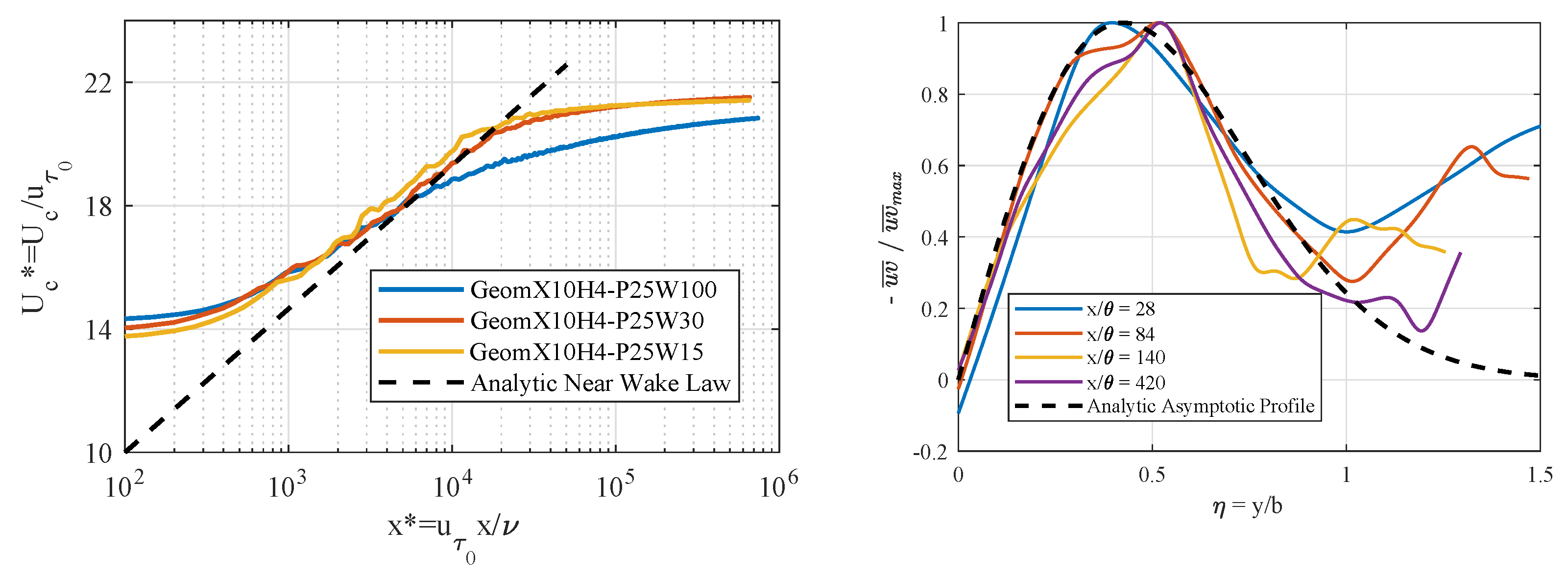
3.5. Influence of the Mesh in the Wake Region
For a fan/OGV stage, the wake formed behind the fan reaches the leading edge of the stator and generates rotor-stator interaction noise, which is the dominant source in such configurations. Thus, the numerical setup should allow for correct modeling and propagation of the fan wake in the inter-stage. After some distance downstream of the trailing edge of the fan blade, the wake reaches an asymptotic state. Once this length scale is known, the wake can be decomposed into three different regions: “near wake”, “intermediate wake”, and “far wake”. The asymptotic far wake stage is reached when all turbulent flow statistics follow universal distributions that are independent of the trailing edge conditions. Here, numerical results obtained from the LES cases are compared to empirical models or universal distributions in each wake region.
Three mesh refinements are considered in the wake region, denoted “W100”, “W30”, and “W15”. The WM case corresponding to the mesh type and refinement at the wall “P25” is used for all three cases.
Figure 7 (left) shows the streamwise development of the center-line velocity (
) for the three mesh refinements in the near wake region. The shear velocity
is computed at the trailing edge of the plate and the kinematic viscosity
is equal to its averaged value at each location. The LES results are compared with the near-wake analytic model proposed by [
20]:
where
,
,
, the function
g is defined as
, and
is the Euler-Mascheroni constant.
and
B are model constants equal to 0.418 and 5.5, respectively. It can be noted that beyond a certain streamwise position (
), a good agreement is found between the LES results and the analytical solution, although
is under-predicted for the coarsest mesh “W100”.
The intermediate wake characteristics are analyzed for the “W30” case by comparing the Reynolds stress profiles for different streamwise positions in
Figure 7 (right).
is the momentum thickness in the far-wake, with
U the longitudinal mean velocity, and
the constant freestream velocity outside the wake. In this region, the flow is expected to follow the asymptotic behavior given by [
20]
where
and
is the velocity deficit. The profiles are plotted against the normal coordinate
y normalized by the local wake half-width
b. For
, the normalized profiles are quite similar and fit well with the analytical solution. For larger values of
(i.e.,
), the analytical solution predicts a turbulent intensity that tends to zero, while the Reynolds stress from the numerical results approaches its value outside of the wake region.
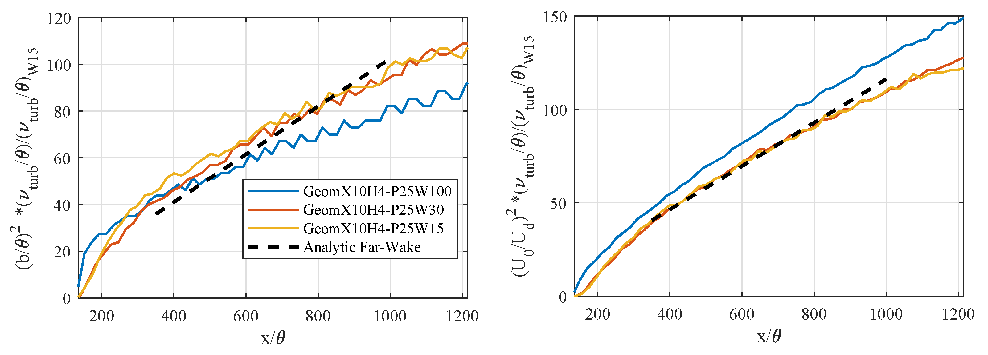
The far-wake properties are investigated in
Figure 8. The asymptotic behavior is reached approximately beyond
. The results in the far-wake can be compared to the half-power laws for the half-width
b and maximum velocity deficit
, which are given by
In the case of the refined meshes “W30” and “W15”, the power laws for
b and
are well predicted and the product
approaches the predicted constant value 0.9394 [
20]. For these cases,
approximately tends to 0.032 and
is slightly less than 0.0487 (see [
20]). The mesh resolution “W100” seems to be too coarse in the wake region. Thus, it can be concluded that the mesh resolution “W30” is sufficient to properly predict the flow in the wake region beyond a certain streamwise position, with an acceptable computational cost.
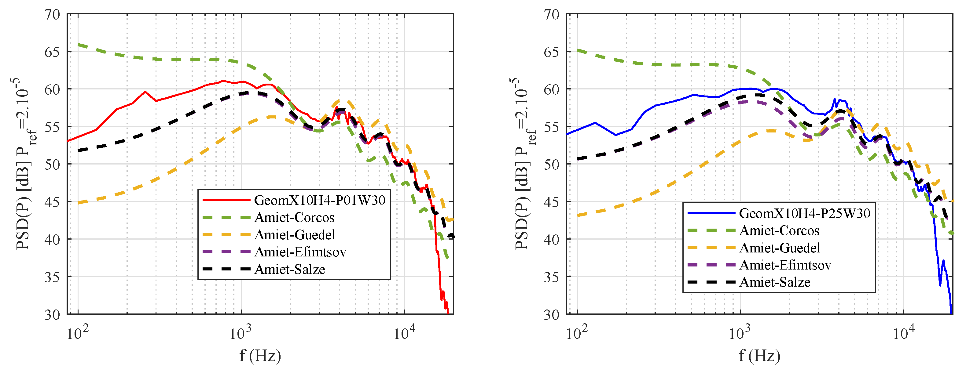
3.6. Acoustic Far-Field Predictions
The acoustic far-field predicted using the LES results from the GeomX10H4-P25W30 and GeomX10H4-P01W30 simulations (both providing 13 points per wavelength in the far-field and a total number of points of 3.1 and 13 millions, respectively) is compared to Amiet’s TEN model (see Equation (
1)). For the analytical predictions, the convection speed
is computed as the slope of the phase of the wall-pressure cross-spectrum between two streamwise locations in the vicinity of the trailing edge. The calculated values are between
and
. The wall-pressure PSD in the vicinity of the trailing edge
is extracted from the LES computation and is fitted to a Goody model, which can be used as an input in the TEN model. The spanwise integral lengthscale,
, is modeled using the analytical models shown in
Figure 6. For the direct numerical prediction, both the turbulent flow and the acoustic wave propagation are modeled by the LES solver. A comparison between the LES predictions and the analytical solutions of the PSD of the pressure fluctuations in the far-field, at 90° and a distance of
from the trailing edge of the plate, is shown in
Figure 9. The mesh cut-off frequency can be observed at around
kHz, the precise value depends on the mesh resolution. The analytical prediction is very sensitive to the model used for
. Both the WR and WM results show a good agreement with the model of Salze [
19] at mid-to-high frequencies, but seem to overestimate the low frequency levels. This can be explained by the domain confinement in the spanwise direction, as shown for
in
Figure 6.
4. Turbulence Interaction Noise (TIN)
Similar computational domain and numerical setup to the TEN simulations are adopted here. The only difference is related to the inlet boundary condition, where synthetic turbulence is injected, based on a summation of Fourier modes [
21]. The mean axial flow speed is
m/s. At a distance of
upstream the leading edge, the turbulent spectrum can be fitted to a Von-Karman spectrum with a turbulence intensity of 4% and an integral length scale of 5 mm (5% of the chord length). The cut-off wavelength is chosen as twice the largest cell size according to Shannon’s principle. The number of Fourier modes that compose the random velocity perturbation is 50. Turbulent kinetic energy follows the Passot Pouquet spectrum [
22].
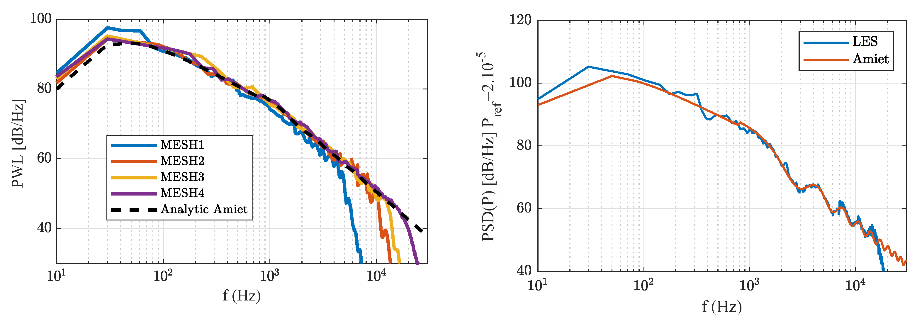
A total of four different grids are considered with 8 layers of prisms imposed on the plate surface. The mesh refinement at the wall is the same for all cases, and provide a consistent description of the RMS pressure along the plate (not shown). The only difference consists in the far-field cell size normalized by the chord length, equal to 1.7%, 2.1%, 3.6%, and 5.5% for MESH4, MESH3, MESH2, and MESH1, respectively.
Figure 10 shows the numerical power level spectra (PWL) for the different meshes at a distance of
(left), and the PSD of pressure fluctuations for MESH4 (right) for a probe at 90° above the plate leading edge. For comparison with Amiet’s TIN model, the PSD
and the spanwise correlation length
of the normal velocity fluctuations are extracted from the LES simulation slightly upstream of the leading edge and used as inputs for the model. Apart from slight differences at low frequencies, a very good agreement can be observed with the theory for all cases up to
kHz. All these meshes have the same structure and the same minimum cell size near the wall where the noise is generated. The far-field grid refinement influences the propagation and consequently the cut-off frequency of the spectrum, such that the most refined mesh can propagate a larger range of frequencies. One can infer from
Figure 10, for the specific numerical setup, that 13 points per wavelength are required to accurately capture acoustic waves up to a frequency of
kHz, which represents the audible limit. This valuable information will be used in the future to set up aeroacoustic-oriented LES simulations. Finally, it can be observed in
Figure 10 (right) that the numerical pressure PSD nicely reproduces the lobes of the analytical solution, which are due to the non-compact acoustic sources on the plate surface.
5. Conclusions
A parametric study on the effects of several numerical parameters on the flow development around a flat plate and the associated noise generation was conducted using LES simulations. The main noise mechanisms were investigated separately: trailing edge noise and turbulence interaction noise. The upstream flow properties and the geometric parameters of the plate were chosen to approach as close as possible the assumptions made in Amiet’s acoustic models. Comparison with analytical models and DNS data show very good results for the boundary layer characteristics and the far-field noise prediction. These results allow the definition of an adequate numerical set-up in order to prepare LES simulations of the broadband noise generated by an UHBR turbofan fan stage.
Author Contributions
Conceptualization, J.A.-A., V.C., A.G., J.B., and F.G.-A.; Data curation, J.A.-A.; Formal analysis, J.A.-A.; Funding acquisition, V.C., A.G., J.B., and F.G.-A.; Investigation, J.A.-A.; Methodology, J.A.-A.; Project administration, V.C., A.G., and J.B.; Software, J.A.-A.; Supervision, V.C., A.G., J.B., and F.G.-A.; Validation, J.A.-A.; Visualization, J.A.-A.; Writing—original draft, J.A.-A.; Writing—review editing, J.A.-A., V.C., A.G., J.B., and F.G.-A. All authors have read and agreed to the published version of the manuscript.
Funding
This work was performed within the framework of the industrial chair ARENA (ANR-18-CHIN-0004-01) co-financed by Safran Aircraft Engines and the French National Research Agency (ANR), and is also supported by the Labex CeLyA of the Université de Lyon, operated by the French National Research Agency (ANR-11-LABX-0060/ANR-16-IDEX-0005).
Institutional Review Board Statement
Not applicable.
Informed Consent Statement
Not applicable.
Data Availability Statement
Not applicable.
Acknowledgments
The computational resources were provided by GENCI (CINES, project number A0082A05039) and by FLMSN-PMCS2I at Ecole Centrale de Lyon.
Conflicts of Interest
The authors declare no conflict of interest.
Abbreviations
The following abbreviations are used in this manuscript:
| LES | Large eddy simulation |
| DNS | Direct numerical simulation |
| TEN | Trailing edge noise |
| TIN | Turbulence interaction noise |
| OGV | Outlet guide vanes |
| UHBR | Ultra high bypass ratio |
| PSD | Power spectral density |
| WPS | Wall pressure spectra |
| PWL | Power level |
| RMS | Root mean square |
| NSCBC | Navier-Stokes characteristic boundary conditions |
| TTGC | Two Steps Taylor Galerkin |
| WM | Wall-modeled |
| WR | Wall-resolved |
References
- Gonzalez-Martino, I.; Casalino, D. Noise from a Rotor Ingesting a Turbulent Boundary Layer Using Very-Large Eddy Simulations. In Proceedings of the 25th AIAA/CEAS Aeroacoustics Conference, Delft, The Netherlands, 20–23 May 2019; p. 2585. [Google Scholar]
- Winkler, J.; Wu, H.; Moreau, S.; Carolus, T.; Sandberg, R.D. Trailing-edge broadband noise prediction of an airfoil with boundary-layer tripping. J. Sound Vib. 2020, 482, 115450. [Google Scholar] [CrossRef]
- Lewis, D.; Moreau, S.; Jacob, M.C. Broadband Noise Predictions on the ACAT1 Fan Stage Using Large Eddy Simulations and Analytical Models. In Proceedings of the AIAA AVIATION 2020 FORUM, Virtual, 15–19 June 2020; p. 2519. [Google Scholar]
- Casalino, D.; Hazir, A.; Mann, A. Turbofan broadband noise prediction using the Lattice Boltzmann Method. AIAA J. 2018, 56, 609–628. [Google Scholar] [CrossRef]
- Amiet, R.K. Noise due to turbulent flow past a trailing edge. J. Sound Vib. 1976, 47, 387–393. [Google Scholar] [CrossRef]
- Roger, M.; Moreau, S. Back-scattering correction and further extensions of Amiet’s trailing-edge noise model. Part 1: Theory. J. Sound Vib. 2005, 286, 477–506. [Google Scholar] [CrossRef]
- Amiet, R.K. Acoustic radiation from an airfoil in a turbulent stream. J. Sound Vib. 1975, 41, 407–420. [Google Scholar] [CrossRef]
- Poinsot, T.J.; Lele, S. Boundary conditions for direct simulations of compressible viscous flows. J. Comput. Phys. 1992, 101, 104–129. [Google Scholar] [CrossRef]
- Schonfeld, T.; Rudgyard, M. Steady and unsteady flow simulations using the hybrid flow solver AVBP. AIAA J. 1999, 37, 1378–1385. [Google Scholar] [CrossRef]
- Nicoud, F.; Toda, H.B.; Cabrit, O.; Bose, S.; Lee, J. Using singular values to build a subgrid-scale model for large eddy simulations. Phys. Fluids 2011, 23, 085106. [Google Scholar] [CrossRef] [Green Version]
- Colin, O.; Rudgyard, M. Development of high-order Taylor–Galerkin schemes for LES. J. Comput. Phys. 2000, 162, 338–371. [Google Scholar] [CrossRef]
- Van Driest, E.R. Turbulent boundary layer in compressible fluids. J. Aeronaut. Sci. 1951, 18, 145–160. [Google Scholar] [CrossRef]
- Goody, M. Empirical spectral model of surface pressure fluctuations. AIAA J. 2004, 42, 1788–1794. [Google Scholar] [CrossRef]
- Boudet, J.; Monier, J.F.; Gao, F. Implementation of a roughness element to trip transition in large-eddy simulation. J. Therm. Sci. 2015, 24, 30–36. [Google Scholar] [CrossRef]
- Jiménez, J.; Hoyas, S.; Simens, M.P.; Mizuno, Y. Turbulent boundary layers and channels at moderate Reynolds numbers. J. Fluid Mech. 2010, 657, 335. [Google Scholar] [CrossRef] [Green Version]
- Corcos, G. The structure of the turbulent pressure field in boundary-layer flows. J. Fluid Mech. 1964, 18, 353–378. [Google Scholar] [CrossRef]
- Guedel, A.; Robitu, M.; Descharmes, N.; Amor, D.; Guillard, J.R. Prediction of the blade trailing-edge noise of an axial flow fan. In Proceedings of the Turbo Expo: Power for Land, Sea, and Air, Vancouver, BC, Canada, 6–10 June 2011; Volume 54648, pp. 355–365. [Google Scholar]
- Efimtsov, B.M. Characteristics of the field of turbulent wall pressure fluctuations at large Reynolds numbers. Sov. Phys. Acoust. 1982, 28, 289–292. [Google Scholar]
- Salze, É.; Bailly, C.; Marsden, O.; Jondeau, E.; Juvé, D. An experimental characterisation of wall pressure wavevector-frequency spectra in the presence of pressure gradients. In Proceedings of the 20th AIAA/CEAS Aeroacoustics Conference, Atlanta, GA, USA, 16–20 June 2014; p. 2909. [Google Scholar]
- Ramaprian, B.; Patel, V.; Sastry, M. The symmetric turbulent wake of a flat plate. AIAA J. 1982, 20, 1228–1235. [Google Scholar] [CrossRef]
- Smirnov, A.; Shi, S.; Celik, I. Random flow generation technique for large eddy simulations and particle-dynamics modeling. J. Fluids Eng. 2001, 123, 359–371. [Google Scholar] [CrossRef]
- Passot, T.; Pouquet, A. Numerical simulation of compressible homogeneous flows in the turbulent regime. J. Fluid Mech. 1987, 181, 441–466. [Google Scholar] [CrossRef]
Figure 1.
Schematic of trailing edge noise and interaction noise mechanisms for a fan/OGV stage.
Figure 1.
Schematic of trailing edge noise and interaction noise mechanisms for a fan/OGV stage.
Figure 2.
Mean and RMS velocities as a function of for different LES cases using different near-wall mesh type and refinements (left), and tripping methods (right).
Figure 2.
Mean and RMS velocities as a function of for different LES cases using different near-wall mesh type and refinements (left), and tripping methods (right).
Figure 3.
Wall pressure spectra (WPS) in the vicinity of the plate trailing edge (at 98% of the chord from the leading edge), for (left) GeomX10H4-P01W30 simulation, (center) GeomX10H4-P25W30 simulation, and (right) GeomX10H4-T25W30 simulation.
Figure 3.
Wall pressure spectra (WPS) in the vicinity of the plate trailing edge (at 98% of the chord from the leading edge), for (left) GeomX10H4-P01W30 simulation, (center) GeomX10H4-P25W30 simulation, and (right) GeomX10H4-T25W30 simulation.
Figure 4.
Iso-surfaces of Q-criterion (), colored by the velocity magnitude, for (a) GeomX10H1-P25W30 simulation and (b) GeomX10H4-P25W30 simulation.
Figure 4.
Iso-surfaces of Q-criterion (), colored by the velocity magnitude, for (a) GeomX10H1-P25W30 simulation and (b) GeomX10H4-P25W30 simulation.
Figure 5.
Comparison of the mean velocity profiles (left) and WPS in the vicinity of the trailing edge (right) between LES simulations using different trip heights.
Figure 5.
Comparison of the mean velocity profiles (left) and WPS in the vicinity of the trailing edge (right) between LES simulations using different trip heights.
Figure 6.
Spanwise correlation length, , for different spanwise boundary conditions (left), and different spanwise extents (right), in comparison with empirical models.
Figure 6.
Spanwise correlation length, , for different spanwise boundary conditions (left), and different spanwise extents (right), in comparison with empirical models.
Figure 7.
Comparison of the wake characteristics with empirical models in the near wake region (left) and the intermediate wake region ((right), for the computation GeomX10H4-P25W30, at different streamwise positions ).
Figure 7.
Comparison of the wake characteristics with empirical models in the near wake region (left) and the intermediate wake region ((right), for the computation GeomX10H4-P25W30, at different streamwise positions ).
Figure 8.
Asymptotic evolution of the wake’s parameters, for the three mesh refinements in the wake region, and comparison with the corresponding analytical solution.
Figure 8.
Asymptotic evolution of the wake’s parameters, for the three mesh refinements in the wake region, and comparison with the corresponding analytical solution.
Figure 9.
Direct prediction of the far-field PSD of pressure fluctuations from LES, in comparison to Amiet’s theory (various correlation laws), for an observer at and a distance of from the plate.
Figure 9.
Direct prediction of the far-field PSD of pressure fluctuations from LES, in comparison to Amiet’s theory (various correlation laws), for an observer at and a distance of from the plate.
Figure 10.
Comparison of the power spectral level PWL for the different meshes at a distance of (left) and the pressure PSD from the plate’s leading edge at a distance of for MESH4 (right) with the analytical solution of Amiet’s theory.
Figure 10.
Comparison of the power spectral level PWL for the different meshes at a distance of (left) and the pressure PSD from the plate’s leading edge at a distance of for MESH4 (right) with the analytical solution of Amiet’s theory.
| Publisher’s Note: MDPI stays neutral with regard to jurisdictional claims in published maps and institutional affiliations. |
© 2021 by the authors. Licensee MDPI, Basel, Switzerland. This article is an open access article distributed under the terms and conditions of the Creative Commons Attribution (CC BY-NC-ND) license (https://creativecommons.org/licenses/by-nc-nd/4.0/).


