
Modelling Turbine Acoustic Impedance †


Whittle Laboratory, University of Cambridge, 1 JJ Thomson Avenue, Cambridge CB3 0DY, UK
*
Author to whom correspondence should be addressed.
†
This paper is an extended version of our paper published in the Proceedings of the 14th European Turbomachinery Conference, Gdansk, Poland, 12–16 April 2021.
Int. J. Turbomach. Propuls. Power 2021, 6(2), 18; https://0-doi-org.brum.beds.ac.uk/10.3390/ijtpp6020018
Submission received: 10 May 2021
/
Revised: 1 June 2021
/
Accepted: 1 June 2021
/
Published: 7 June 2021
Abstract
:We quantify the sensitivity of turbine acoustic impedance to aerodynamic design parameters. Impedance boundary conditions are an influential yet uncertain parameter in predicting the thermoacoustic stability of gas turbine combustors. We extend the semi-actuator disk model to cambered blades, using non-linear time-domain computations of turbine vane and stage cascades with acoustic forcing for validation data. Discretising cambered aerofoils into multiple disks improves reflection coefficient predictions, reducing error by up to an order of magnitude compared to a flat plate assumption. A parametric study of turbine stage designs using the analytical model shows acoustic impedance is a weak function of degree of reaction and polytropic efficiency. The design parameter with the strongest influence is flow coefficient, followed by axial velocity ratio and Mach number. We provide the combustion engineer with improved tools to predict impedance boundary conditions, and suggest thermoacoustic stability is most likely to be compromised by change in turbine flow coefficient.
1. Introduction
Thermoacoustic instability is a coupling between unsteady heat release and acoustic waves in gas turbine combustors. If pressure and heat release fluctuations are in phase, the system is unstable and oscillations may grow to damaging levels. Prediction and hence mitigation of thermoacoustic instability requires acoustic impedance boundary conditions, characterising reflection of waves from the compressor and turbine back into the combustor. Reflected waves may arise from either incident pressure or entropy waves, so impedances for both cases are of interest. In computations of a realistic annular combustor by Lamarque and Poinsot [1], incorrect impedance boundary conditions yielded an error of 26% in the first resonant frequency.
The combustor outlet boundary condition is a function of turbine design. The state of the art for predicting the acoustic impedance of turbomachines is linear models based on the actuator disk approach of Cumpsty and Marble [2]. In the compact limit, , blade rows become a discontinuity in mean flow, and matching conditions based on conservation laws link incident and transmitted waves. Modelling multiple blade rows as a series of disks accommodates multi-stage turbomachines. For reduced frequencies typical of thermoacoustic instability, , waves require a finite time to propagate through blade rows. Kaji and Okazaki [3] relaxed the axially-compact assumption in their semi-actuator disk model, considering flat-plate cascades with finite chord, while assuming infinitesimal pitch to justify one-dimensional flow in blade passages.
Solving the full non-linear Navier–Stokes equations in the time domain is an alternative, more expensive method for predicting acoustic impedance. The only assumption in this approach is the validity of any turbulence closure used. Bauerheim et al. [4] use large-eddy simulations to validate the Cumpsty and Marble [2] actuator disk model for a two-dimensional turbine stage. The methods agree to within ±5% at low reduced frequency , but diverge at higher reduced frequency where the compact assumption is invalid.
Although actuator disk models have been demonstrated for specific cases, their negligible computational cost also makes them ideal for parametric studies. At present, there is no information available on the sensitivity of acoustic impedance to turbine aerodynamic design. This would be useful to a combustion engineer, allowing an assessment of possible thermoacoustic instability problems due to a turbine design change.
In this paper, we first extend the semi-actuator disk model to account for the cambered blades found in turbines. Next, we describe a time-domain computational fluid dynamics (CFD) approach for predicting acoustic impedance. Then, we compare predictions from the two approaches for a set of validation cases. Finally, we use the model to explore trends in acoustic impedance over the turbine design space. The contributions of this paper are:
- improvement of the accuracy of analytical models for turbine acoustic impedance;
- demonstration of an efficient CFD approach for predicting acoustic impedance; and
- quantification of the sensitivity of acoustic impedance to a complete set of aerodynamicparameters across the turbine design space.
2. Cambered Semi-Actuator Disk Analytical Model
We base our analytical model on the actuator disk approach developed by Cumpsty and Marble [2], and the semi-actuator disk method of Kaji and Okazaki [3]. Bauerheim et al. [4] present a comprehensive derivation of the actuator disk model, which we do not repeat here. In this section, we provide an overview of the basic theory and a description of our extension.
2.1. Mean Flow
The model treats unsteady, non-uniform flow as a perturbation to a specified steady, axisymmetric mean flow. Mean flow quantities take uniform values within each control volume, comprising the inlet, outlet, and spaces between blade rows as shown in Figure 1. For validation cases presented in this paper, we specify mean flow using time- and area-averaged CFD solutions. For the design space study, we specify mean flow using a one-dimensional mean-line solver with prescribed polytropic efficiency.
2.2. Characteristic Waves
Perturbations about the mean flow obey the two-dimensional linearised Euler equations in each control volume under the following assumptions:
- high hub-to-tip radius ratio, so spanwise variations are negligible;
- small amplitude perturbations, so products of perturbation quantities are negligible;
- high Reynolds number, so viscous and heat conduction effects are negligible.
For harmonic perturbations with a given frequency and circumferential harmonic, the general solution contains four arbitrary constants that set the perturbation flow field within each control volume. These correspond to four characteristic waves: upstream-running pressure, ; downstream-running pressure, ; convected vorticity, ; and convected entropy, [2]. To obtain a perturbation flow field, the task is to determine the amplitudes of these characteristic waves in all control volumes by applying boundary conditions.
2.3. Blade Row Modelling
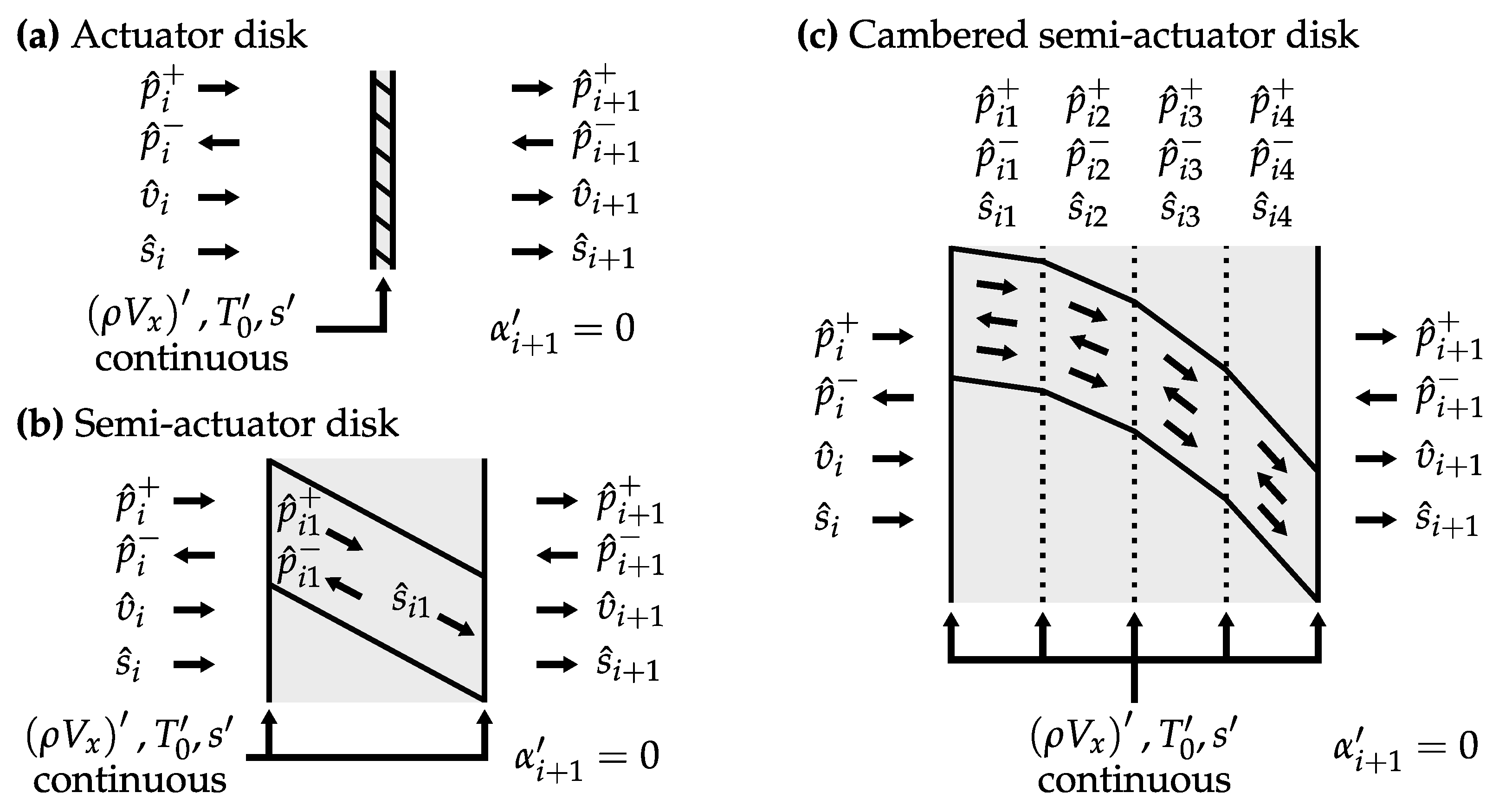
Enforcing continuity of perturbation mass flux, relative-frame stagnation temperature, and entropy across each blade row, combined with the Kutta condition , yields relations between characteristic waves in successive control volumes. Figure 2 illustrates applying these boundary conditions with varying degrees of fidelity. The result is always a system of four simultaneous linear equations for each blade row, which we express as a transfer matrix that yields a vector of characteristic waves in control volume on multiplication with the corresponding vector for control volume .
In the actuator disk approach, Figure 2a, blade rows are a discontinuity in mean flow, and matching conditions are independent of the flow inside the blade row. The semi-actuator disk approach, Figure 2b, captures axial non-compactness by treating blade rows as flat plates with finite chord. Assuming infinitesimal circumferential pitch, the flow is one-dimensional within blade passages, and the solution for harmonic perturbations inside the passage comprises pressure and entropy characteristic waves only. This neglects pitchwise non-compactness, but our results show it is an acceptable approximation in practice. Combining the matching conditions from leading and trailing edges, and eliminating the passage characteristic waves, gives the desired transfer matrix.
Turbine blades are highly cambered, unlike flat plates, leading to significant variations in mean flow along the blade chord. We account for this by discretising the camber line into multiple elements, Figure 2c, each with varying stagger angle. The flow is taken to be isentropic until the trailing edge, where the blade row loss is added. In the absence of detailed geometry data, we assume a quadratic camber line between inlet and exit flow angles. Applying the usual matching conditions between each element, and eliminating all passage characteristic waves from the resulting system of equations yields the row transfer matrix. In a typical case, the acoustic impedance becomes independent of the discretisation level for greater than 50 elements, the number we use in this paper.
2.4. Method of Solution
We use a superposition method to find perturbations that result from given boundary conditions at the turbomachine inlet and outlet. Downstream-running pressure, vorticity, and entropy waves are specified at the inlet, and two arbitrary guesses are made for the unknown upstream-running pressure wave. This completes a vector of characteristic waves in the first control volume, and successive multiplications by the blade row transfer matrices yield amplitudes in subsequent control volumes. The actual solution is the linear combination of both guess solutions satisfying the desired outlet boundary condition, of no upstream-running pressure wave in the final control volume.
3. Non-Linear Time-Domain Computations
This section describes a CFD-based approach to predicting acoustic impedances for a turbomachine subject to incident plane waves. We use a set of three simulations with different unsteady forcing about the same mean flow to determine impedances for incident pressure and entropy waves. The only inherent assumption is that the problem is linear. Implementation in an industrial-type CFD solver, with reflective boundary conditions and a second-order accurate discretisation scheme, results in a low computational cost compared to specialised high-order aeroacoustic codes. This is sufficient for the low reduced frequencies of interest.
3.1. Domain and Boundary Conditions
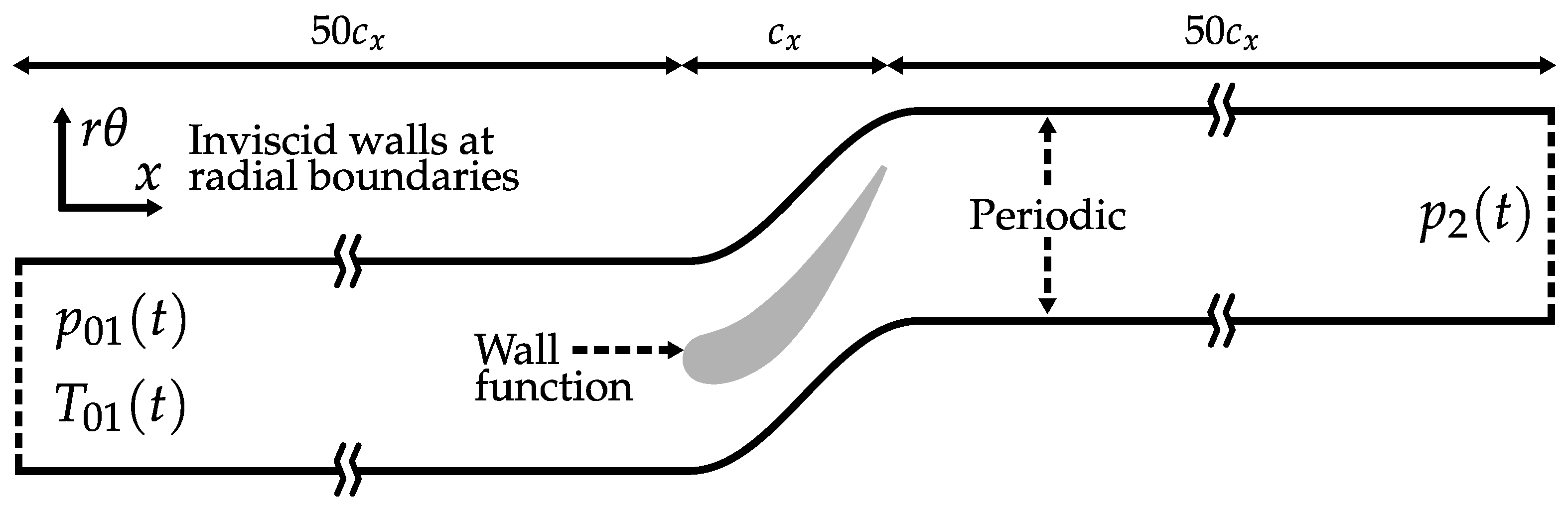
Figure 3 illustrates the computational domain and boundary conditions. Locating the inlet and outlet planes one wavelength of the fundamental forcing frequency (50 axial chords) away from the machine provides spatial resolution for wave separation. Inviscid walls at the radial boundaries enforce a two-dimensional flow. The time-averaged inlet boundary conditions are uniform stagnation pressure and temperature with no swirl, and the outlet boundary condition is a uniform static pressure.
We define unsteady perturbations to the boundary conditions using a forcing function,
where is the fundamental frequency, M is the number of harmonics, and is a small amplitude parameter. Three different forcing cases about the same steady operating point generate sufficient data to solve for acoustic impedance:
The boundary conditions are not non-reflective, and the imposed forcing is not in terms of characteristic waves. Therefore, each simulation will contain a linear combination of three cases with incident downstream-running pressure, upstream-running pressure, or entropy waves alone. Rather than attempting to simulate one of these ‘pure’ cases directly, we take the alternative approach of accounting for the combination effect in a post-processing step.
3.2. Post-Processing
We sample the unsteady flow field at a series of axial locations in the inlet and exit ducts, at least 10 axial chords away from the machine, and use this data to extract values for acoustic impedance. The post-processing method comprises the following stages:
- Area average. Area-averaging at each time step makes the unsteady flow at a given location spatially uniform, restricting the method to plane waves. Alternatively, applying constant-area mixed-out averaging (conserving mass, momentum, and energy) gives identical results;
- Fourier transform. Subtracting time-mean pressure and entropy from the instantaneous values at each axial location forms perturbations, which are transformed to the frequency domain using a fast Fourier transform algorithm;
- Wave separation. Applying the least-squares multi-microphone technique of Poinsot et al. [5] separates upstream- and downstream-running wave amplitudes from static pressure perturbations in the inlet and exit ducts;
- Reflectivity correction. We account for reflectivity of the computational boundary conditions using a ‘black-box’ technique after Emmanuelli et al. [6], first proposed by Cremer [7]. Expressing the wave amplitudes as a superposition of reflections, results for all three forcing cases form a system of six simultaneous linear equations. A matrix inversion yields the solution for the complex reflection and transmission coefficients.
3.3. Computational Details
All simulations in this paper were performed using turbostream 3, a multi-block structured unsteady Reynolds-averaged Navier–Stokes code developed by Brandvik and Pullan [8]. The spatial discretisation is second-order accurate finite-volume; the temporal discretisation is a second-order accurate dual time stepping scheme. A resolution study verified mesh independence with 45 points per shortest acoustic wavelength. There are 72 implicit time steps over the highest frequency of interest, and 500 explicit iterations converge each implicit step. We use the mixing length turbulence model, with a logarithmic-layer wall function at a distance in wall units. This assumes fully-turbulent boundary layers. In multi-row computations, an interpolation procedure matches the flow between grids in relative motion at rotor–stator interfaces.
A hub-to-tip radius ratio of 0.99999 approximates two-dimensional cascade geometry. The aerofoil section geometry is from the mid-span of a high-pressure turbine representative of a large industrial machine. Experimental data provide time-averaged boundary condition values.
We select a fundamental forcing frequency such that harmonics corresponds to a reduced frequency , representative of combustion instability. Forced unsteady simulations are started from a converged steady solution and run for 32 fundamental forcing periods before sampling flow field data over a further 32 periods.
4. Analytical Model Validation
In this section, we compare predictions of acoustic impedance from the analytical model to results from the CFD simulations. Agreement between the two independent calculation methods suggests that they are both valid. First, we demonstrate the benefit of a cambered actuator disk over a flat-plate treatment for a single turbine vane. Next, we quantify the effect of turbine cooling on acoustic impedance using simulations of a cooled vane with different coolant flow rates. Finally, we extend the methods to a turbine stage with stationary and rotating blade rows.
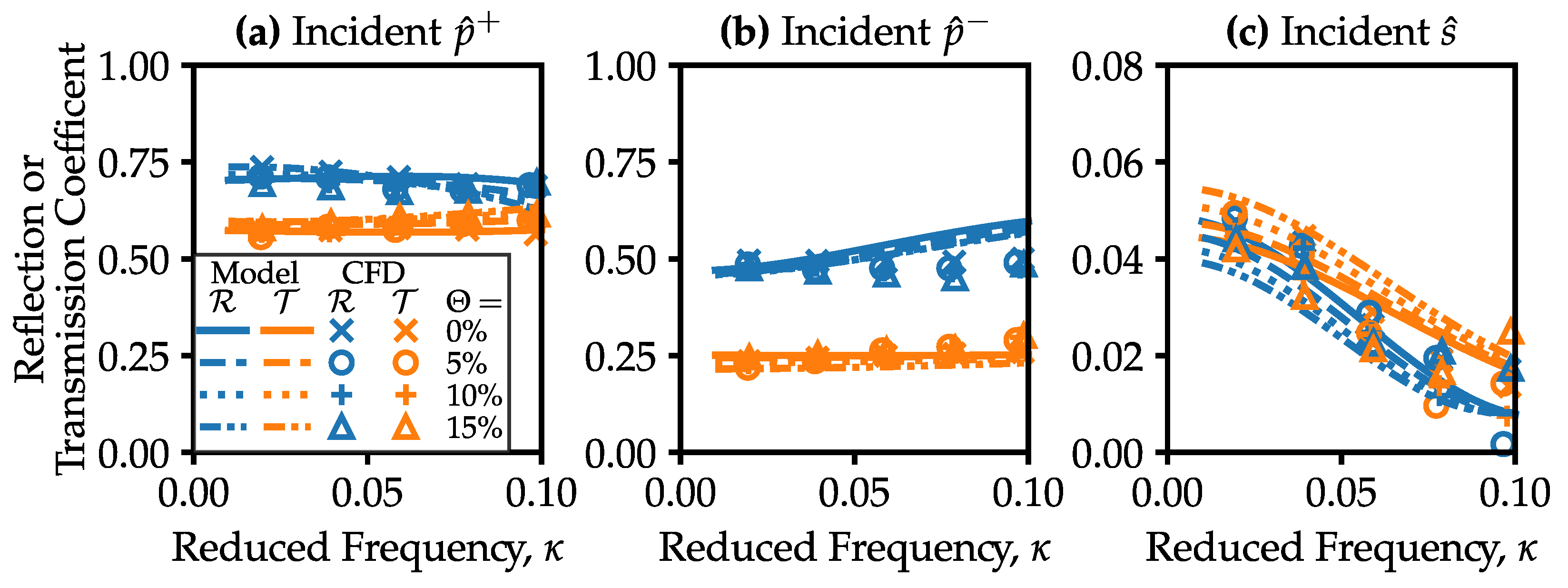
4.1. Uncooled Linear Vane Cascade
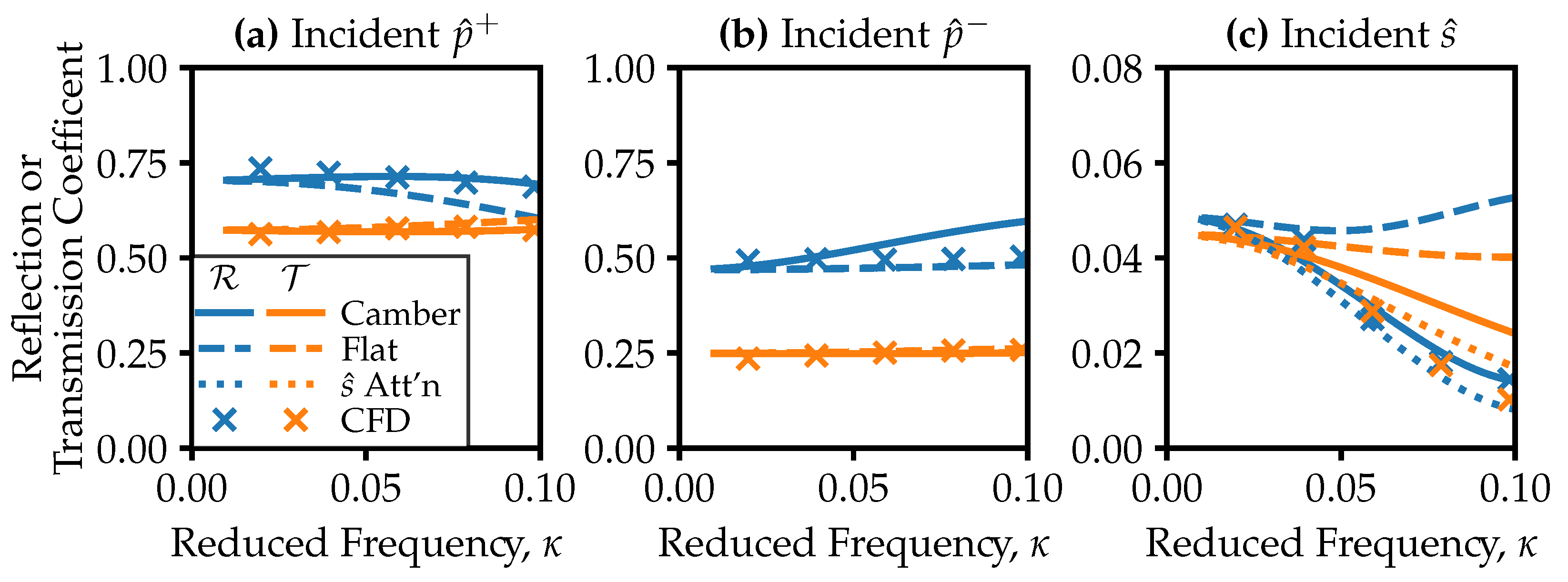
Figure 4 displays predicted acoustic impedances for an uncooled turbine vane, in terms of magnitudes of the (complex) reflection and transmission coefficients, and , as a function of reduced frequency, . Results for incident downstream-running pressure, upstream-running pressure, and entropy waves are shown in Figure 4a–c. We define the entropy wave coefficients as the entropy–acoustic transfer functions, suitably normalised: for example and .
We contrast two blade row models: a flat plate staggered at the mean of the inlet and exit flow angles, and a cambered vane. Both models converge in the zero-frequency limit, matching the CFD data to within ±5% at , but the flat-plate model fails to capture the trend with reduced frequency. At , the flat-plate model yields a 12% under-prediction of the reflection coefficient for downstream-running pressure waves, while the cambered model reduces this discrepancy to a 1% over-prediction, Figure 4a. For entropy–acoustic reflection, Figure 4c, the flat-plate model over-predicts by up to a factor of three, and the cambered model eliminates the error. Overall, the cambered model is a close match to the CFD for all reflection and transmission coefficients in Figure 4. The root-mean-square discrepancies between cambered model and CFD are ±2% for reflecting downstream-running pressure waves and ±11% for entropy–acoustic reflection.
The cambered model performs better because it accurately captures the time delay for waves to propagate through the blade row. Bauerheim et al. [4] note that the bulk convection time sets the slope of the entropy attenuation function at zero frequency. A flat plate with constant stagger angle does not account for axially non-uniform velocity within the blade passage, leading to a poor estimate of the bulk convection time. Bauerheim et al. [4] also show that higher-order frequency terms in the entropy attenuation function are due to entropy wave dispersion by circumferential velocity non-uniformity within the blade row. The neglect of this effect contributes to an over-prediction by our cambered model of transmitted entropy noise, by 140% at . Bauerheim et al. [4] accounted for entropy wave dispersion by tracing streamlines through a CFD solution of the blade row, and using time delays to calculate an attenuation coefficient. We use this approach for validation cases, where CFD solutions are available. Augmenting the present model with this technique, labelled Att’n in Figure 4c, reduces the over-prediction by half at . When CFD solutions are not available, however, the basic cambered model gives good predictions of entropy–acoustic reflection, the quantity of interest for thermoacoustic stability.
4.2. Cooled Linear Vane Cascade
In a typical gas turbine, film cooling controls metal temperatures below material limits. We model coolant flow in the computations using additional surface fluxes of mass, momentum, and enthalpy that reproduce the integral effect of film coolant ejection. In the analytical model, we represent cooling as a discontinuity in mean flow at the row trailing edge, together with the row loss, for simplicity. In principle coolant could be distributed along the camber line between the coupled semi-actuator disks.
We vary the coolant flow, , up to 15% of the inlet mass flow, a value representative of a highly-cooled nozzle guide vane (the exit Mach number is held constant). Figure 5 compares computational results and model predictions for the cooled vane. CFD data show that the variation in pressure wave reflection and transmission coefficients due to coolant flow is within ±3% of the mean over all coolant flow rates. The analytical model does not capture the trend with varying coolant flow rate: computations predict that acoustic impedance is independent of flow rate for , whereas the model predicts this to occur at . We attribute this to lumping coolant ejection onto the trailing edge in the semi-actuator disk model, while in reality film cooling alters the mean flow within the passage. The CFD shows increasing coolant flow tends to decrease reflected entropy noise, and the model agrees only qualitatively with this trend. Because of the relatively small effect size, and inaccuracy of the analytical model, we exclude coolant flow from our design space study.
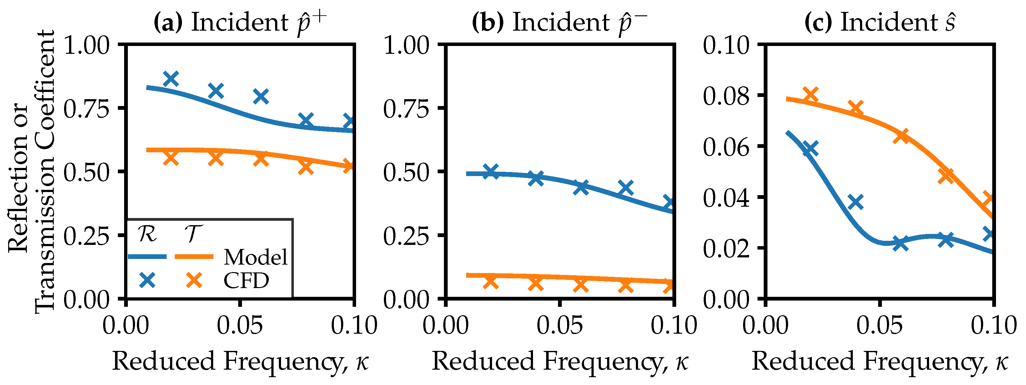
4.3. Linear Stage Cascade
Figure 6 compares acoustic impedance predictions for a two-dimensional, linear turbine stage cascade, using the cambered model and CFD. The analytical model captures the trends with reduced frequency, and is in good quantitative agreement with CFD simulations. The root-mean-square discrepancy is within ±7% for incident downstream-running pressure waves, and within ±16% for entropy–acoustic reflection. This confirms applicability of our methods for multi-row cases.
5. Design Space Study
In this section, we use the analytical model to map acoustic impedance across the turbine design space and quantify the sensitivity to aerodynamic design parameters. From dimensional analysis, the acoustic impedance of an uncooled two-dimensional turbine stage is a function of,
In gas turbines, the combustor imparts no swirl, so the stage inlet flow is axial, . The velocity triangles are controlled by: flow coefficient, ; stage loading coefficient, ; degree of reaction, ; and axial velocity ratios, and . These parameters are defined,
Textbook design practice is constant axial velocity, with . The maximum practical axial velocity ratio varies around the design space and corresponds to parallel annulus lines. The vane exit Mach number, , characterises density variations in the mean flow. Polytropic efficiency, , characterises stagnation pressure losses. We fix values of specific heat capacity ratio, , and reduced frequency, ; repeating the analysis with different values produces the same qualitative trends. We take the vane axial chord, blade axial chord, and axial spacing between the rows to be equal. Table 1 lists datum values for the parameters with representative upper and lower limits.
We generate families of turbine designs with different velocity triangles covering the classical Smith chart design space of intervals and , holding the other parameters constant at datum values. The cambered semi-actuator disk model predicts acoustic impedances for these designs subject to incident downstream-running pressure and entropy waves. Next, we perturb each of the other parameters in turn to determine their respective influences. Finally, we summarise by ranking the average sensitivity of acoustic impedance to all parameters.
5.1. Velocity Triangles
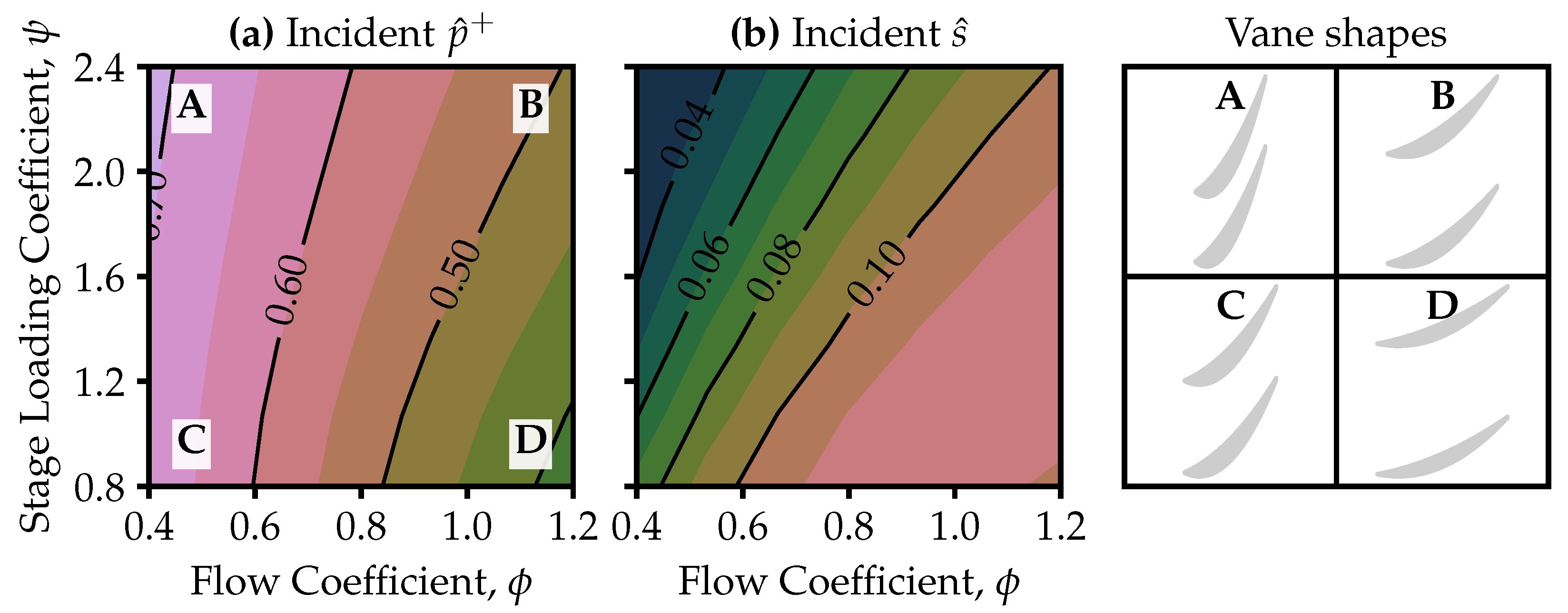
Figure 7 displays contours of reflection coefficients for turbine designs with , , , , and held at datum values, and illustrative vane shapes at the corners of the design space. Vane turning increases towards the top left of the chart: from Euler’s work equation .
For incident pressure waves, Figure 7a, the reflection coefficient is three times more sensitive to flow coefficient than stage loading coefficient. Increased aerofoil stagger angle produces greater acoustic impedance by geometric blockage [3], which leads to the highest reflection coefficient for high-turning designs. The blade speed Mach number scales rotational effects on the acoustic impedance; it reduces as stage loading increases, offsetting some of the rise in reflection coefficient due to increased turning. For incident entropy waves, Figure 7b, change in axial Mach number drives the trend in reflection coefficient. For constant vane exit Mach number, the axial Mach number and, hence, entropy–acoustic reflection is greatest for low-turning designs.
5.2. Other Parameters
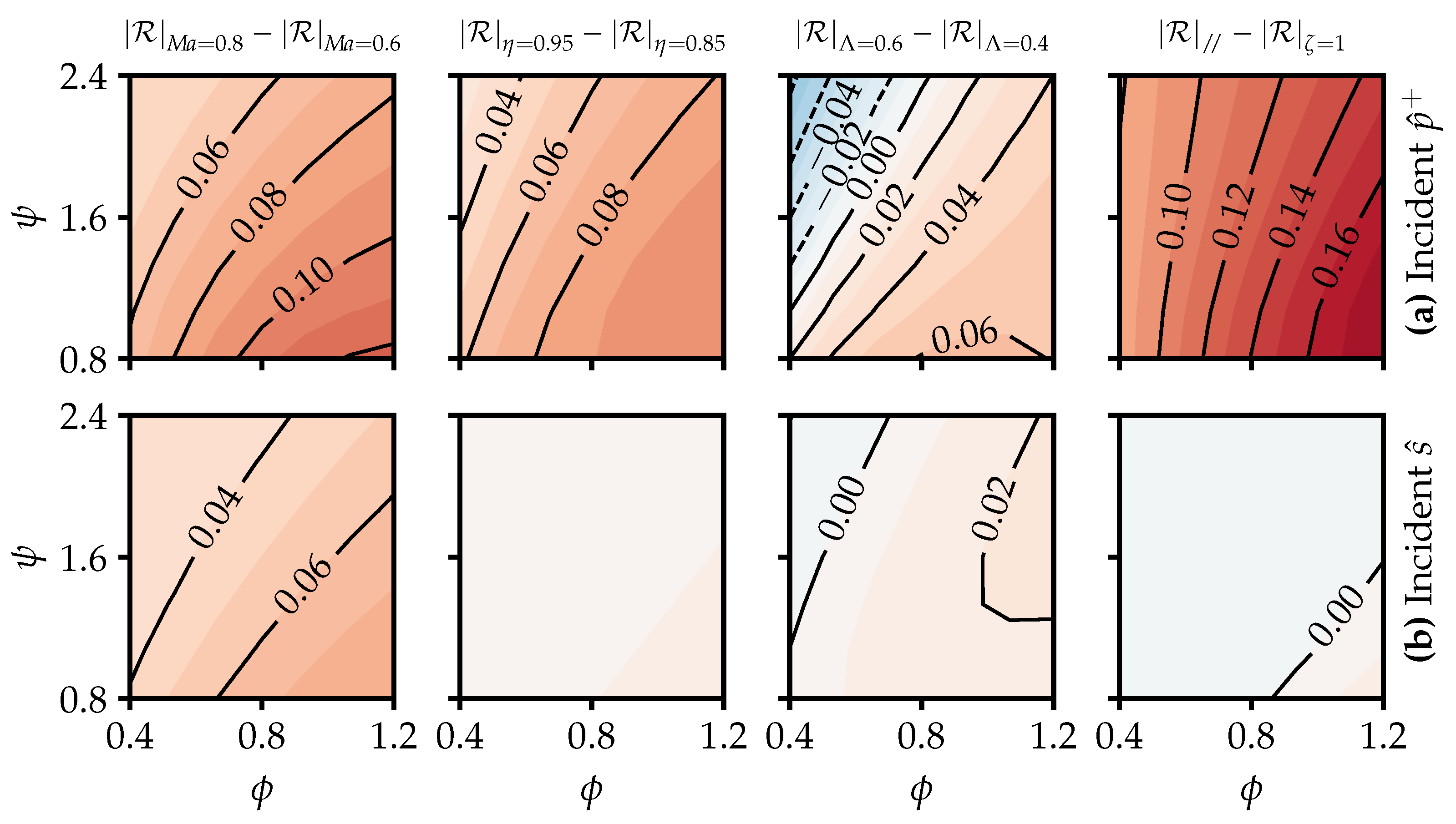
We now quantify the sensitivity of acoustic impedance to the parameters which were held constant in the preceding velocity triangle analysis. By repeating the calculations of Figure 7 changing one parameter at a time, and subtracting acoustic impedances at the upper and lower limits, we derive a directional sensitivity for each point in the design space. Figure 8a,b show results for incident pressure and entropy waves.
Increasing vane exit Mach number increases pressure-wave reflection coefficients, Figure 8a. The lowest-turning design is a factor of two more sensitive to vane exit Mach number than the highest-turning design. This is because lower flow angles imply a greater axial component of Mach number.
Varying reaction gives rise to two competing effects. First, it controls the balance of exit Mach numbers between vane and blade, with higher reaction leading to higher blade exit relative Mach number and increased reflectivity. Second, higher reaction reduces the vane loading and leads to lower vane exit flow angles, reducing reflectivity by geometric blockage. The latter effect dominates for high-turning designs, leading to a net reduction in reflection coefficient, and vice versa for low-turning designs, Figure 8a.
Changes in polytropic efficiency affect stagnation pressure loss through the turbine. As efficiency increases, less annulus divergence is required to keep Mach numbers and flow angles constant, and from Figure 8a the reflection coefficient increases. Less annulus divergence implies more contraction in flow area through each row, and, hence, increases reflectivity. Lower-turning designs, with less flow area contraction to begin with, are more sensitive to this effect, by a factor of two.
As with increasing efficiency, increasing axial velocity ratio leads to reduced annulus divergence, increased flow area contraction, and, hence, greater reflectivity, Figure 8a. Lower-turning designs are more sensitive because of their lesser existing contraction in flow area, as for polytropic efficiency. Highly-loaded designs are more sensitive because they produce greater density changes, requiring more annulus divergence to maintain constant axial velocity. Due to the combination of these effects, the sensitivity to axial velocity ratio is more dependent on flow coefficient than stage loading.
Now considering entropy–acoustic reflection, Figure 8b, the impedance is dominated by Mach number effects, with a maximum sensitivity of 0.08 for low-turning designs. This is consistent with a smaller rise of up to 0.03 in entropy–acoustic reflection coefficient for high-reaction, low-turning designs, due to increased rotor exit relative Mach numbers as discussed above. Varying polytropic efficiency and axial velocity ratio alters the entropy–acoustic reflectivity by less than 0.02.
5.3. Parameter Sensitivity Rankings
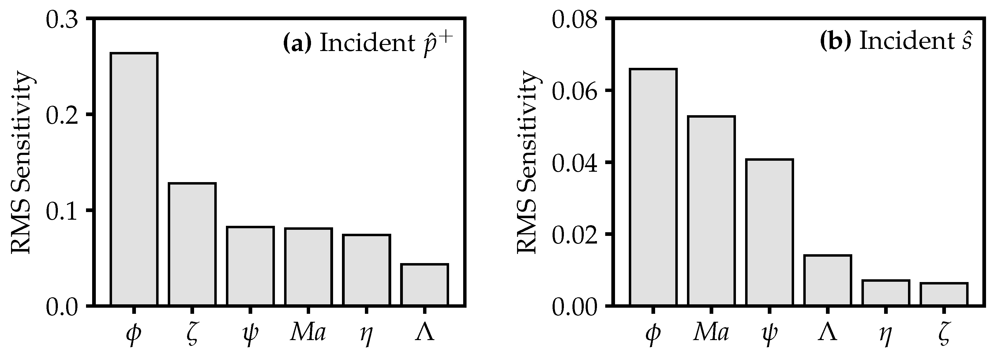
Figure 9 summarises the results of the design space study. We rank the parameters of Equation (3) in order of their influence on pressure wave and entropy–acoustic reflectivity. To quantify the average sensitivity to each parameter, we take the root-mean-square acoustic impedance change with respect to the datum value of that parameter.
Flow coefficient is the most significant parameter for pressure wave reflection, due to its influence on vane stagger angle, with a sensitivity twice that of the next parameter, axial velocity ratio. Flow coefficient is also of primary influence for entropy–acoustic reflection, with Mach number a close second. The influences of polytropic efficiency and degree of reaction are minor, with sensitivities less than 28% those of flow coefficient for both incident wave types.
So far, we have discussed only impedance magnitude results. Although we do not present the results here, we note that repeating the design space sensitivity study for impedance phase also yields similar rankings: flow coefficient, followed by stage loading are the most influential parameters.
6. Conclusions
- Predictions of turbine acoustic impedance using a cambered semi-actuator disk model agree with two-dimensional CFD simulations to within ±7% and ±16% for incident pressure and entropy waves, an improvement over simpler flat-plate models;
- For representative coolant flow rates, turbine cooling has a limited effect on acoustic impedance of ±3%. Increasing coolant flow rate reduces entropy–acoustic reflectivity;
- A parametric study of the turbine design space shows that acoustic impedance is most sensitive to flow coefficient, then axial velocity ratio, Mach number, and stage loading coefficient. Acoustic impedance is relatively insensitive to polytropic efficiency and degree of reaction.
Our work furnishes the combustion engineer with improved tools for efficiently and accurately predicting impedance boundary conditions, and the insight that thermoacoustic instability is most likely to be compromised by a change in turbine flow coefficient.
Author Contributions
Methodology, investigation, writing—original draft preparation: J.B.; supervision, funding acquisition, writing—review and editing: G.P. All authors have read and agreed to the published version of the manuscript.
Funding
This research was funded by Mitsubishi Heavy Industries, grant number G106034.
Acknowledgments
We thank Mitsubishi Heavy Industries for funding this project, and, specifically, Sumiu Uchida, Keijiro Saitoh, and Takaya Koda for their interest and support. We are grateful to Tom Hynes for sharing his semi-actuator disk code, and thank him for his helpful comments and suggestions.
Conflicts of Interest
We declare no conflict of interest.
Nomenclature
| Roman | Greek | ||
| a | Acoustic wave speed [] | Flow angle [] | |
| c | Blade chord [] | Specific heat ratio [–] | |
| f | Frequency [] | Polytropic efficiency [–] | |
| h | Specific enthalpy [] | Coolant flow fraction [–] | |
| Mach number [–] | Reduced frequency [–] | ||
| p | Pressure [] | Degree of reaction [–] | |
| Reflection coefficient [–] | Density [] | ||
| s | Specific entropy [] | Vorticity [] | |
| T | Temperature [] | Flow coefficient [–] | |
| Transmission coefficient [–] | Stage loading coefficient [–] | ||
| U | Rotor blade speed [] | Axial velocity ratio [–] | |
| V | Velocity [] | ||
| Subscripts | Accents | ||
| 0 | Stagnation conditions | Characteristic wave | |
| i | Control volume index | Perturbation relative to mean | |
| 1 | Vane inlet | Downstream-running | |
| 2 | Vane outlet | Upstream-running | |
| 3 | Blade outlet | Function of time | |
| x | Axial component | Time average | |
References
- Lamarque, N.; Poinsot, T. Boundary Conditions for Acoustic Eigenmodes Computation in Gas Turbine Combustion Chambers. AIAA J. 2008, 46, 2282–2292. [Google Scholar] [CrossRef]
- Cumpsty, N.A.; Marble, F.E. The Interaction of Entropy Fluctuations with Turbine Blade Rows: A Mechanism of Turbojet Engine Noise. Proc. R. Soc. Lond. 1977, 357, 323–344. [Google Scholar] [CrossRef]
- Kaji, S.; Okazaki, T. Propagation of sound waves through a blade row: I. Analysis based on the semi-actuator disk theory. J. Sound Vib. 1970, 11, 339–353. [Google Scholar] [CrossRef]
- Bauerheim, M.; Duran, I.; Livebardon, T.; Wang, G.; Moreau, S.; Poinsot, T. Transmission and reflection of acoustic and entropy waves through a stator–rotor stage. J. Sound Vib. 2016, 374, 260–278. [Google Scholar] [CrossRef] [Green Version]
- Poinsot, T.; Le Chatelier, C.; Candel, S.; Esposito, E. Experimental determination of the reflection coefficient of a premixed flame in a duct. J. Sound Vib. 1986, 107, 265–278. [Google Scholar] [CrossRef]
- Emmanuelli, A.B.; Huet, M.; Le Garrec, T.; Ducruix, S. Study of Entropy Noise through a 2D Stator using CAA. In Proceedings of the 2018 AIAA/CEAS Aeroacoustics Conference, Atlanta, GA, USA, 25–29 June 2018; p. 3915. [Google Scholar] [CrossRef]
- Cremer, L. The treatment of fans as black boxes. J. Sound Vib. 1971, 16, 1–15. [Google Scholar] [CrossRef]
- Brandvik, T.; Pullan, G. An Accelerated 3D Navier–Stokes Solver for Flows in Turbomachines. J. Turbomach. 2011, 133, 021025. [Google Scholar] [CrossRef]
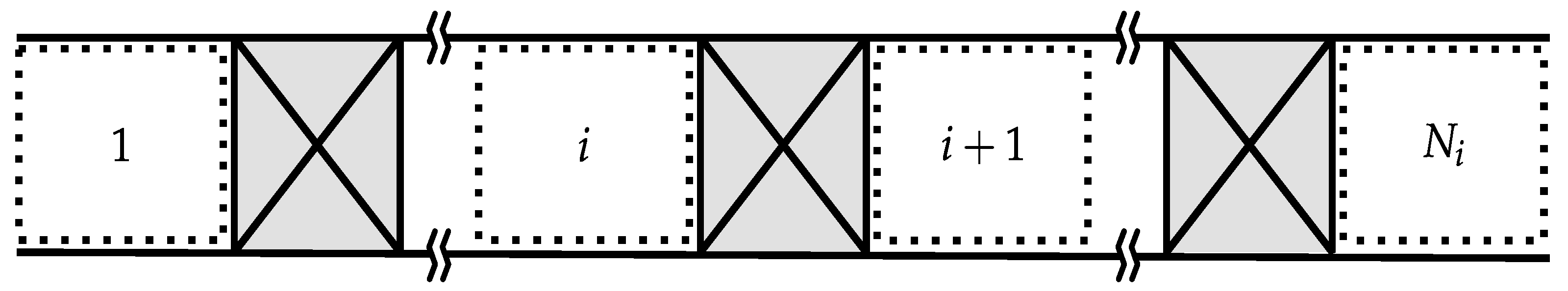
Figure 1.
Annulus control volumes in the semi-actuator disk model. The mean flow is uniform and steady over each of the inlet, outlet, and spaces between blade rows.
Figure 1.
Annulus control volumes in the semi-actuator disk model. The mean flow is uniform and steady over each of the inlet, outlet, and spaces between blade rows.

Figure 2.
Blade row models for determining acoustic impedance: (a) actuator disk, after Cumpsty and Marble [2]; (b) semi-actuator disk, after Kaji and Okazaki [3]; (c) our cambered semi-actuator disk.

Figure 3.
Domain and boundary conditions for computational fluid dynamics model.

Figure 4.
Reflection and transmission coefficients for an uncooled vane cascade, predicted by analytical model and CFD, for different incident characteristic waves. Att’n denotes augmentation with Bauerheim et al. [4] streamtube model. The cambered model matches the CFD results to within on average ±2% for downstream-running pressure wave reflection, and ±11% for entropy–acoustic reflection, an improvement over flat plates.

Figure 5.
Reflection and transmission coefficients for a cooled vane cascade, with varying coolant flow rates , predicted by cambered analytical model and CFD. The change in pressure wave reflection coefficients is small: within ±3% of the mean value over all flow rates.
Figure 5.
Reflection and transmission coefficients for a cooled vane cascade, with varying coolant flow rates , predicted by cambered analytical model and CFD. The change in pressure wave reflection coefficients is small: within ±3% of the mean value over all flow rates.

Figure 6.
Comparison of reflection and transmission coefficients for a two-dimensional turbine stage, predicted by cambered analytical model and CFD. The predictions agree on average to within ±7% for downstream-running pressure wave reflection, and ±16% for entropy–acoustic reflection.
Figure 6.
Comparison of reflection and transmission coefficients for a two-dimensional turbine stage, predicted by cambered analytical model and CFD. The predictions agree on average to within ±7% for downstream-running pressure wave reflection, and ±16% for entropy–acoustic reflection.

Figure 7.
Effect of velocity triangle design on acoustic impedance for incident downstream-running pressure and entropy waves. Pressure wave reflection coefficients are most sensitive to flow coefficient. Entropy–acoustic reflection increases for low-turning designs.
Figure 7.
Effect of velocity triangle design on acoustic impedance for incident downstream-running pressure and entropy waves. Pressure wave reflection coefficients are most sensitive to flow coefficient. Entropy–acoustic reflection increases for low-turning designs.

Figure 8.
Effect of secondary parameter variations on acoustic impedance, for incident downstream-running pressure and entropy waves. Contours of sensitivity calculated by subtracting acoustic impedances at the upper and lower limits of each parameter, with other parameters at datum values.
Figure 8.
Effect of secondary parameter variations on acoustic impedance, for incident downstream-running pressure and entropy waves. Contours of sensitivity calculated by subtracting acoustic impedances at the upper and lower limits of each parameter, with other parameters at datum values.

Figure 9.
Ranking of turbine design parameters by root-mean-square acoustic impedance sensitivity, for incident pressure and entropy waves. Flow coefficient is the most influential parameter.
Figure 9.
Ranking of turbine design parameters by root-mean-square acoustic impedance sensitivity, for incident pressure and entropy waves. Flow coefficient is the most influential parameter.


Table 1.
Datum values and upper and lower bounds for turbine design parameters.
| Parameter | , | |||||||
|---|---|---|---|---|---|---|---|---|
| Lower | 0.4 | 0.8 | 0.4 | — | 0.6 | 0.85 | — | — |
| Datum | 0.8 | 1.6 | 0.5 | 1.0 | 0.7 | 0.90 | 1.33 | 0.02 |
| Upper | 1.2 | 2.4 | 0.6 | parallel annulus | 0.8 | 0.95 | — | — |
Publisher’s Note: MDPI stays neutral with regard to jurisdictional claims in published maps and institutional affiliations. |
© 2021 by the authors. Licensee MDPI, Basel, Switzerland. This article is an open access article distributed under the terms and conditions of the Creative Commons Attribution (CC BY-NC-ND) license (https://creativecommons.org/licenses/by-nc-nd/4.0/).
Share and Cite
MDPI and ACS Style
Brind, J.; Pullan, G. Modelling Turbine Acoustic Impedance. Int. J. Turbomach. Propuls. Power 2021, 6, 18. https://0-doi-org.brum.beds.ac.uk/10.3390/ijtpp6020018
AMA Style
Brind J, Pullan G. Modelling Turbine Acoustic Impedance. International Journal of Turbomachinery, Propulsion and Power. 2021; 6(2):18. https://0-doi-org.brum.beds.ac.uk/10.3390/ijtpp6020018
Chicago/Turabian StyleBrind, James, and Graham Pullan. 2021. "Modelling Turbine Acoustic Impedance" International Journal of Turbomachinery, Propulsion and Power 6, no. 2: 18. https://0-doi-org.brum.beds.ac.uk/10.3390/ijtpp6020018