
Pulsed Flow Turbine Design Recommendations †


ISAE-SUPAERO, Université de Toulouse, 31400 Toulouse, France
*
Author to whom correspondence should be addressed.
†
This paper is an extended version of our paper published in the Proceedings of the 14th European Turbomachinery Conference, Gdansk, Poland, 12–16 April 2021.
Int. J. Turbomach. Propuls. Power 2021, 6(3), 24; https://0-doi-org.brum.beds.ac.uk/10.3390/ijtpp6030024
Submission received: 18 May 2021
/
Revised: 1 July 2021
/
Accepted: 6 July 2021
/
Published: 8 July 2021
Abstract
:A preliminary analysis of turbine design, fit for pulsed flow, is proposed in this paper. It focuses on an academic 2D configuration using inviscid flows, since pressure loads due to wave propagation are several orders of magnitude higher than friction and viscous effects do not significantly impinge on the inviscid part, as previously shown by Hermet, 2021. As such, a large parametric study was carried out using the design of experiments methodology. A performance indicator adapted to unsteady environment is carefully defined before detailing the factors chosen for the design of experiments. Since the number of factors is substantial, a screening design to identify the factors influence on the output is first established. The non-influential factors are then omitted in a more quantitative study of the output law. The surface response calculation allows determining the factor level favouring the best output. Consequently, the main trends in the turbine design driven by a pulsed flow can be stated.
1. Introduction
In many applications, the turbine is subject to temporal variations of its inlet conditions. The most extreme case is found when the turbine is involved in a thermodynamic cycle including the isochoric combustion process. During the last decade, the rising interest in aeronautics for isochoric combustion cycles has stimulated research on axial turbines supplied by severe unsteadiness. However, major contributions to this question are credited to the automotive turbocharger community. In Baines [1], a detailed summary of nearly 20 years of research on pulsed flow in radial turbines is given. This review highlights the progress and contradictions in the scientific community, particularly regarding the pulsed flow influence on turbine performance. The complexity of this problem comes from the coupling between different phenomenon involving time scales that are not easily separable (pulse time scale, propagative time scale, advective time scale, etc.). Moreover, the definition of a turbine performance indicator is made complex by this severe flow unsteadiness. This partly explains why there is no consensus on the pulsed flow influence in turbines, and more specifically whether or not the performance could benefit from the unsteadiness. The necessity to adapt the design process to the unsteady environment is increasing in the literature [2].
The complexity of the geometries involved in the different studies of the literature is also an additional difficulty to enlighten the comprehension. Recent numerical work [3] focused on that question through a simplified cascade approach. It has been shown that instantaneous loading differs from the quasi-steady approach in response to a rapid increase in turbine inlet pressure. The relevant time scale of the inlet perturbation associated with the additional work extracted by the turbine was also identified by the authors. In short, it appears that the curvature intensifies the different pressure effects during the wave propagation. Thus, a compression wave propagating in the direction of the flow overloads the blades, compared with a quasi-steady transformation. Other combinations of the nature of waves (compression or expansion) and the direction (upstream or downstream) have different consequences. For example, a streamwise expansion underloads the blades. In pulsating flows, a succession of waves of different natures and directions of propagation occurs. The net benefit of unsteady effects over a complete cycle thus needs to be quantified. It is one of the targets of this paper. However, the main objective is to give a clear statement on which geometrical parameters are likely to promote unsteady performance.
The present work is thus a direct continuation of the work of Hermet et al. [3]. The physics of pulsed flows is terribly complex. Therefore, the analysis is conducted by means of parametric studies for which the numerical design of experiments (DOE) is built. The adequate performance indicator is firstly discussed before describing the selected factors. Because of the large number of factors involved, an initial screening phase is conducted. This allows identifying the influence of each factor on the response. Noninfluential factors are then discarded for a more quantitative study of the output law. The quantitative prediction is built by calculating the response surface. As a conclusion, the main trends observed in 2D are exploited to propose first recommendations for the design of turbines able to benefit from the large unsteadiness of a pulsating flow.
2. Methodology
The parametric study focused on the simulation of stabilized pulsed flow through simplified cascade approaches of the stator and rotor with an in-house solver, forked from the solver [4]. is based on the resolution of the compressible formulation of the Navier–Stokes equations in their conservative form, spatially filtered, on an unstructured mesh using a finite volume method. An explicit third-order Runge–Kutta scheme was used for time advancement while an essentially non-oscillatory (ENO) second-order shock-capturing scheme was applied to compute the flux. The nonconformal and sliding interface, which develops between the rotor and stator domains due to the relative movement of the rotor and stator parts, was treated using a sliding mesh method based on the approach proposed by Bohbot et al. [5]. Such a methodology relies on the computation of geometrical intersections between the faces/edges located at the nonconformal interface and requires the reassessment of the parallel rank connectivity involved in the computation. The proposed sliding mesh method enables flux conservation across the interface and ensures accurate interpolations from cell to face averages by using information from cells and faces at each side of the interface. Moreover, the periodic properties of the solution were taken into account by duplicating the sliding interface geometry and solution data for each Runge–Kutta substep. Additionally, the grid motion was taken into account by means of the Arbitrary Lagrangian-Eulerian (ALE) [6] formulation, which allows solving conservation laws with moving grids in the absolute frame by adding specific flux terms to the discretized Navier–Stokes equations. The common face fluxes were computed following the Riemann HLLC solver adapted for moving grids [7]. Regarding the mesh grid density, a mesh convergence was performed on the first simulation of Table 1 to determine a reference density grid. For the other configurations, the number of points in the axial and normal direction was adapted in order to obtain the same density grid as the reference ones. Meshes were automatically generated by ICEM-CFD [8] using a script written in the Tool Command Language (TCL).
A stabilized pulsed flow is a perfectly periodic flow, similar to flows caused by the cyclic opening and closing of a valve separating the combustion chamber from the turbine. The choice of the performance criteria selected for the response of the DOE is first discussed. The selected factors of the design of experiments are then presented.
2.1. Response of the Design of Experiments
Most of the performance indicators used in the turbocharger literature do not take into account the full complexity of flow unsteadiness, as shown in [9]. In order to design a turbine under pulsed flow, the performance indicators of the turbine must be clearly defined. For this, it is appropriate to mention the mass conservation equation, as well as the first and second thermodynamic principles of an adiabatic unsteady system , Equation (1).
For stabilized pulsed flow (perfectly periodic), Equation (1) can be simplified by integrating over the inlet valve cycle duration. Actually, the temporal variations of the storage effects are cancelled out over the cycle. The system of Equation (1) then reduces to Equation (2).
From Equation (2), turbine performance indicators over a valve cycle can be defined. The aim of the paper is to give design trends that extract the maximum energy from the flow. It is then necessary to compare the energy extracted during a cycle to the energy injected into the turbine in a cycle; see Equation (3). When , the turbine extracts all the energy from the flow. This efficiency can be negative when flow waves cause a reversal in the direction of the aerodynamic force applied to the blades. In this case, the system operates as a compressor.
The indicator Equation (3) is not an efficiency as usually found in the literature and should not be considered as such. It corresponds to the output for the various factorial combinations considered in this paper, allowing a fair comparison among different pulsating profiles. It could be interpreted as a recovery coefficient. Now, the factors that may influence this output are described.
2.2. Factors of the Design of Experiments
The system design is not only based on the turbine geometry, but also on the inlet and outlet boundary conditions. In fact, the geometry allows extracting energy from the flow while the inlet and outlet boundary conditions (this is also the case of the geometry since it modifies the flow physics) contribute to creating favourable flow conditions for the work extraction.
2.2.1. Geometric Parameters
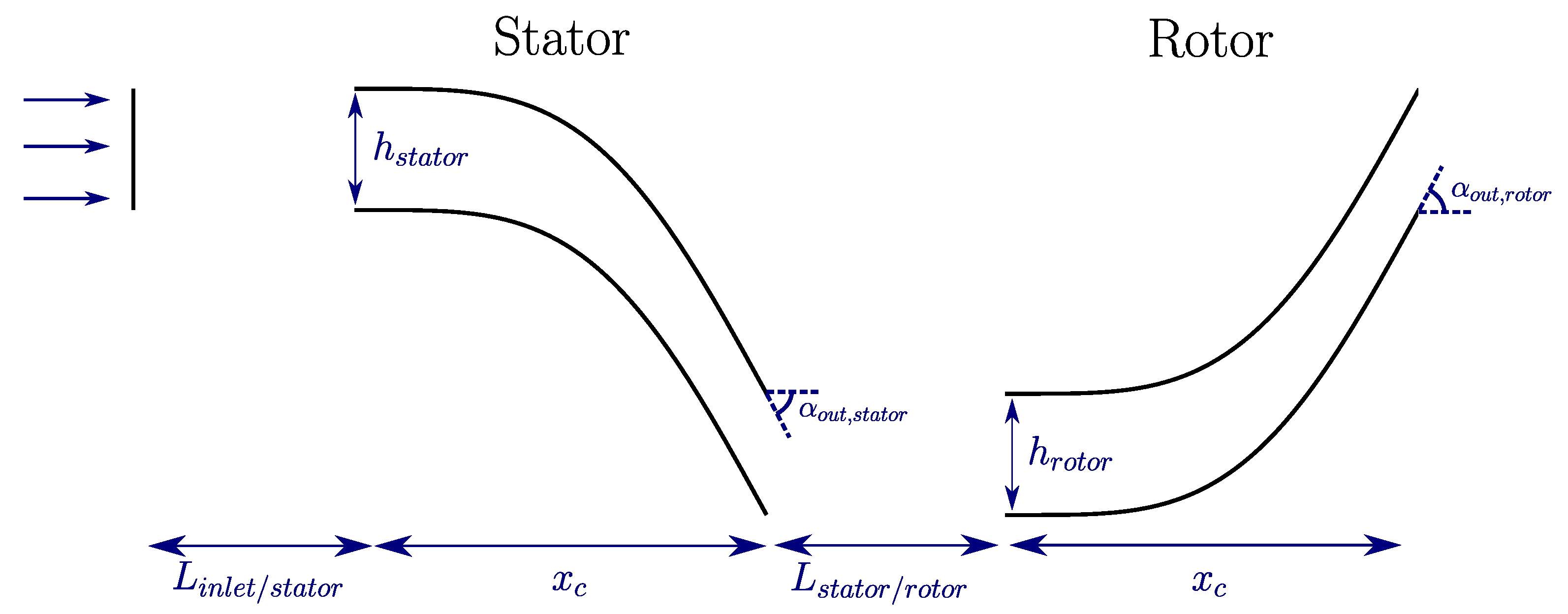
Several assumptions were made to reduce the number of geometric factors. First of all, the stator and rotor cascades were taken as thin and two-dimensional. Cascades were built with Equation (4). Angles at the leading edge of cascades in relation to the direction of the inlet flow were taken to be zero. Moreover, the axial lengths of the stator and the rotor blades were considered identical.
In addition to the blades’ geometrical parameters, the lengths between boundary conditions and the blades are significant for pulsed flows. They influence the location of the waves’ interaction in the domain. The length between the rotor trailing edge and the outlet boundary condition was considered very large to eliminate this parameter. The DOE geometric factors are shown in Figure 1.
2.2.2. Dynamic Parameters
The inlet valve cycle was chosen as a square wave. The opening and closing of the valve was instantaneous. During the opening phase, total pressure and total temperature were prescribed. A wall boundary condition was imposed during the closing phase. Under these assumptions, it took 4 factors to set up the valve cycle: , , and . To set up the simulation, an outlet pressure condition is applied: . The calculation information at the interface between the stator and rotor cascade was exchanged via a sliding mesh model, and rotor speed must be given: . The rotor speed was considered constant in the numerical simulations. The assumption was made that the valve cycles are much too fast for the rotor to adapt to the flow changes. All the other boundary conditions were supposed periodic.
2.2.3. Fluid Parameters
The analysed fluid was air. Thanks to the ideal gas law, the flow density is known. Only inviscid simulations were performed in this paper. Comparisons of large eddy simulations with inviscid simulations of transient flow within a 2D turbine cascade, carried out at the department [10], show that viscosity has no influence on the work prediction during the transient regime. No fluid parameter was added in the DOE factors.
2.2.4. Dimensionless Factors
The system behaviour law involves -dimensional parameters and fundamental units. Thanks to Vaschy–Buckingham’s theorem, the behaviour law can be determined with dimensionless parameters. The dimensionless factors of the design of experiments are listed in Table 2.
Most of the dimensionless factors are relatively easy to understand since they are usually used in steady-state flow turbines. However, some parameters, specific to pulsed flow, need to be specified. represents the cycle ratio, while and set, partly, the interaction wave locations. gives an indication about the distance travelled by a wave during . Indeed, is similar to the sound speed; thus, means that a wave propagating at the sound speed travels during .
The factor range of variation is also presented in Table 2. These ranges are large since the regions of the experiment domain that led to the best performance were unknown at the beginning of the study. The ranges were centred and reduced between and .
3. Results
3.1. Most Influential Factors
The design of experiments was built with the JMP® [11] software. To determine the factors’ influence on the output, a two-stage screening design was selected. This kind of design makes it possible to sort out from a large sample of factors those that have a non-negligible role on the system output and those that have little influence. These designs lead to a reduction in the dimensions of the factor space and a simplification of the problem. In this screening design, the level of each factor corresponds to the boundaries of the variation range, i.e., and as a coded variable. Consequently, the predicted output law is linear. The experimental design selected is a fractional factorial design. These designs are subsets of the full factorial designs. Fractional factorial designs are a good choice when resources are limited and the number of factors in the design is large; see [12] for more information. The simulations’ number of fractional designs was equal, here . The screening design is listed in Table 1.
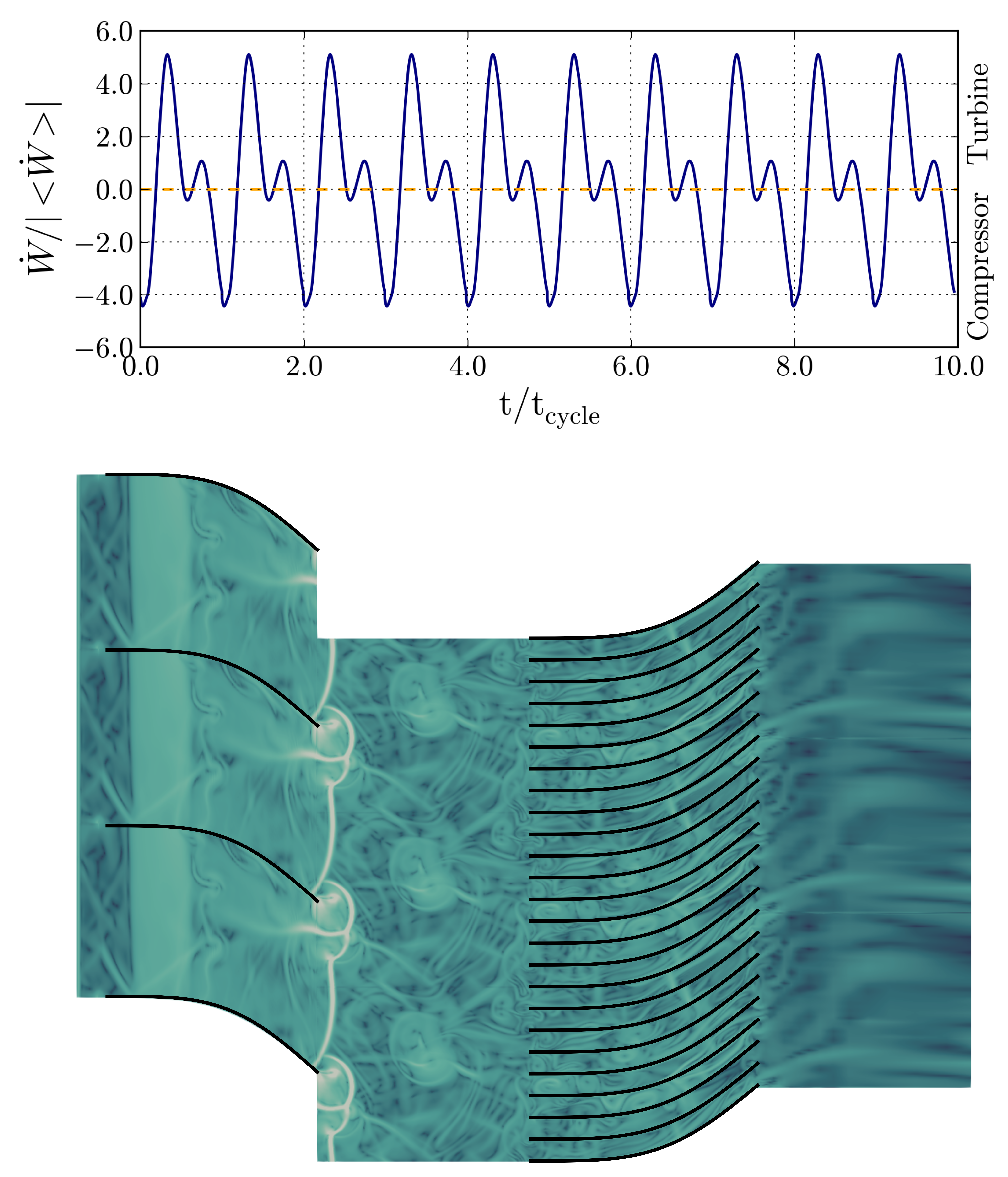
Screening design results are shown in Table 1. Two additional responses besides the recovery efficiency were proposed. Since the rotational speed is fixed, the strong decrease of mass-flow can make the compressor operating mode appear. The relative proportion of time in which this happens is quoted in %. Furthermore, the standard deviation of the work signal is reported in order to quantify the loading fluctuations. The recovery efficiency of many simulations is close to ; the turbine extracts almost no energy from the flow over a cycle. The system alternates between turbine and compressor phases. The balance between these modes is particularly visible on the temporal evolution of for the simulation in Figure 2. Compressor modes are driven by waves that generate a greater force on the suction side of the blade than on the pressure side. The temporal evolution of shows behaviours in agreement with the results of [3]. The valve opening causes a shock wave propagation, which generates a work increase. The valve closing generates an expansion wave, which causes a work decrease. An instantaneous visualization of the density gradient is also shown in Figure 2. This instantaneous visualization highlights the flow complexity.
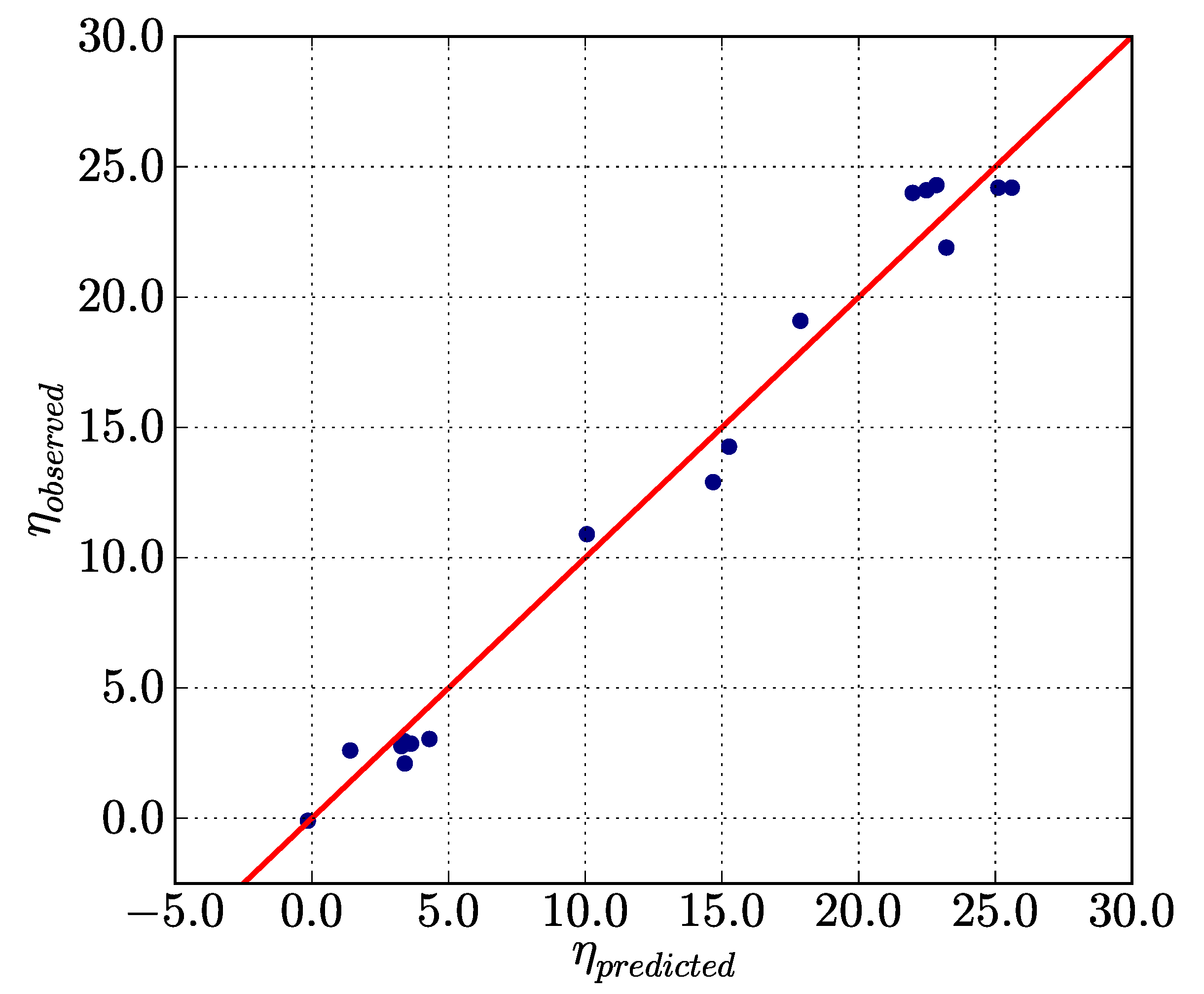
The linear prediction extracted from the screening phase is given in Figure 3. It shows a fair accuracy . Moreover, the distribution of the measured values in the observed performance range is relatively homogeneous, which gives confidence in the behavioural law prediction and legitimises the conclusions regarding the true influence of the different factors.
For the numerical experimental designs, the natural variability of the output can be considered as negligible. As a result, all factors in the design of experiments are statistically significant on the system output. However, some factors may be neglected by comparing the sensitivity values of the prediction model. A factor was considered to be noninfluential on the response when its sensitivity was less than of the maximum sensitivity of the model.
The sensitivity analysis showed that only six factors have a significant role in stage performance; see Table 3. The influence of these factors was further investigated by calculating the response surface. Understanding in detail why factors , , and do not influence the turbine recovery efficiency is difficult with such a flow complexity. However, the spatial distribution of the time-averaged energy recovered shows no sensitivity to these parameters. This result will not be presented here.
3.2. Surface Response
The reduction of the number of factors makes it possible to carry out a more quantitative study of the system output thanks to the response surface methodology [12]. The response surface modelling allows determining the factor that optimizes the output. For this design of experiments, the behaviour law prediction was performed by a quadratic function (see Equation (5)) with each selected factors.
In order to achieve a quadratic prediction of the output law, three levels for each factor must be considered in the simulations. In addition to the high and low levels , the central level 0 was added. For the calculation, the stator and rotor channels must be multiples of each other. The central value is then adjusted for and . The level of factors is indicated in Table 4. In the same way as the screening design, the experimental design was constructed using [11]. In order to minimize the simulations number, a D-optimality criterion was adopted for the design of experiments; see [12]. The surface response design was based on twenty-eight simulations for six factors. The levels of the noninfluential factors on the output, namely , , , and , were taken at their high level to carry out the simulations.
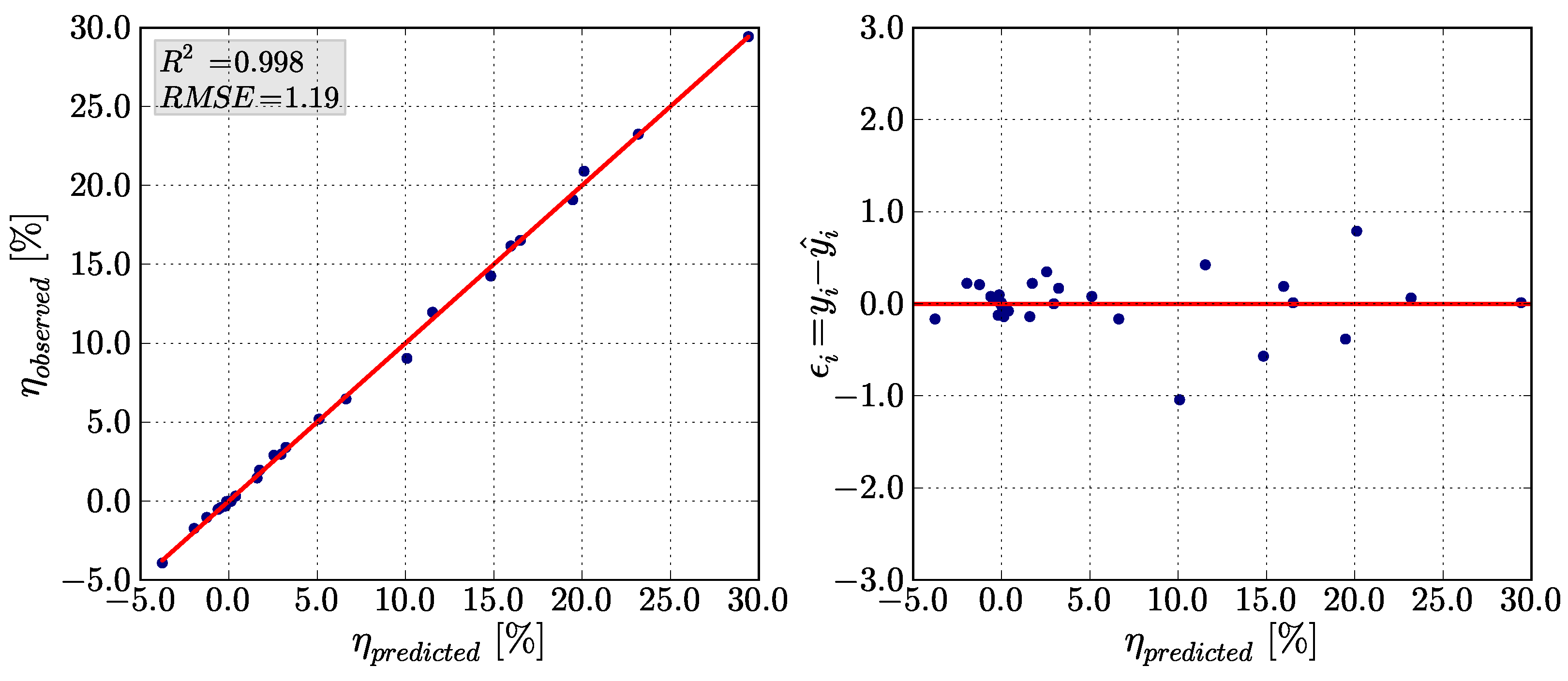
The results of the experimental design are provided in Table 5. The response surface accuracy can be examined by investigating Figure 4. It shows that the output law is very well modelled by the response surface . The spatial distribution of the measured values in the observed performance range is relatively homogeneous, which ensures that the predicted output law can be trusted. The model quality is also assessed on the residual value (Figure 4). The residuals are small and have no outliers.
It is interesting to focus on a few particular simulations showing original behaviours. Simulations or revealed that it is possible, with the wrong set of parameters, to design a system operating exclusively in compressor mode, whereas the target was to design a turbine. shows a fairly marked compressor mode over a cycle (13.5%), whereas this simulation leads to the highest recovery efficiency observed.
The factor levels that optimize the response are shown in Table 6. The maximum efficiency in the experimental domain is . The result on the coded variables reveals that the real optimum of this system is outside the experimental domain. Indeed, except for , the optimal value of the factors is located on the boundary of the experimental domain. This is promising since it means that it is possible with this system to extract more than of the injected energy into the turbine over a valve cycle, if the experimental domain is redefined in order to find the global optimum. For comparison, the value calculated for the usual turbofan is about for the high-pressure turbine stage ( K, K).
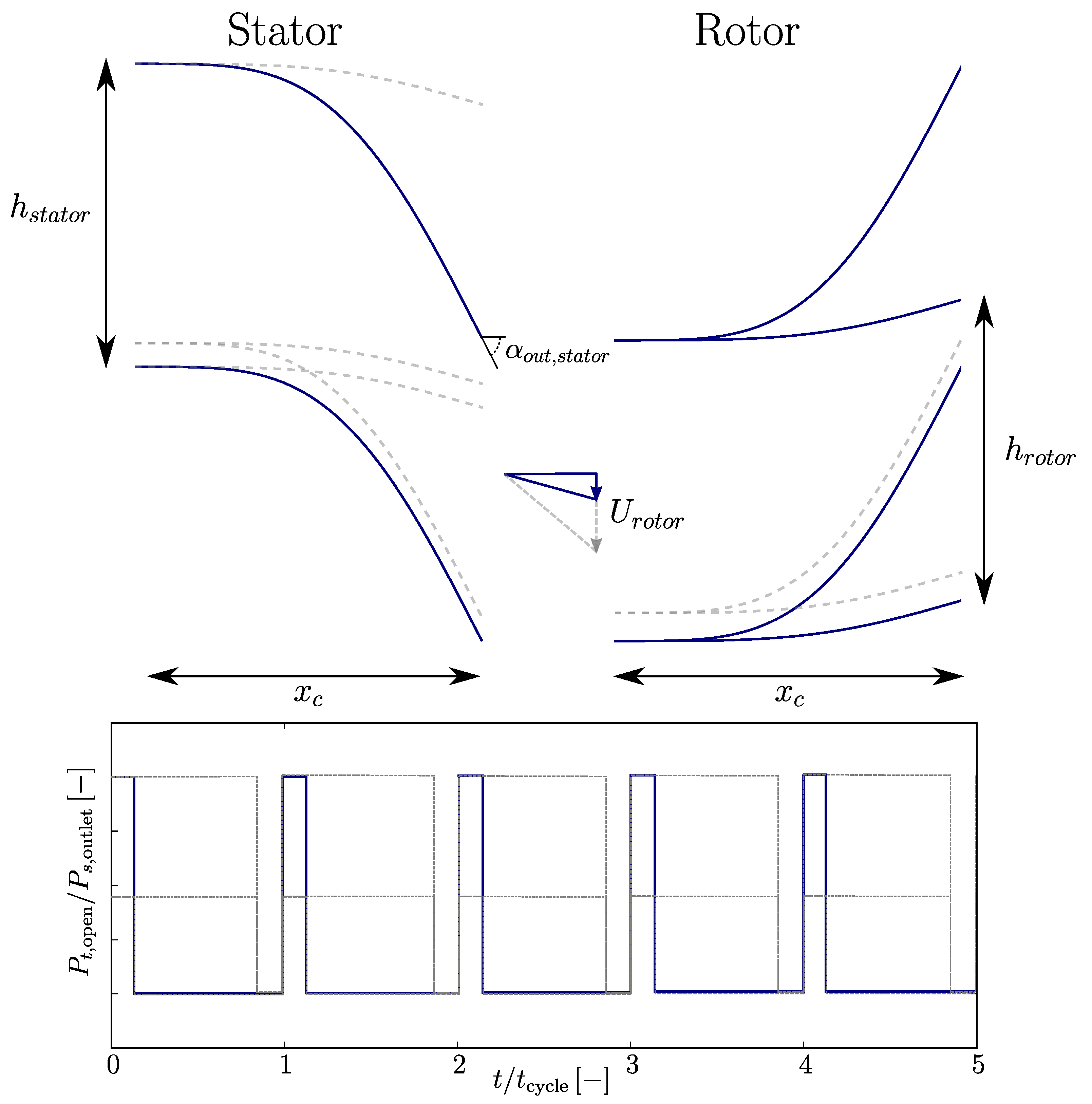
The position of the optimum gives the main trends for the design of a turbine fed by a pulsed flow, as far as 2D analysis can be applied. It reinforces the usefulness of the stator for this system. This result was not evidence since the instantaneous performance is dictated by the waves’ propagation, and not by the usual steady analysis expressed by Euler’s theorem. The stator must be composed of blades with a high solidity , which forces a large deviation to the flow. This kind of stator generates much more intense wave reflections and diffraction than if and were kept at their lowest levels. The reflections’ amplification causes an inlet energy flux reduction during the opening phases. The diffraction intensification, especially at the trailing edge, causes a large reduction in the transmitted waves’ intensity to the rotor. The rotor is then less sensitive to the flow unsteadiness. This behaviour can be seen by comparing the standard deviation of the work signal between Simulations and , where only stator geometrical parameters are modified.
The rotor solidity must also be high (Table 6). The sensitivity estimation of the response surface shows that this factor is the most important for the turbine design. Observations of the DOE results (Table 5) prove that it is impossible to reach high efficiency when is low. It is possible that this is due to the large recirculation zones that take place at the leading edge on the suction side of the rotor blades, and that persist more or less over time, when the stator geometrical factors are at their highest levels. When the size of these zones is of the order of magnitude of the pitch, pressure profiles on both sides of the rotor blade tend to be the same. Therefore, must be high enough to overcome this difficulty.
Table 6 reveals that the turbine is more efficient to extract energy when high-pressure ratios are applied over a short ratio cycle. In addition to the stator design, low cycle ratios attenuate the energy injected into the turbine over a cycle, while high-pressure ratios increase it. This may seem contradictory. In addition, the unsteadiness related to the shock wave propagation during the valve opening is maximal for these cycle features. Indeed, for low cycle ratios, the upstream flow of the shock wave is mostly at rest in the stator. The downstream shock state is set by the inlet boundary condition, and the shock wave intensity is then maximal for this cycle feature (this explains the compressor phases on Simulation ). As explained, the stator reduces the unsteadiness, which propagates to the rotor. A compromise must therefore be found among , , and in order to reduce the energy flux through the turbine while maximizing the unsteadiness benefits within the rotor.
Finally, in order to minimize the drawbacks related to unsteadiness, more specifically compressor operation during the valve closing phase, must be as low as possible. The smaller , the lower the rotor speed compared to the characteristic bulk velocity.
4. Conclusions
Preliminary 2D design recommendations for a turbine driven by a pulsed flow were given in this paper. In order to catch the main trends for the turbine design, a parametric study was carried out. Recommendations were given on geometric and dynamic parameters that maximize a recovery ratio based on the amount of energy entering the control volume defined by the stage. Ten dimensionless parameters were selected as the input of the degree of the experiment. Response surface modelling was carried out on the influential factors following the screening design. The response surface calculation allowed showing the turbine characteristics maximizing ; see Figure 5. The set of factors must allow finding a balance between minimizing the energy injected into the turbine and amplifying the benefits linked to the unsteadiness caused by the shock wave propagation during the valve opening. In addition, the rotor solidity needs to be high so that the pressure distribution on both sides of the blade is not only controlled by the recirculation zones. Finally, the rotor speed must be low compared to the average bulk velocity in order to avoid the occurrence of compressor mode.
Now that a better knowledge of the factor influence and range has been identified, a gradual increase in geometrical complexity is scheduled, in order to integrate the 3D effects and thickness distribution.
Author Contributions
Conceptualization, F.H., N.B. and J.G.; software, F.H., J.G. and G.S.-M.; formal analysis, F.H.; investigation, F.H.; visualization, F.H.; data curation, F.H.; writing—original draft preparation, F.H.; writing—review and editing, F.H., N.B. and J.G.; supervision, N.B. and J.G.; project administration, N.B. and J.G.; funding acquisition, N.B. and J.G. All authors read and agreed to the published version of the manuscript.
Funding
This research was funded by the Direction Générale de l’Armement (DGA).
Data Availability Statement
The data presented in this study are available upon request from the corresponding author.
Acknowledgments
The authors would like to thank the DGA for their financial support and for permitting the publication of the research. This work was performed using HPC resources from GENCI-IDRIS (Grant 2020-100431), GENCI-CINES (Grant 2020-A0082A07178) and CALMIP (Grant 2020-p1425).
Conflicts of Interest
The authors declare no conflict of interest. The funders had no role in the design of the study; in the collection, analyses, or interpretation of data; in the writing of the manuscript; nor in the decision to publish the results.
Abbreviations
The following abbreviations are used in this manuscript:
| Blade metal angle | |
| L | Distance |
| Cycle time | |
| Static outlet pressure | |
| Opening phase time | |
| Total pressure during the opening phase | |
| Mass flow rate | |
| r | Gas constant |
| s | Entropy |
| Work turbine | |
| Total temperature | |
| Standard deviation | |
| Axial chord | |
| Rotor pitch | |
| Stator pitch | |
| Total enthalpy | |
| Subscripts | |
| in | Inlet |
| out | Outlet |
| HP | High pressure |
References
- Baines, N.C. Turbocharger Turbine Pulse Flow Performance and Modelling—25 Years on; Engineering Conferences Online; EIT, Inc.: Egg Harbor Township, NJ, USA, 2010. [Google Scholar]
- Liu, Z.; Copeland, C. Optimization of a Radial Turbine for Pulsating Flows. J. Eng. Gas Turbines Power 2020, 142, 051009. [Google Scholar] [CrossRef]
- Hermet, F.; Binder, N.; Gressier, J. Transient flow in infinitely thin airfoil cascade. In Proceedings of the 13th European Conference on Turbomachinery Fluid Dynamics & Thermodynamics ETC13, Lausanne, Switzerland, 8–12 April 2019. [Google Scholar]
- Brès, G.A.; Ham, F.E.; Nichols, J.W.; Lele, S.K. Unstructured large-eddy simulations of supersonic jets. AIAA J. 2017. [Google Scholar] [CrossRef]
- Bohbot, J.; Grondin, G.; Corjon, A.; Darracq, D. A parallel multigrid conservative patched/sliding mesh algorithm for turbulent flow computation of 3D complex aircraft configurations. In Proceedings of the 39th Aerospace Sciences Meeting and Exhibit, Reno, NV, USA, 8–11 January 2001. [Google Scholar]
- Hirt, C.; Amsden, A.; Cook, J. An arbitrary Lagrangian-Eulerian computing method for all flow speeds. J. Comput. Phys. 1974, 14, 227–253. [Google Scholar] [CrossRef]
- Luo, H.; Baum, J.D.; Löhner, R. On the computation of multi-material flows using ALE formulation. J. Comput. Phys. 2004, 194, 304–328. [Google Scholar] [CrossRef]
- Ansys ICEM CFD User’s Manual; Version 15.0; ANSYS, Inc.: Canonsburg, PA, USA, 2013.
- Lee, J.; Tan, C.S.; Sirakov, B.T.; Im, H.S.; Babak, M.; Tisserant, D.; Wilkins, C. Performance metric for turbine stage under unsteady pulsating flow environment. J. Eng. Gas Turbines Power 2017, 139, 072606. [Google Scholar] [CrossRef]
- Hermet, F. Simulation des transitoires violents et des écoulements pulsés dans les turbines. Ph.D. Thesis, ISAE-Supaero, Toulouse, France, 2021. [Google Scholar]
- JMP®; Version 15.0; SAS Institute Inc.: Cary, NC, USA, 1989–2019; Available online: https://www.jmp.com (accessed on 20 January 2020).
- Goupy, J. Introduction aux plans d’expériences, 2nd ed.; Technique et ingénierie Série Conception; Dunod: Paris, France, 2001. [Google Scholar]
Figure 1.
Geometric parameters.

Figure 2.
Above: Temporal evolution of . corresponds to compressor mode. Below: Instantaneous visualization of the density gradient. Simulation .
Figure 2.
Above: Temporal evolution of . corresponds to compressor mode. Below: Instantaneous visualization of the density gradient. Simulation .

Figure 3.
Prediction of the screening design. .

Figure 4.
Predictions of the surface response design. .

Figure 5.
Design recommendation for a turbine driven by a pulsed flow. Recommendations are identified by blue lines. The gray dashed lines show the experimental domain. It should be noted that the speed triangle shown is a pictorial, albeit very inadequate, way of characterizing the rotor speed in relation to a semblance of flow speed.


Table 1.
Screening design and associated results.
| 1 | |||||||||||||
| 2 | |||||||||||||
| 3 | |||||||||||||
| 4 | |||||||||||||
| 5 | |||||||||||||
| 6 | |||||||||||||
| 7 | |||||||||||||
| 8 | |||||||||||||
| 9 | |||||||||||||
| 10 | |||||||||||||
| 11 | |||||||||||||
| 12 | |||||||||||||
| 13 | |||||||||||||
| 14 | |||||||||||||
| 15 | |||||||||||||
| 16 |
Table 2.
Factors and experimental domain of the screening design.
| Real | |||||
| Coded | |||||
| Real | |||||
| Coded |
corresponds to the tangential velocity at the trailing edge of the stator during the opening phase, assuming that all the expansion takes place in this stage.
Table 3.
Factors’ influence on the output. ✓ is associated with an influential factor, while ✕ is related to a noninfluential factor.
Table 3.
Factors’ influence on the output. ✓ is associated with an influential factor, while ✕ is related to a noninfluential factor.
| ✓ | ✓ | ✓ | ✕ | ✕ |
| ✕ | ✓ | ✓ | ✕ | ✓ |
Table 4.
Factors and experimental domain of the surface response design.
| Coded | |||
| Real | |||
| Coded | |||
| Real |
Table 5.
Surface response design selected and associated results.
| 1 | −1 | −1 | −1 | −1 | +1 | 0 | −0.03 | 1.6 | 66.0 |
| 2 | −1 | −1 | −1 | +1 | −1 | −1 | −1.04 | 3.1 | 50.0 |
| 3 | −1 | −1 | 0 | −1 | −1 | +1 | −0.42 | 0.3 | 100 |
| 4 | −1 | −1 | +1 | −1 | 0 | −1 | −0.08 | 4.9 | 58.0 |
| 5 | −1 | −1 | +1 | +1 | +1 | +1 | −0.32 | 0.2 | 100 |
| 6 | −1 | +1 | −1 | −1 | −1 | −1 | 1.46 | 14.0 | 48.0 |
| 7 | −1 | +1 | −1 | +1 | +1 | +1 | 5.2 | 0.6 | 3.4 |
| 8 | −1 | +1 | +1 | −1 | +1 | +1 | 1.96 | 0.1 | 0.0 |
| 9 | −1 | +1 | +1 | +1 | −1 | +1 | 6.47 | 0.1 | 0.0 |
| 10 | −1 | 0 | 0 | +1 | 0.01 | 13.3 | 49 | ||
| 11 | 0 | 0 | +1 | −1 | 0.3 | 21.0 | 49.8 | ||
| 12 | 0 | +1 | 0 | 0 | 0.01 | 13.0 | 50.0 | ||
| 13 | +1 | 0 | −1 | 0 | −0.03 | 25 | 50.0 | ||
| 14 | −1 | +1 | 0 | 0 | 0 | 0 | 16.5 | 0.8 | 1.8 |
| 15 | +1 | −1 | 0 | −1 | −1 | −1 | −0.01 | 29.0 | 41.0 |
| 16 | +1 | −1 | −1 | +1 | +1 | +1 | −0.53 | 0.4 | 97 |
| 17 | +1 | −1 | +1 | −1 | +1 | +1 | −1.75 | 0.4 | 100 |
| 18 | +1 | −1 | +1 | +1 | −1 | +1 | −3.9 | 0.1 | 100 |
| 19 | +1 | −1 | 0 | 0 | 0 | 0 | 0.01 | 50.0 | 50.0 |
| 20 | +1 | +1 | −1 | −1 | +1 | +1 | 11.9 | 0.5 | 3.4 |
| 21 | +1 | +1 | −1 | +1 | −1 | +1 | 23.2 | 0.3 | 1.8 |
| 22 | +1 | +1 | −1 | +1 | +1 | −1 | 3.4 | 13.5 | 55.0 |
| 23 | +1 | +1 | +1 | −1 | −1 | +1 | 16.2 | 0.2 | 0.0 |
| 24 | +1 | +1 | +1 | −1 | +1 | −1 | 2.9 | 23.0 | 52.0 |
| 25 | +1 | +1 | +1 | +1 | −1 | −1 | 29.4 | 1.3 | 13.5 |
| 26 | +1 | +1 | +1 | +1 | +1 | −1 | 19.1 | 2.3 | 35.0 |
| 27 | +1 | +1 | +1 | +1 | +1 | +1 | 24.3 | 0.2 | 0.0 |
| 28 | +1 | −1 | +1 | +1 | +1 | +1 | 3.0 | 0.3 | 0.0 |
| 29 | +1 | +1 | −1 | +1 | +1 | +1 | 14.3 | 0.3 | 0.0 |
| 30 | +1 | +1 | +1 | −1 | +1 | +1 | 9.0 | 0.3 | 0.0 |
Table 6.
Factors optimizing the turbine performance indicator in the experimental domain .
| Coded | ||||||
| Real |
Publisher’s Note: MDPI stays neutral with regard to jurisdictional claims in published maps and institutional affiliations. |
© 2021 by the authors. Licensee MDPI, Basel, Switzerland. This article is an open access article distributed under the terms and conditions of the Creative Commons Attribution (CC BY-NC-ND) license (https://creativecommons.org/licenses/by-nc-nd/4.0/).
Share and Cite
MDPI and ACS Style
Hermet, F.; Binder, N.; Gressier, J.; Sáez-Mischlich, G. Pulsed Flow Turbine Design Recommendations. Int. J. Turbomach. Propuls. Power 2021, 6, 24. https://0-doi-org.brum.beds.ac.uk/10.3390/ijtpp6030024
AMA Style
Hermet F, Binder N, Gressier J, Sáez-Mischlich G. Pulsed Flow Turbine Design Recommendations. International Journal of Turbomachinery, Propulsion and Power. 2021; 6(3):24. https://0-doi-org.brum.beds.ac.uk/10.3390/ijtpp6030024
Chicago/Turabian StyleHermet, Florian, Nicolas Binder, Jérémie Gressier, and Gonzalo Sáez-Mischlich. 2021. "Pulsed Flow Turbine Design Recommendations" International Journal of Turbomachinery, Propulsion and Power 6, no. 3: 24. https://0-doi-org.brum.beds.ac.uk/10.3390/ijtpp6030024