Two-Dimensional Investigation of the Fundamentals of OGV Buffeting †


1
Vibration University Technology Centre, Department of Mechanical Engineering, Imperial College London, London SW7 2AZ, UK
2
Aeromechanics Department, Rolls-Royce plc, Derby DE24 8BJ, UK
*
Author to whom correspondence should be addressed.
†
This paper is an extended version of our paper published in Proceedings of the European Turbomachinery Conference ETC14 2021, Paper No. 607, Gdansk, Poland, 12–16 April 2021.
Int. J. Turbomach. Propuls. Power 2022, 7(2), 13; https://0-doi-org.brum.beds.ac.uk/10.3390/ijtpp7020013
Submission received: 13 December 2021
/
Revised: 23 December 2021
/
Accepted: 29 March 2022
/
Published: 2 April 2022
Abstract
:The increased demands of compact modern aero engine architectures have highlighted the problem of outlet guide vane (OGV) buffeting in off-design conditions. This structural response to aerodynamic excitations is characterised by increased vibration, risking structural fatigue. Investigations focused on understanding, mitigation and avoidance are therefore of high priority. OGV buffet is a type of transonic buffet caused by unsteady shock movement, but the exact parameters driving it are not fully understood. To try and understand them, this paper examines the buffet of a quasi-2D OGV geometry. Parametric studies of the incidence angle and inlet Mach number were performed. Forcing frequencies for both studies were found to be close to the experimentally detected frequency of vibration in the first bow mode, which demonstrates that buffet is driven by quasi-2D flow features. Increasing the inlet Mach number increased the dominant forcing frequency, whereas increasing the incidence yielded little change. Profiles of unsteady pressure amplitudes were shown to smoothly increase in magnitude with an increasing incidence and inlet Mach number.
1. Introduction
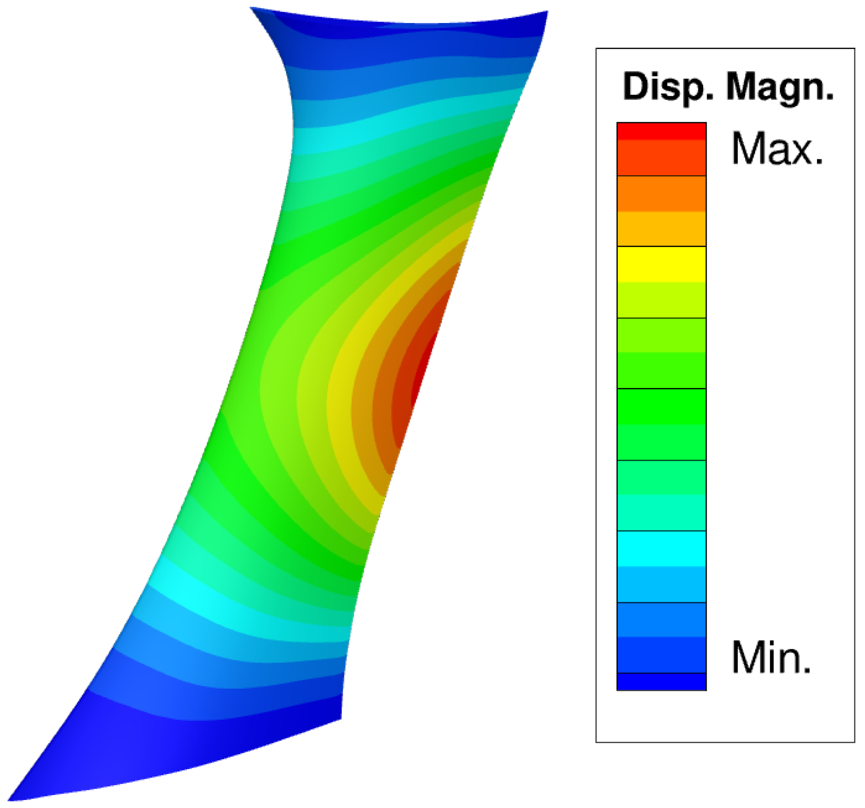
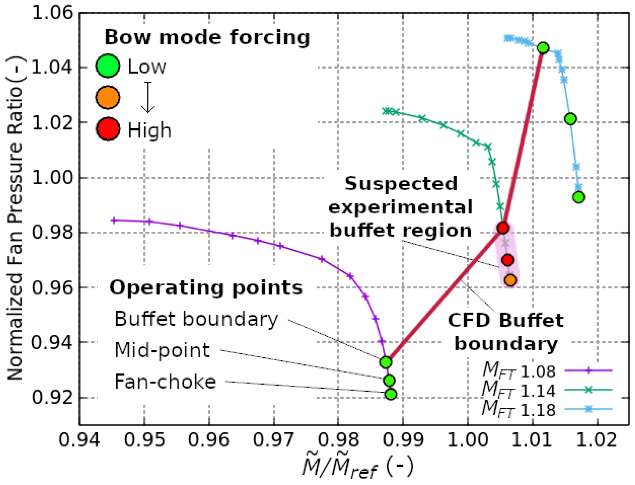
The pursuit of performance and efficiency in aero-engines has led to short, compressed engine architectures, with outlet guide vanes (OGVs) placed closer to the fan and downstream obstructions within the low-pressure system. This has necessitated OGVs being arranged in non-axisymmetric assemblies with individually staggered and cambered blades. Under certain off-design conditions, the aerodynamic instability, known as OGV buffet, can occur on individual blades. This results in buffeting: the structural response to the aerodynamic excitations [1]. This work was originally presented in the conference proceedings of the 14th European Conference on Turbomachinery Fluid dynamics and Thermodynamics [2]. Buffeting is suspected to be the cause of high levels of asynchronous (non-integer multiples of rotational frequency) vibrations detected in off-design tests of a large civil turbofan. The vibration occurred in the first bow mode and high amplitudes were limited to a single vane. The modal displacements in Figure 1 show that the bow mode is most susceptible to excitation at midspan, toward the trailing edge. The vibrations occurred at a high mass flow condition, where the fan was running at a fan-tip Mach number () of = 1.14, which we will refer to as the “datum engine speed”. The simulated fan constant speed characteristic of the datum engine speed is show in green in Figure 2, with the experimental buffeting region highlighted in pink. The vibrations had a reduced frequency of approximately 0.34. The reduced frequency (k) was calculated in line with Equation (1) using angular frequency (), OGV semi-chord (b) and mass-averaged inlet velocity (U).
Previous work used unsteady simulations of a single passage OGV to understand the cause of OGV buffeting. ‘Buffeting’ refers to the structural response and is distinct to the term ‘buffet’, which pertains to the responsible aerodynamic excitations due to instabilities [1]. The unsteady pressure fluctuations of buffet cause these dangerous buffeting structural vibrations, which can lead to the destruction of turbomachinery blades [3].
The previous study indicated that the specific instability responsible for the phenomenon in OGVs is transonic buffet [4]. Typically associated with external aerodynamics, transonic buffet is a flow instability characterised by large-scale, periodic shock motion and a fluctuating shock-induced separation, growing in phase as the shock moves forward and shrinking as it retreats [5]. Transonic buffet occurs when a strong shock-wave–boundary-layer interaction (SBLI) causes the boundary layer to thicken and separate [6]. The shock-induced separation increases in size and spreads to the trailing edge and is followed by unstable self-sustaining shock motion [1].
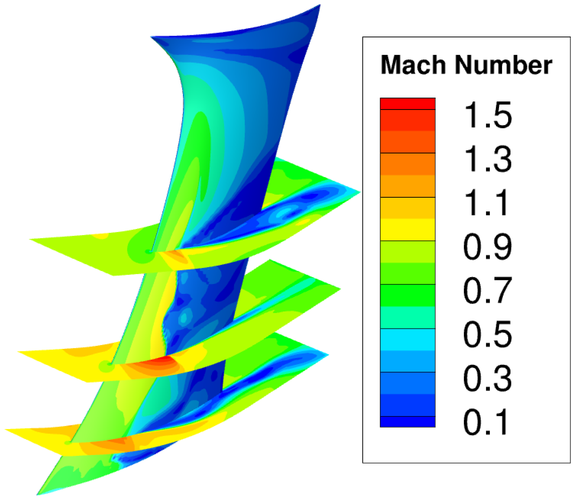
Figure 3 shows an example flow field from a steady solution of a buffeting operating point. The previous study revealed a highly 3D phenomenon, incorporating shock movement with chordwise and radial components, a linked fluctuating separation region and substantial hub separation. Unsteady simulations produced relatively noisy forcing signals, with a dominant frequency very close to that recorded during engine testing. Importantly, the simulations showed that forcing was highest at the experimental engine speed. The simulated operating map and buffet boundary are shown in Figure 2, with buffet occurring on the choke side of the marked buffet boundary. The datum engine speed exhibited the highest amplitude forcing of the bow mode, increasing toward the buffet boundary. Despite being purely aerodynamic and without structural motion, the frequencies of the vibrations were very close to the bow mode frequency.
Similar to the 2D supercritical airfoil experiments of Lee, our 3D simulations found that operating points closest to the buffet boundary provided the highest forcing [7]. In their paper, Lee found that fluctuating normal forces were greatest near the buffet onset and decreased moving further into the buffeting conditions. This paper sets out to achieve a more fundamental understanding of OGV buffeting by moving to a quasi-2D domain and conducting parametric studies of the inlet Mach number and incidence angle.
2. Materials and Methods
The simulations presented here were completed using the steady and unsteady Reynolds-averaged Navier–Stokes (RANS and URANS) solver AU3D. This is the in-house solver of the Imperial Vibration University Technology Centre (VUTC) created and validated for use in turbomachinery settings with aeroelastic capability developed over the last 25 years [8,9,10]. For this study, the RANS and URANS equations were solved using an implicit scheme that is second-order accurate in space and first-order accurate in time. Turbulence modelling was provided by a modified Spalart–Allmaras (SA) one-equation model, and all simulations were run using wall functions to treat the boundary layer. Iovnovich and Raveh show that the SA model provides a good level of accuracy in buffet simulations, with Thiery and Coustols proving it to be suitable for 2D buffet simulations [11,12]. Thiery and Coustols say that, in the case of transonic buffet, the time-scales of the wall-bounded turbulence and shock oscillations are so different that the turbulence can be left to modelling. Aerodynamic modal forcing was computed using unsteady pressure histories from the flow solver, as detailed in [13].
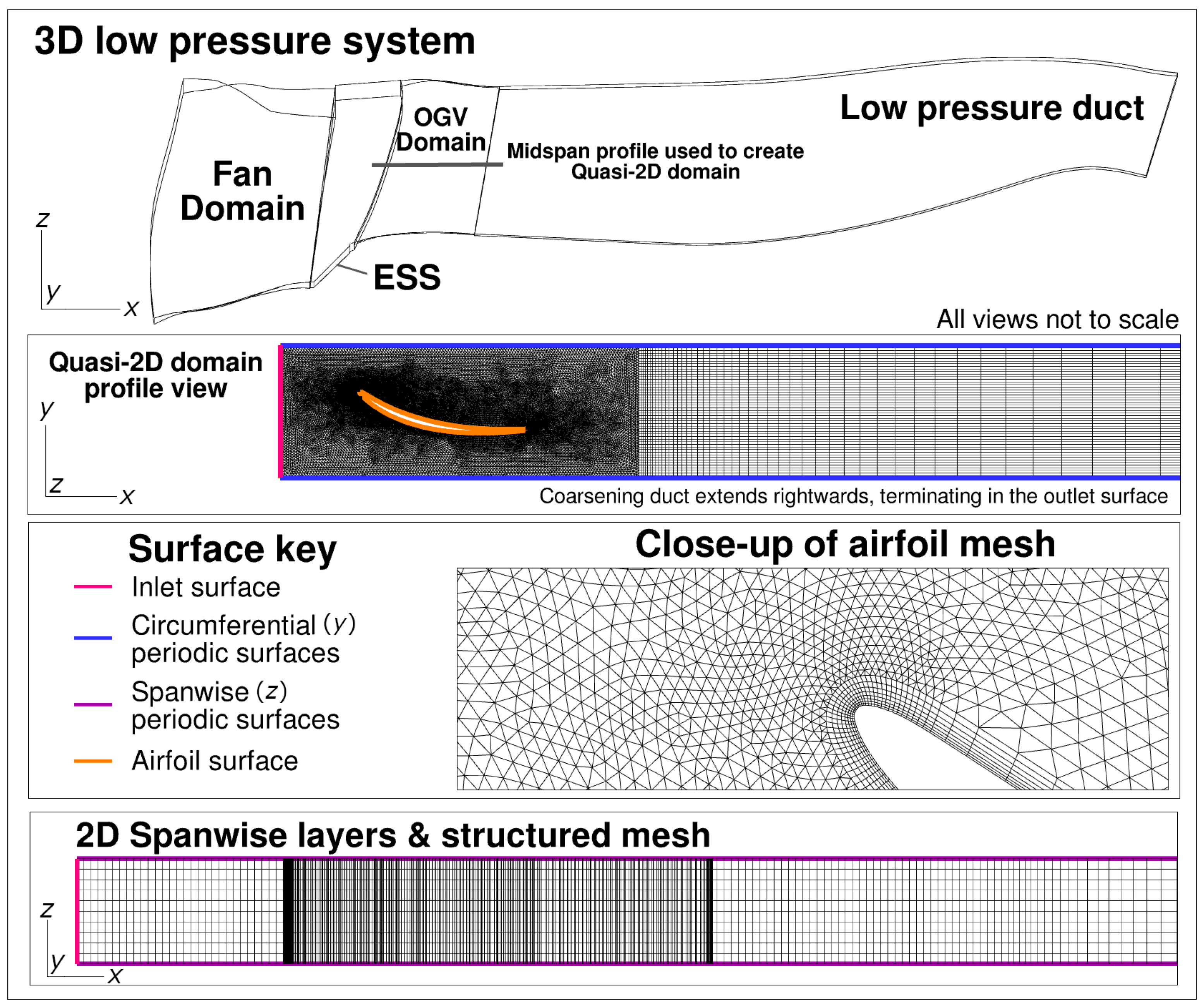
Figure 4 summarises the structure of the 2D domain and its origins in the low pressure system. To construct the 2D domain, the OGV airfoil section at midspan was extracted and meshed in a Cartesian domain using the Altair program HyperMesh. The circumferential width of this slice, presented in the profile view of Figure 4, was based on the OGV pitch at midspan, terminating in y-periodic surfaces. The spanwise extent of the quasi-2D domain is 4% chord resolved with 11 mesh layers connected by structured mesh and terminating in z-periodic boundaries, as shown in Figure 4. The central 2D layer was used to extract all simulation data. The resolution and distribution of nodes in a radial slice were based on previous best practice and produced a Cartesian 2D OGV slice with approximately 20,000 nodes, down from 21,300 used in the layers of the annular 3D domain. The close-up in Figure 4 shows the construction of the unstructured airfoil mesh. Having constructed the OGV domain, a straight coarsening duct was attached approximating the length of the low pressure system. Riemann invariant inlet and outlet boundary conditions and the coarsening duct were used to eliminate numerical reflections. As marked on Figure 4, the OGV inlet surface provides total pressure, total temperature and flow angle boundary conditions, with the outlet surface of the coarsening duct setting a static pressure boundary condition. The periodic set-up meant that all unsteadiness was axisymmetric and not propagating circumferentially, but this was considered satisfactory, as engine testing data indicate that OGV buffet is a local phenomenon. An example simulation with wall functions confirmed that over 80% of node non-dimensional wall distance () values were between 12 and 100, with a mean of 48.
The quasi-2D domain grid was used for all steady RANS and URANS simulations. The datum boundary conditions were derived from area-averaged values for the mixing plane data from the 3D case that provided the highest amplitude forcing. This occurred at the buffet boundary of the datum engine speed. The URANS simulations of the parametric studies were started from a converged steady state RANS solution that was second order accurate in space. The URANS time-step, previously subjected to a convergence study for our 3D work, was carried over and provides a temporal resolution of 390 steps per period of experimental buffeting. Total simulation time was set to provide approximately 25 flow-throughs of the 2D domain and produced consistent results. Time histories were individually trimmed to exclude any initial transients in the following analysis.
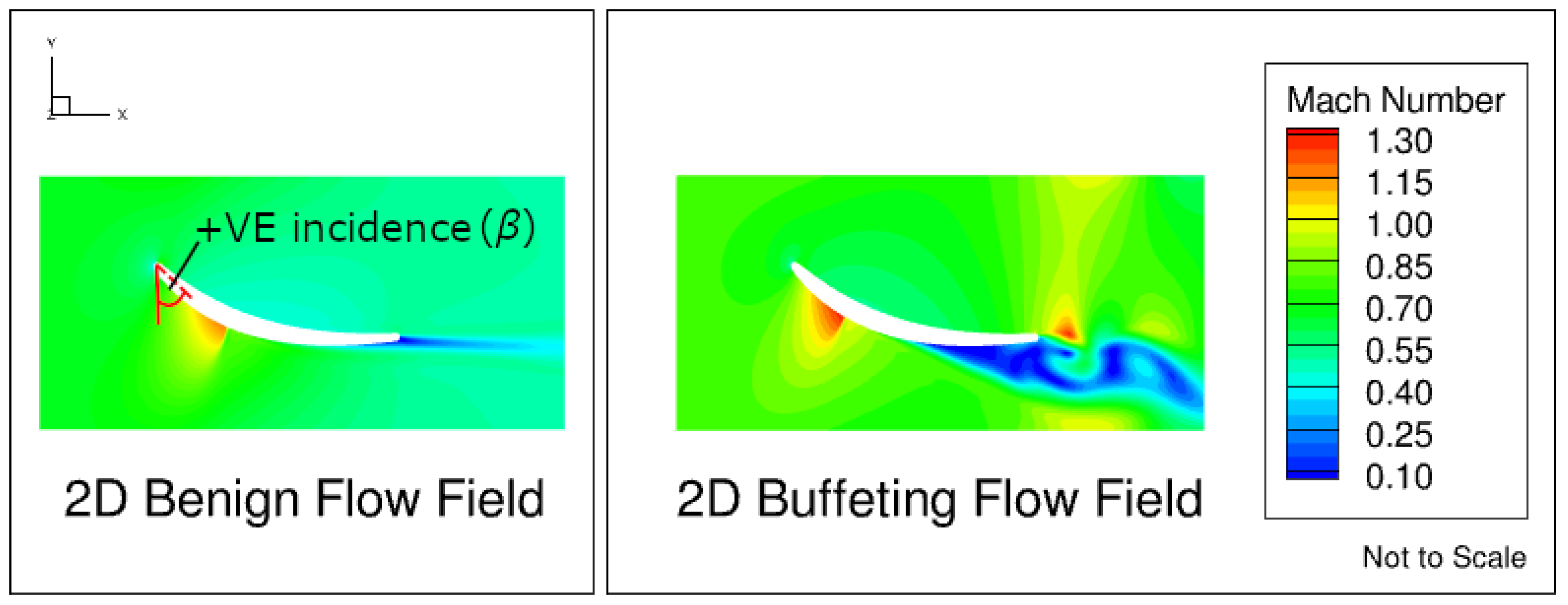
Airfoil incidence and Mach number are known to influence transonic buffet onset and strength [7]. Therefore, the core of this paper is based on two parametric studies, varying inlet Mach number () with airfoil incidence () held constant and vice versa. Incidence was calculated as the difference between the inlet flow angle and metal angle, as shown in Figure 5. Negative incidences are common in this study due to the high axial velocities. and were varied by modifying the specified velocity components of the datum inlet boundary conditions by increasing their resultant magnitude, or their relative magnitude with the resultant held constant, respectively.
For each parametric study, a range of inlet conditions were selected, with increased resolution around the datum values. These operating conditions and the initial 3D-derived datum conditions are summarised in Table 1. Not all of the parametric study operating points produced unsteady forcing, and were therefore deemed to be buffet-free; these are indicated in Table 1 but excluded from the following analysis. Two results have been totally excluded for exhibiting the “carbuncle effect”, a numerical instability responsible for the appearance of a small blister-like structure in high Mach number flows [14].
Figure 5 shows two example full-pitch circumferential cuts of the 2D URANS flow fields of buffeting and non-buffeting (or benign) operating points. The benign flow field has a well-defined shock and minimal TE separation, whereas the buffeting operating point shows many of the characteristics of transonic buffet, including a shock that has shifted in position and a large separation stemming from the base of the shock. The size of this separation also has an effect on the free-stream by decreasing the effective passage area.
3. Results and Discussion
3.1. Forcing Frequency and Amplitude
Time histories of lift forcing were recorded for each operating point and analysed using Welch’s method to produce frequency spectra of the component amplitudes. Monitoring lift was selected to allow us to focus on the 2D causes of the shock motion, which would be complicated by the 3D nature of the first bow mode varying in both span and chordwise directions. Welch’s method operates by splitting the signal into segments and averaging the resulting a with a degree of windowing to reduce the effect of noise. The previous study’s segment size of 4800 time-steps has been retained for reasons of accuracy and comparison.
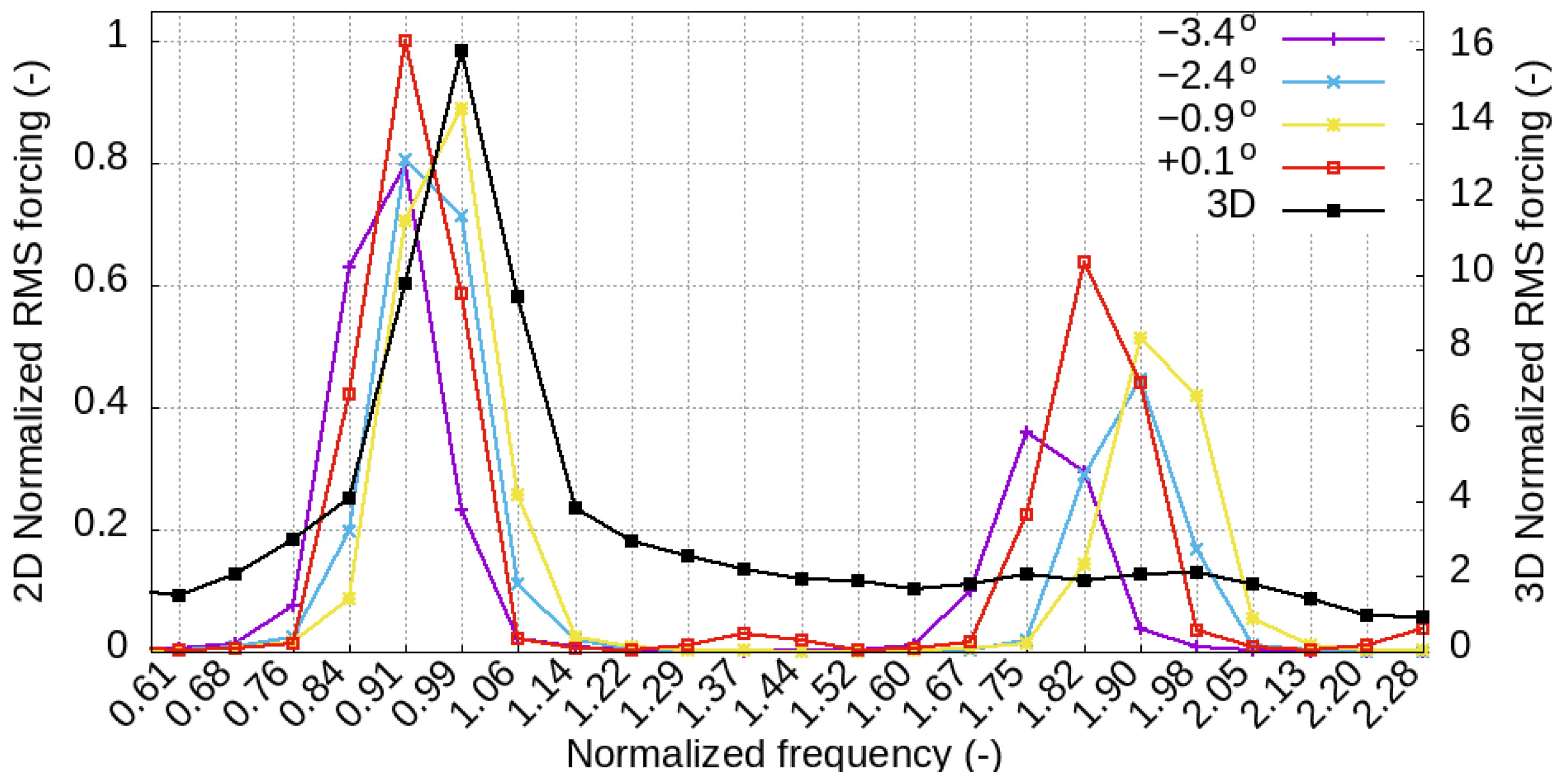
Figure 6 presents resulting selected RMS forcing amplitudes and frequency spectra of the incidence parametric study, normalised by bow mode frequency and maximum amplitude. Only selected 2D results were pictured for reasons of clarity. The spectrum for the original 3D datum case has been included for comparison, scaled to the secondary y-axis. We can see well grouped first harmonics for each buffeting operating point sitting very close to the bow mode frequency and the 3D case. However, the 2D cases all possess clear second harmonics that are proportionally higher in amplitude than the broadband noise of the 3D case.
Within the 2D cases, we can see that the amplitude of the first harmonics broadly increases with but only changes by approximately 20%, with the trend being more pronounced in the second harmonics. There is little difference in frequency between the 2D cases, limited by the normalised frequency resolution of 0.08, dictated by the chosen Welch segment size. The separation is more visible in the second harmonics, showing that the frequency increases with incidence until −2.4, whereupon it remains constant before actually decreasing for +0.1.
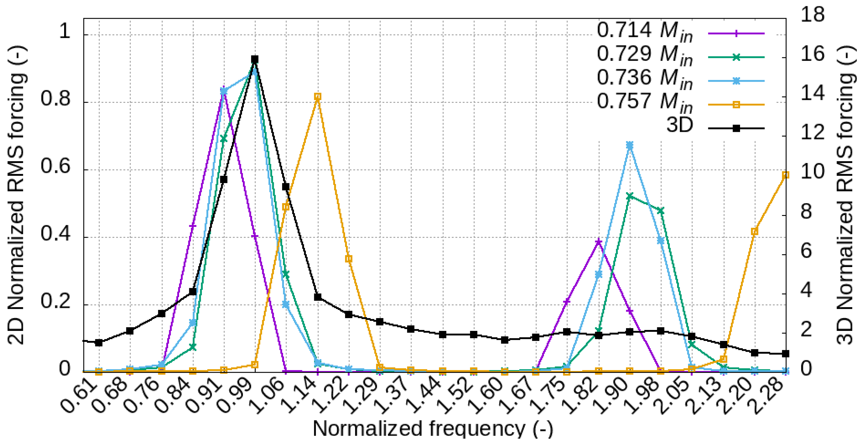
Figure 7 reproduces this analysis for the parametric study and shows a pattern of well-grouped first harmonics slightly increasing in frequency with . Second harmonics also increase in amplitude and frequency, rising well above the proportional 3D broadband noise. However, there is a major outlier in 0.757 that showcases a substantially different first harmonic frequency, which is 14% higher than the bow mode frequency.
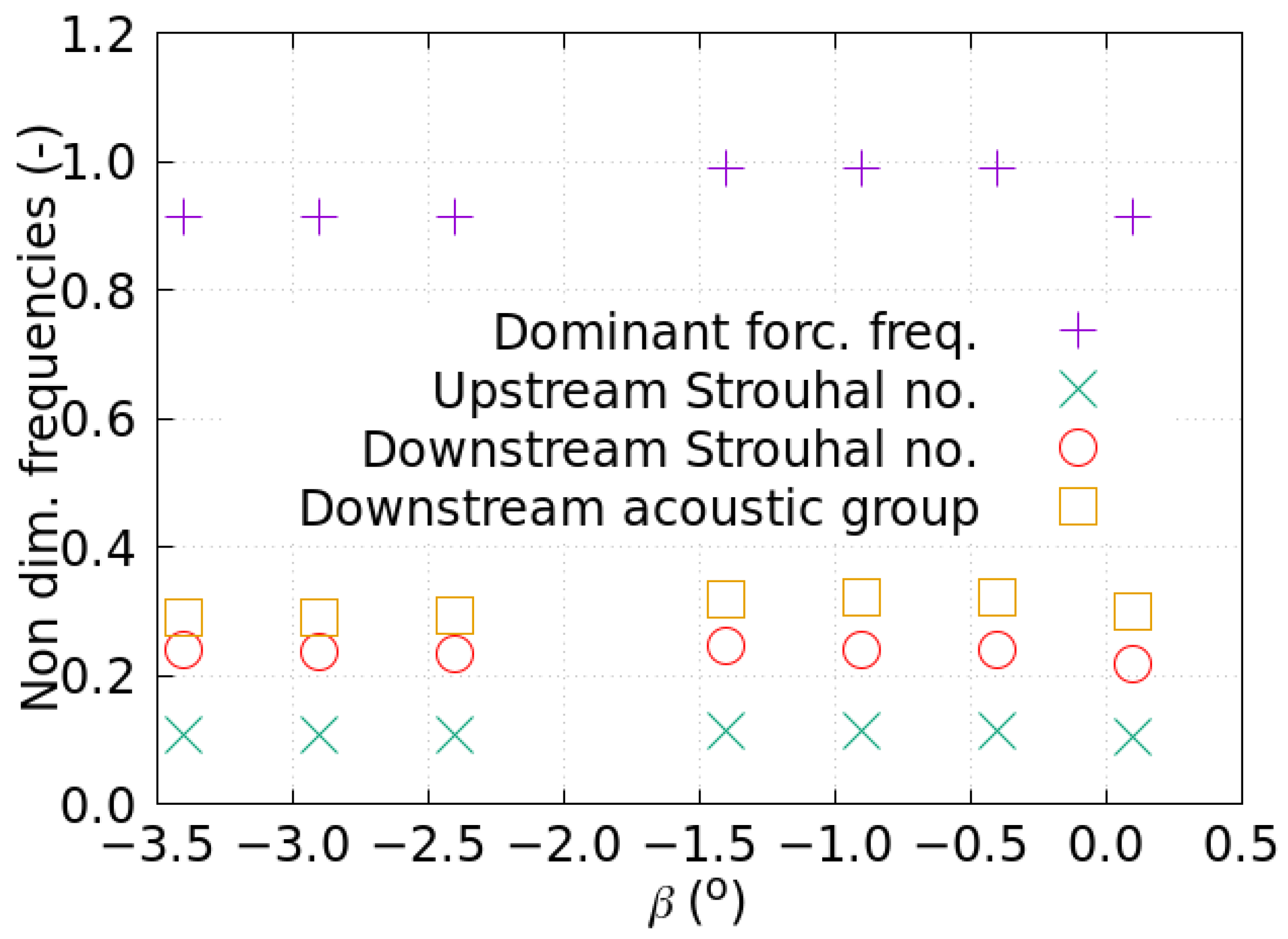
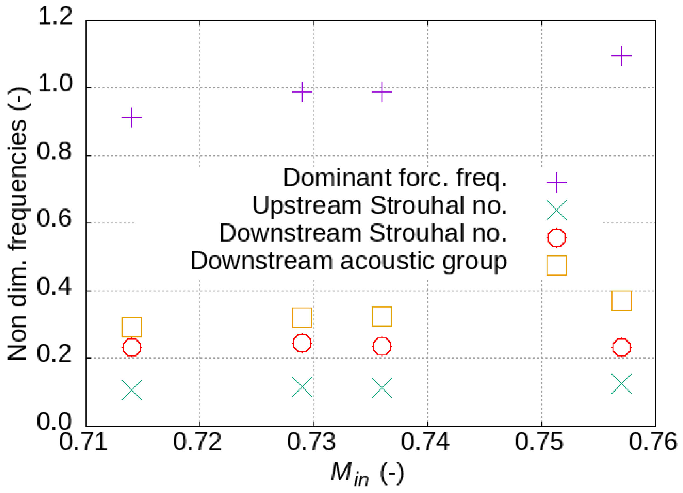
Figure 8 and Figure 9 feature non-dimensional frequencies plotted against the varying incidence and inlet Mach number: the dominant forcing frequency, Strouhal number and an acoustic frequency. The dominant forcing frequency and the acoustic frequency are both normalised by the bow mode frequency. The Strouhal number () can be used to determine whether the aerodynamic unsteadiness occurs at a fixed non-dimensional frequency and is calculated in line with Equation (2), using the dominant forcing frequency (f), OGV chord (C) and two reference velocities: upstream and downstream (U). The upstream velocity was based on the mass-averaged inlet velocity and downstream velocity on the time-averaged profile velocity at 80% chord.
Acoustic feedback mechanisms have been said to be important for self-sustained shock motion and to determine whether this is influencing OGV buffet. Figure 8 and Figure 9 incorporate an acoustic frequency calculated using the downstream velocity to estimate the period of a wave travelling from the shock at 20% span to the TE and returning [15]. From Figure 8, we can see that the dominant forcing frequencies are reasonably flat for increasing , whereas the sweep of in Figure 9 produces gradually increasing dominant frequencies for increasing . This implies that is more important for setting the dominant forcing frequency close to the OGV bow mode, but a wide range of produces the most consistently dangerous frequencies. For both studies, the Strouhal number trends mirror the dominant forcing frequencies but remain relatively consistent, with upstream and downstream Strouhal numbers holding values of approximately 0.1 and 0.24, respectively, albeit with a minor up-tick in the upstream Strouhal number at higher Mach numbers. This consistency indicates a common underlying convective non-dimensional frequency. Figure 8 and Figure 9 show that downstream acoustic frequencies follow similar trends to the dominant forcing frequencies, but at approximately one third of the magnitude, indicating that acoustic feedback may not have a significant bearing on the OGV shock motion.
3.2. Time-Averaged Mach Number
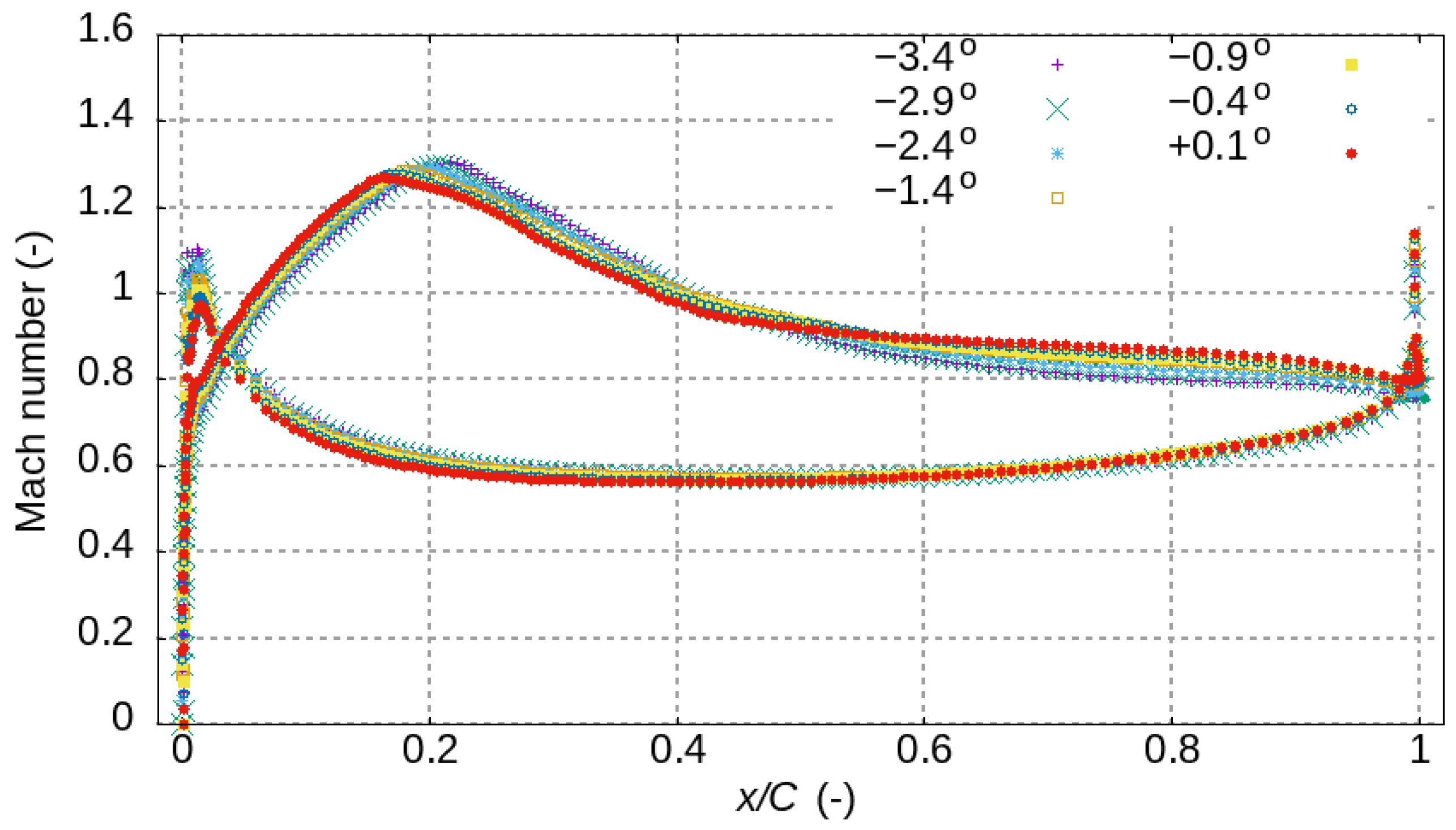
To identify the changes in the flow field responsible for the trends seen above, the profiles of the time-averaged isentropic Mach number were calculated from the time histories of surface pressure for the central mesh layer. Figure 10 shows profiles of the time-averaged Mach number for an increasing incidence. As could be expected for a study where the inlet velocity magnitude was held constant, there is very little change in the overall trend, with each condition possessing a similarly smeared shock, denoting movement. There is a small forward movement of the peak The Mach number location with increasing incidence was accompanied by a small decrease in size. The higher incidences also possess higher Mach numbers toward the trailing edge.
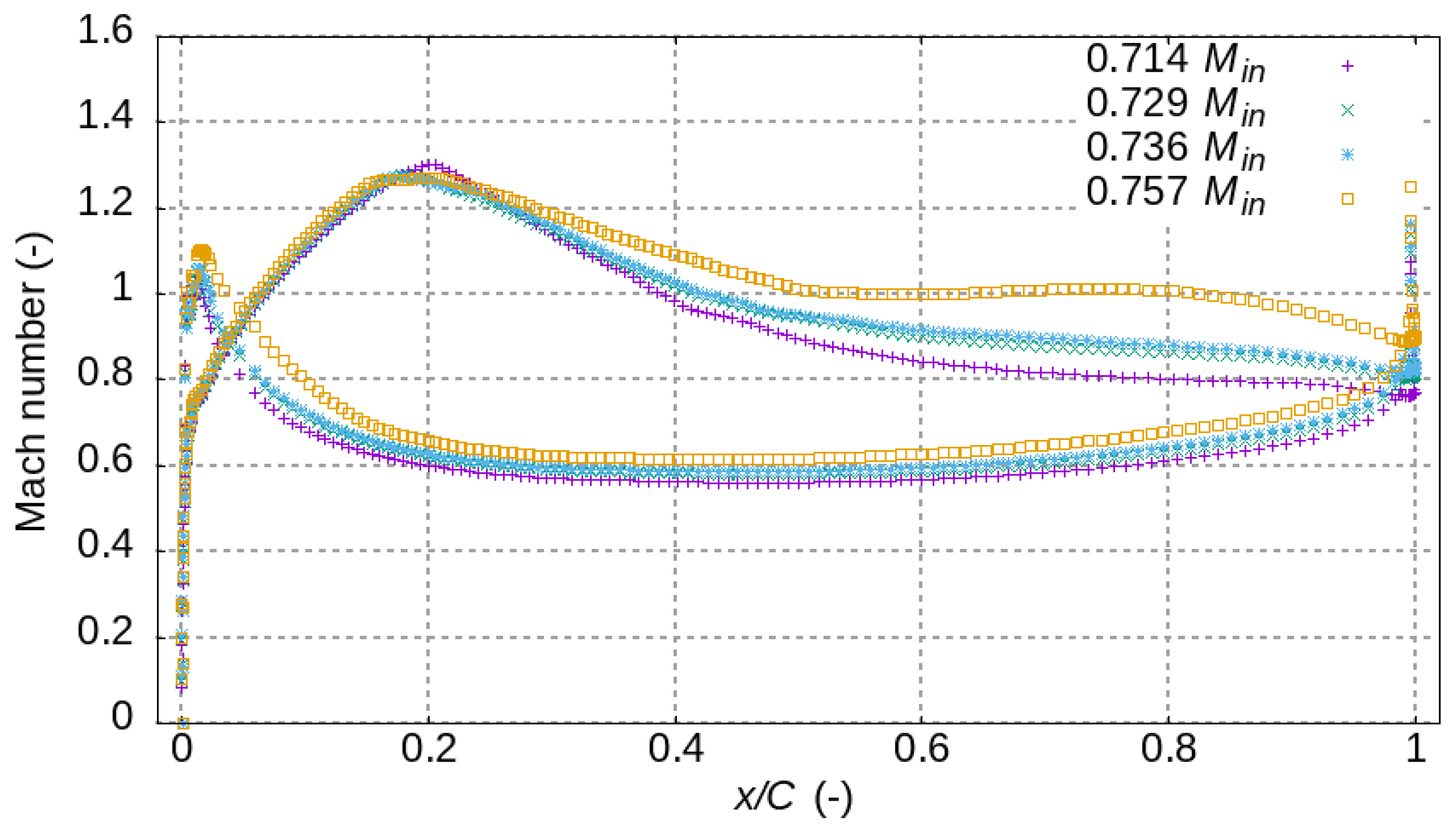
Turning to Figure 11, an increasing gives a similar trend of a forward moving peak, but with a higher sustained Mach number toward the trailing edge for 0.757 . However, an increasing also increases the leading edge pressure surface peak, as opposed to the decrease seen in Figure 10 for an increasing incidence. This is due to negative incidences providing more acceleration around the leading edge.
3.3. Unsteady Pressure Distribution
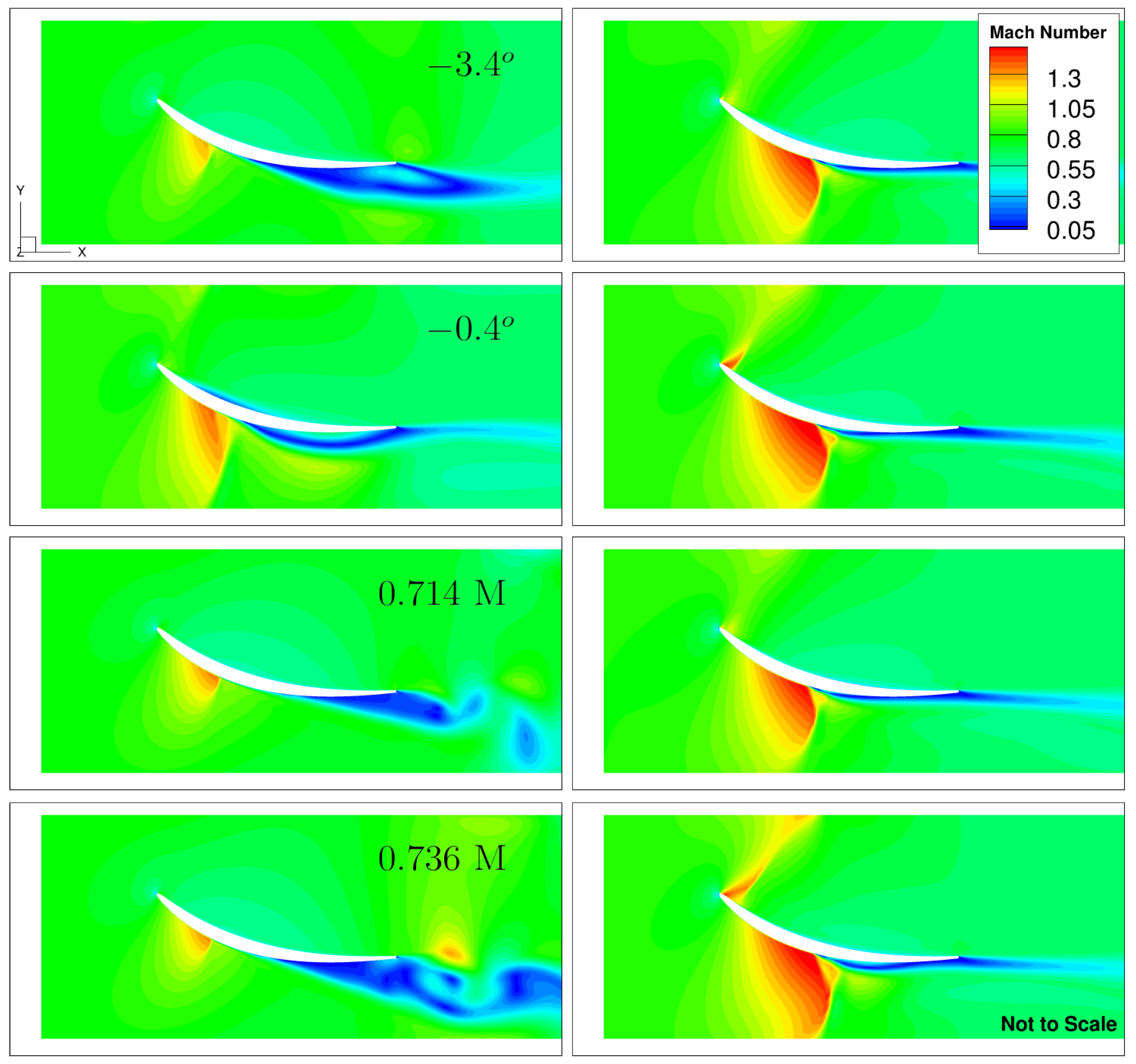
Figure 12 presents full pitch circumferential flow examples for two time steps from four operating points: −3.4, −0.4, 0.714 and 0.736 , showing the progression of buffet in both studies. The snapshots on the left were chosen to show different aspects of flow separation, and those on the right were chosen for their shock strength. All of the separations feature recirculation zones in various stages of creation and ejection. All four cases also experience passage choke when the pressure and suction surface shocks join. However, −0.4 and 0.736 feature shocks were able to move further rearward, have stronger stagnation point shocks and more dramatic shock-wave–boundary-layer interactions on their suction surfaces and went on to exhibit higher unsteady pressure amplitudes. It should be noted that, although only −0.4 shows pressure surface separation, this was at least briefly present in all cases.
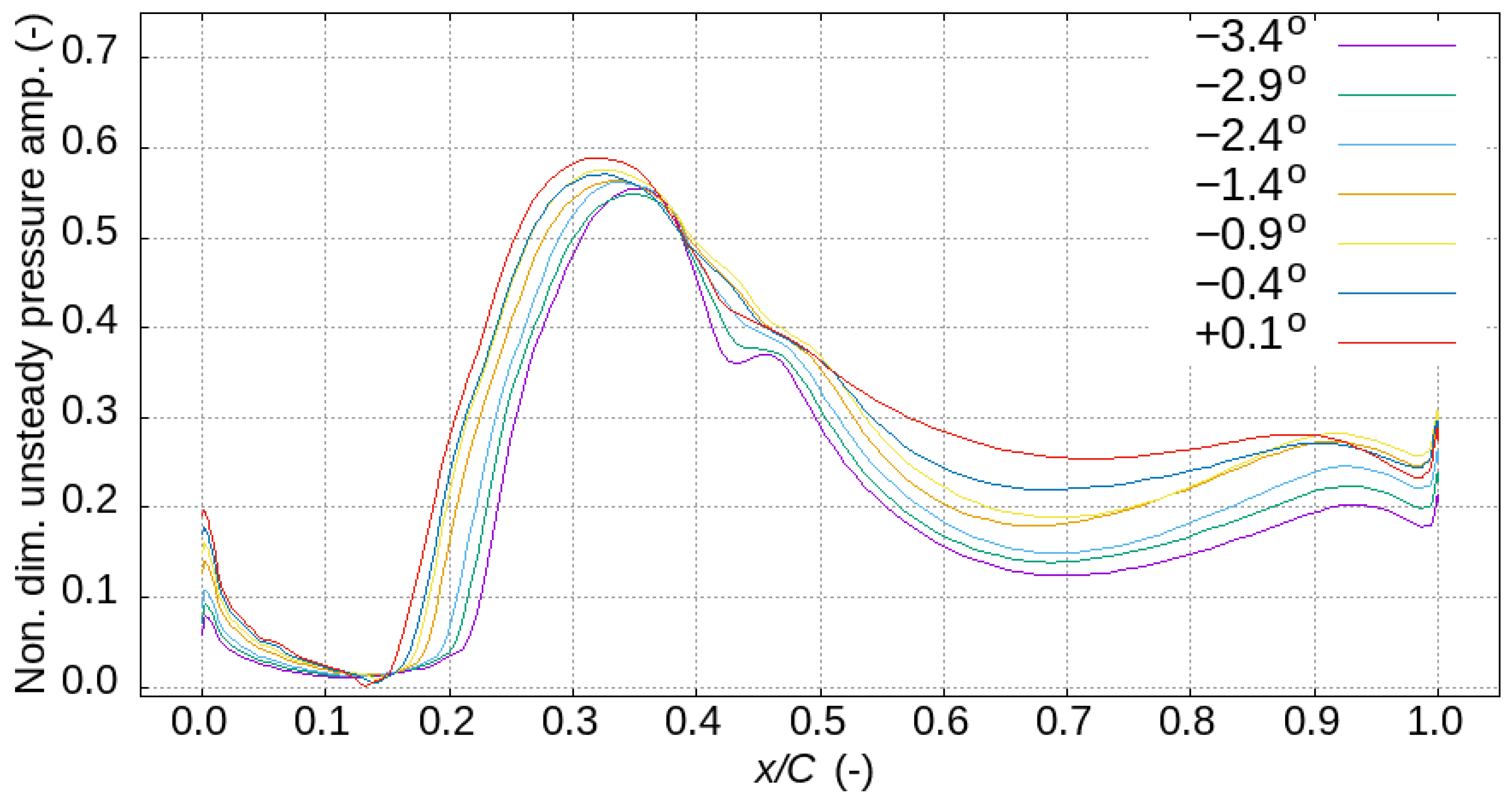
Time histories of surface pressure for the central mesh layer were Fourier-decomposed to calculate unsteady pressure amplitudes in the dominant frequency of each operating point. The plots in Figure 13 and Figure 14 graph unsteady pressure amplitudes, non-dimensionalised by dynamic pressure, against the chordwise location for both the suction and pressure surfaces against . Starting with the baseline of −3.4, we can see a large primary suction peak due to a shock movement at approximately 35% span (15% further aft than peak average Mach number location) and a small secondary peak at 45% span. Lee observed similar secondary peaks due to separation bubbles similar to the recirculation zones identified in Figure 12 [7]. A gradual increase in unsteady pressure amplitudes towards the TE can be attributed to the trailing edge separation [7].
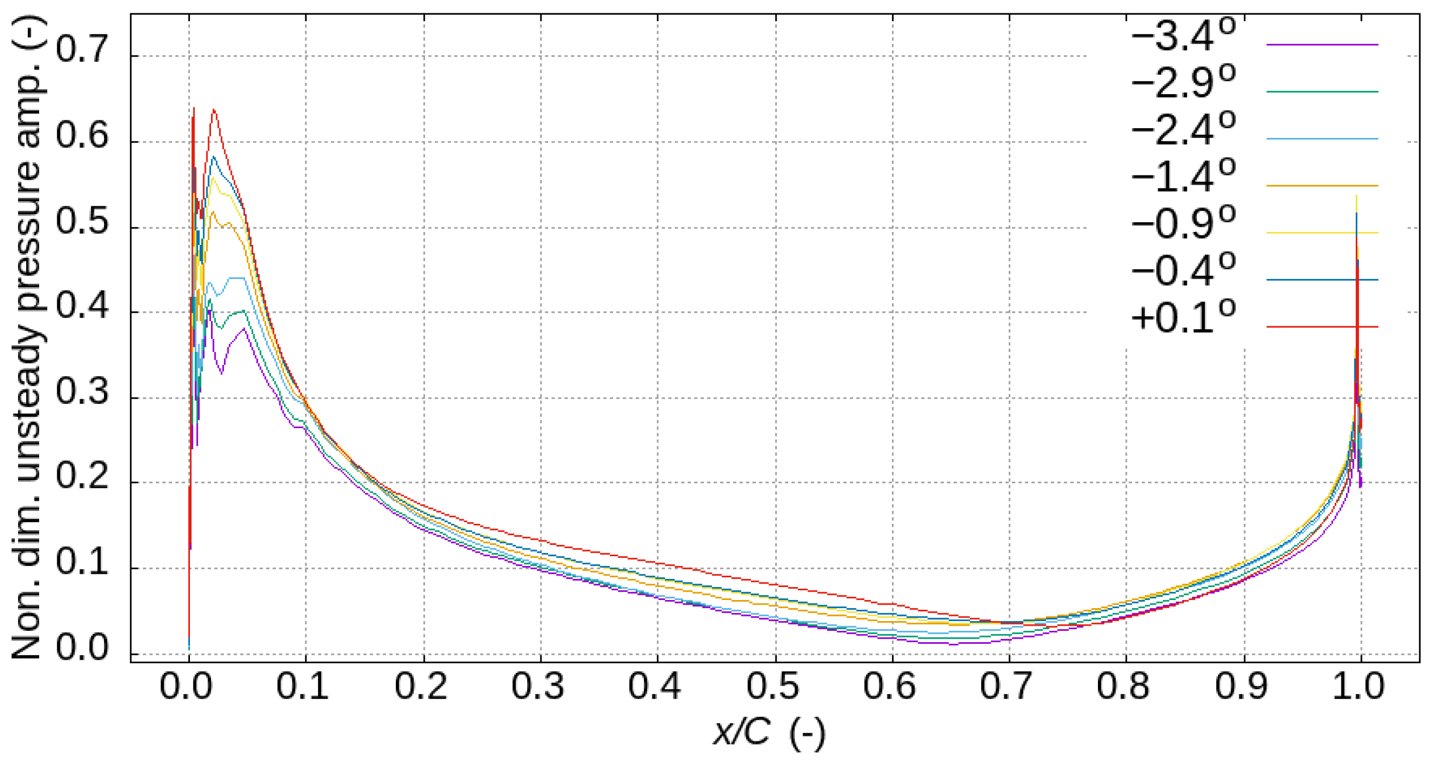
As the incidence increases, the primary peak grows, moves forward and absorbs the secondary peak as the shock displacement grows; this is accompanied by a steady rise in the TE separation fluctuations. An operating point of −0.4 is the only operating point to buck this trend by not providing a distinct increase in the peak and TE separation amplitude. Examining Figure 13, the absorption of a second peak with an increasing incidence seems to be due to the increase in shock strength and movement masking the effect of any recirculation zones. For the pressure surface, as the incidence increases, we see increased amplitudes at the stagnation point and two minor peaks consolidating into one. Analyses of complete time histories reveal this to be caused by the passage-choking pressure surface shock dividing in two as it shrinks. The effect is lessened at higher incidences, as one half becomes substantially stronger and overwhelms the other. This increase in the peak suction and pressure surface unsteadiness with incidence runs counter to the trend of a decreasing peak average Mach number. However, the locations are clearly linked, with the time-averaged suction surface peak Mach number location and peak unsteadiness moving forward with an increasing incidence. The higher unsteady amplitudes towards the trailing edge also correlate with higher time-averaged Mach numbers.
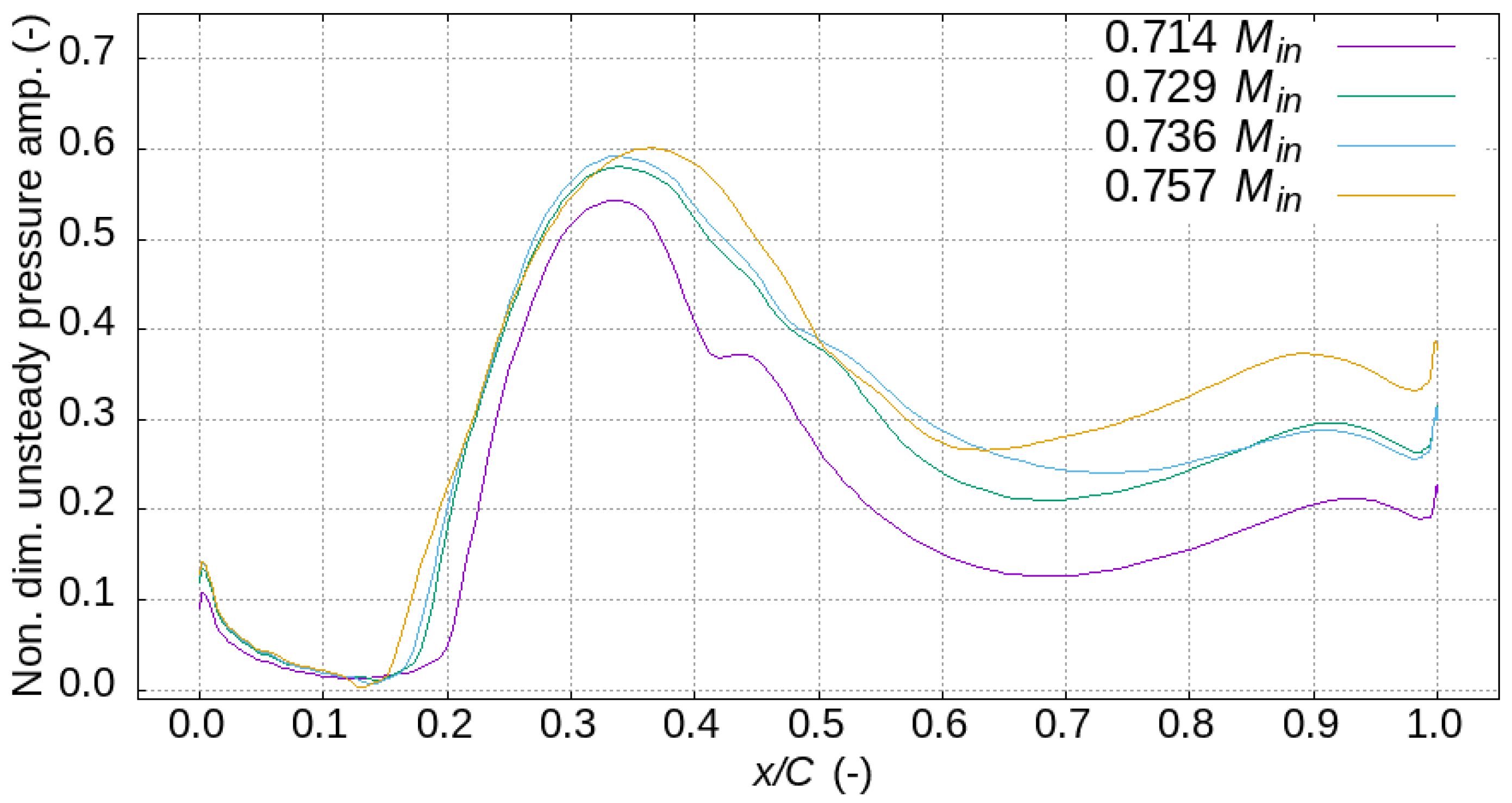
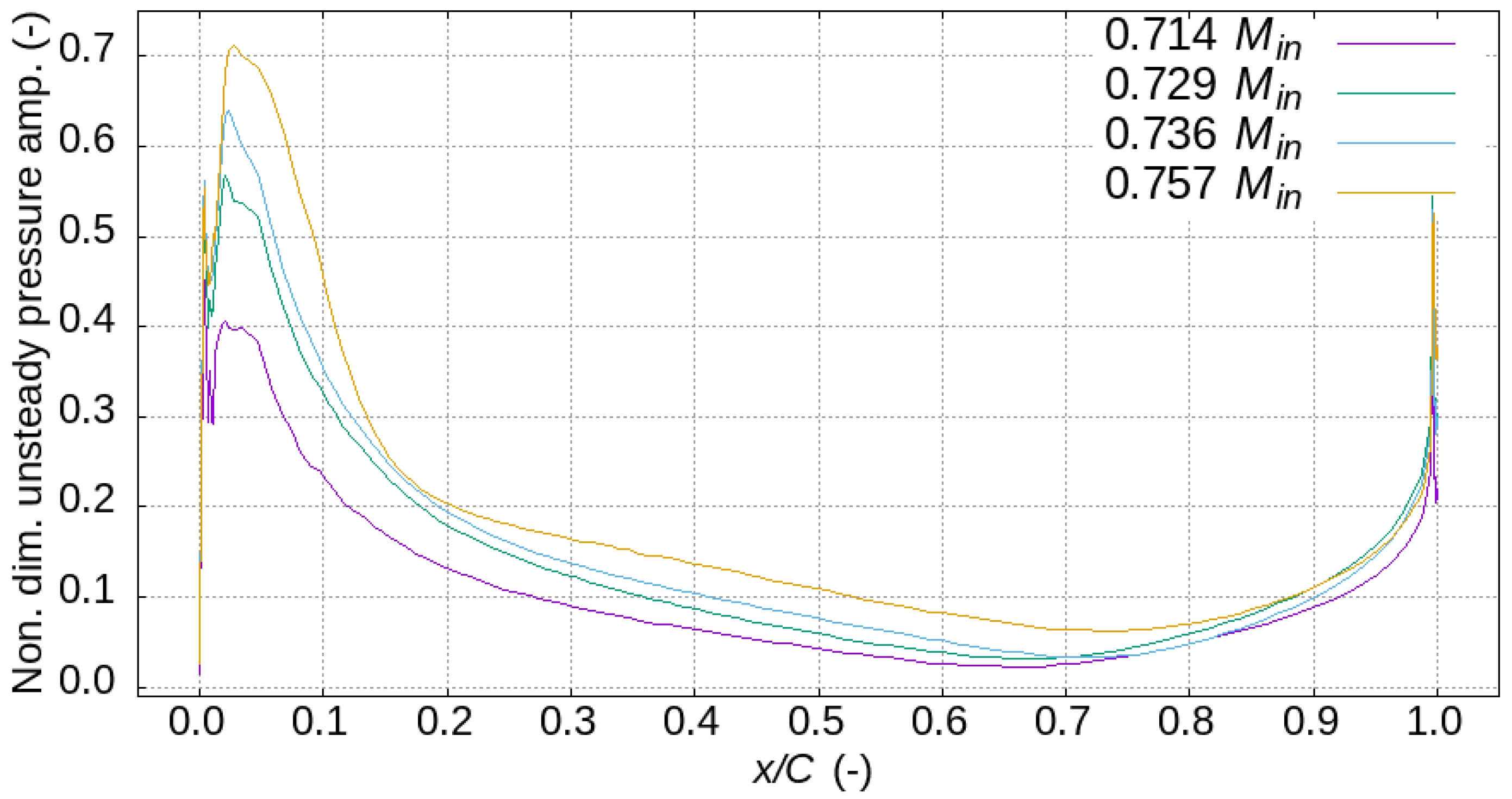
Figure 15 and Figure 16 show similar behaviour for varying , with the only slight difference being that the peak unsteady amplitude location moves aft with increasing , in contrast to the peak average Mach number, which moves forward. In both parametric studies, the broadening of the unsteady amplitude peaks with an increasing inlet Mach number and incidence can be interpreted as an increase in the range of shock motion.
Figure 17 and Figure 18 plot the maximum suction surface unsteady pressure amplitude (normalised by the maximum value across both studies) against varying and . Increasing the inlet Mach number increases the unsteady pressure amplitude at a much greater rate than increasing the incidence within the span of these studies. The trends appear approximately linear in the data ranges available. The fact that we also know that peak average Mach number tends to decrease with the incidence and inlet Mach number infers that these trends of increasing peak unsteadiness are due to increased shock movement and not changes in shock strength. This is corroborated by both incidence and inlet Mach number increases resulting in wider peaks of unsteady pressure on the suction surface, indicating a larger shock movement. Correspondingly, larger changes in the unsteady pressure downstream of the shock towards the trailing edge indicate that the forcing in the bow mode, which has a large displacement toward the trailing edge, will increase with a larger shock movement.
4. Conclusions
In this study, the buffet phenomenon observed on an OGV was reproduced on a quasi two-dimensional geometry. The frequency of the 2D phenomenon was very close to that measured on the 3D geometry. This demonstrates that buffet is not driven by highly three-dimensional flow features but by a quasi-2D shock instability. Parametric studies and varying the incidence and inlet Mach number found that an increasing incidence produced more consistent dominant frequencies nearer the bow mode frequency than an increasing inlet Mach number. The buffeting flow fields were also observed to produce consistent Strouhal numbers across both studies. The studies produced smooth trends of time-averaged Mach numbers, with the maximum average Mach number moving forward and decreasing in magnitude with increasing and . The unsteady pressure amplitude trends were also smooth, increasing in magnitude with both the incidence and inlet Mach number. Secondary peaks, increased TE fluctuations and pressure surface LE peaks were linked to recirculation zones, TE separations and twin LE shocks, respectively.
Author Contributions
Conceptualisation, J.H., B.L. and S.S.; methodology, J.H.; software, J.H., B.L. and S.S.; validation, J.H.; formal analysis, J.H.; investigation, J.H.; resources, S.S. and B.L.; data curation, J.H.; writing—original draft preparation, J.H.; writing—review and editing, J.H. and S.S.; visualisation, J.H.; supervision, S.S. and B.L.; project administration, J.H. and S.S.; funding acquisition, S.S. and B.L. All authors have read and agreed to the published version of the manuscript.
Funding
This research was supported by Rolls-Royce plc and an EPSRC iCASE studentship (iCASE Ref 18000163).
Data Availability Statement
The data in this report are subject to copyright by Rolls-Royce plc and therefore have been presented here in normalised and non-dimensional formats and are unavailable for external distribution, but the corresponding author is very happy to further discuss the implications of the simulations and results.
Acknowledgments
The authors would once again like to thank Rolls-Royce, Imperial College VUTC and Department of Mechanical Engineering for their continued support.
Conflicts of Interest
The results presented here are only possible through the provision of technical resources by Rolls-Royce plc and, as such, have also been passed through them for copyright approval.
Abbreviations
The following abbreviations are used in this manuscript:
| OGV | Outlet guide vane |
| RANS | Reynolds-Averaged Navier-Stokes |
| URANS | Unsteady Reynolds-Averaged Navier-Stokes |
| LE | leading edge |
| TE | trailing edge |
References
- Caruana, D.; Mignosi, A.; Robitaillie, C.; Correge, M. Separated Flow and Buffeting Control. Flow Turbul. Combust. 2003, 71, 221–245. [Google Scholar] [CrossRef]
- Harris, J.; Lad, B.; Stapelfeldt, S. Two Dimensional Investigation of the Fundamentals of OGV Buffeting. ETC. 2021. Available online: https://www.euroturbo.eu/publications/proceedings-papers/etc2021-607 (accessed on 13 December 2021).
- Jacquin, L.; Molton, P.; Deck, S.; Maury, B.; Soulevant, D. Experimental Study of Shock Oscillation over a Transonic Supercritical Profile. AIAA J. 2009, 47, 1985–1994. [Google Scholar] [CrossRef]
- Harris, J.R.; Lad, B.; Stapelfeldt, S. Investigating the Causes of Outlet Guide Vane Buffeting. In Proceedings of the ASME Turbo Expo 2020, Virtual, 21–25 September 2020; Volume 84218. [Google Scholar]
- Babinsky, H.; Harvey, J.K. Shock Wave-Boundary-Layer Interactions; Cambridge University Press: Cambridge, UK, 2011; p. 461. [Google Scholar]
- Crouch, J.D.; Garbaruk, A.; Magidov, D.; Travin, A. Origin of transonic buffet on aerofoils. J. Fluid Mech. 2009, 628, 357–369. [Google Scholar] [CrossRef]
- Lee, B.H.K. Transonic buffet on a supercritical aerofoil. Aeronaut. J. (1968) 1990, 94, 143–152. [Google Scholar]
- Vahdati, M.; Sayma, A.I.; Imregun, M. An Integrated Nonlinear Approach for Turbomachinery Forced Response Prediction. Part II: Case Studies. J. Fluids Struct. 2000, 14, 103–125. [Google Scholar] [CrossRef] [Green Version]
- Dodds, J.; Vahdati, M. Rotating Stall Observations in a High Speed Compressor Part 2: Numerical Study; American Society of Mechanical Engineers (ASME): New York, NY, USA, 2014; Volume 2D. [Google Scholar] [CrossRef]
- Stapelfeldt, S.; Vahdati, M. Improving the Flutter Margin of an Unstable Fan Blade. J. Turbomach. 2019, 141, 071006. [Google Scholar] [CrossRef]
- Iovnovich, M.; Raveh, D.E. Reynolds-Averaged Navier-Stokes Study of the Shock-Buffet Instability Mechanism. AIAA J. 2012, 50, 880–890. [Google Scholar] [CrossRef]
- Thiery, M.; Coustols, E. URANS computations of shock-induced oscillations over 2D rigid airfoils: Influence of test section geometry. Flow Turbul. Combust. 2005, 74, 331–354. [Google Scholar] [CrossRef]
- Sayma, A.I.; Vahdati, M.; Imregun, M. An Integrated Nonlinear Approach for Turbomachinery Forced Response Prediction. Part I: Formulation. J. Fluids Struct. 2000, 14, 87–101. [Google Scholar] [CrossRef] [Green Version]
- Garicano-Mena, J.; Lani, A.; Deconinck, H. An energy-dissipative remedy against carbuncle: Application to hypersonic flows around blunt bodies. Comput. Fluids 2016, 133, 43–54. [Google Scholar] [CrossRef]
- Lee, B.H. Self-sustained shock oscillations on airfoils at transonic speeds. Prog. Aerosp. Sci. 2001, 37, 147–196. [Google Scholar] [CrossRef]
Figure 1.
OGV first bow mode.

Figure 2.
Engine operating map with marked OGV buffet boundary with normalised fan pressure ratio plotted against normalised mass flow rate calculated using non-dimensional mass flow rate () and a reference non-dimensional mass flow rate ().
Figure 2.
Engine operating map with marked OGV buffet boundary with normalised fan pressure ratio plotted against normalised mass flow rate calculated using non-dimensional mass flow rate () and a reference non-dimensional mass flow rate ().

Figure 3.
OGV buffeting Reynolds-averaged Navier–Stokes (RANS) simulation flow field.

Figure 4.
3D OGV within low pressure system and translation to quasi-2D domain.

Figure 5.
Two-dimensional OGV full pitch flow field examples and incidence sign convention.

Figure 6.
Parametric study forcing frequency spectra and amplitudes, varying with constant .

Figure 7.
Parametric study forcing frequency spectra and amplitudes, varying with constant .

Figure 8.
Parametric sweep of , comparing dominant forcing frequency, acoustic frequency and at different locations.
Figure 8.
Parametric sweep of , comparing dominant forcing frequency, acoustic frequency and at different locations.

Figure 9.
Parametric sweep of , comparing dominant forcing frequency, acoustic frequency and at different locations.
Figure 9.
Parametric sweep of , comparing dominant forcing frequency, acoustic frequency and at different locations.

Figure 10.
Midspan time-averaged isentropic Mach number profiles for varying at buffeting operating points.
Figure 10.
Midspan time-averaged isentropic Mach number profiles for varying at buffeting operating points.

Figure 11.
Midspan time-averaged isentropic Mach number profiles for varying at buffeting operating points.
Figure 11.
Midspan time-averaged isentropic Mach number profiles for varying at buffeting operating points.

Figure 12.
Instantaneous full-pitch midspan unsteady flow fields of interest.

Figure 13.
Profiles of Fourier-decomposed unsteady pressure amplitudes on the OGV suction surface for varying .
Figure 13.
Profiles of Fourier-decomposed unsteady pressure amplitudes on the OGV suction surface for varying .

Figure 14.
Profiles of Fourier decomposed unsteady pressure amplitudes on the OGV pressure surface for varying .
Figure 14.
Profiles of Fourier decomposed unsteady pressure amplitudes on the OGV pressure surface for varying .

Figure 15.
Profiles of Fourier-decomposed unsteady pressure amplitudes on the OGV suction surface for varying .
Figure 15.
Profiles of Fourier-decomposed unsteady pressure amplitudes on the OGV suction surface for varying .

Figure 16.
Profiles of Fourier-decomposed unsteady pressure amplitudes on the OGV pressure surface for varying .
Figure 16.
Profiles of Fourier-decomposed unsteady pressure amplitudes on the OGV pressure surface for varying .

Figure 17.
Comparing effect of varying on maximum Fourier-decomposed unsteady pressure amplitudes.

Figure 18.
Comparing effect of varying on maximum Fourier-decomposed unsteady pressure amplitudes.


Table 1.
Parametric study simulation tranche summary.
| Incidence | OGV Buffet | Incidence | Buffet | ||
|---|---|---|---|---|---|
| Datum −1.9 | 0.721 | No | Datum 0.721 | −1.9 | No |
| −6.9 | 0.721 | No | 0.577 | −1.9 | No |
| −4.9 | 0.721 | No | 0.649 | −1.9 | No |
| −3.4 | 0.721 | Yes | 0.667 | −1.9 | No |
| −2.9 | 0.721 | Yes | 0.682 | −1.9 | No |
| −2.4 | 0.721 | Yes | 0.707 | −1.9 | No |
| −1.4 | 0.721 | Yes | 0.714 | −1.9 | Yes |
| −0.9 | 0.721 | Yes | 0.729 | −1.9 | Yes |
| −0.4 | 0.721 | Yes | 0.736 | −1.9 | Yes |
| +0.1 | 0.721 | Yes | 0.757 | −1.9 | Yes |
Publisher’s Note: MDPI stays neutral with regard to jurisdictional claims in published maps and institutional affiliations. |
© 2022 by Rolls-Royce plc. Licensee MDPI, Basel, Switzerland. This article is an open access article distributed under the terms and conditions of the Creative Commons Attribution (CC BY-NC-ND) license (https://creativecommons.org/licenses/by-nc-nd/4.0/).
Share and Cite
MDPI and ACS Style
Harris, J.; Lad, B.; Stapelfeldt, S. Two-Dimensional Investigation of the Fundamentals of OGV Buffeting. Int. J. Turbomach. Propuls. Power 2022, 7, 13. https://0-doi-org.brum.beds.ac.uk/10.3390/ijtpp7020013
AMA Style
Harris J, Lad B, Stapelfeldt S. Two-Dimensional Investigation of the Fundamentals of OGV Buffeting. International Journal of Turbomachinery, Propulsion and Power. 2022; 7(2):13. https://0-doi-org.brum.beds.ac.uk/10.3390/ijtpp7020013
Chicago/Turabian StyleHarris, Jonah, Bharat Lad, and Sina Stapelfeldt. 2022. "Two-Dimensional Investigation of the Fundamentals of OGV Buffeting" International Journal of Turbomachinery, Propulsion and Power 7, no. 2: 13. https://0-doi-org.brum.beds.ac.uk/10.3390/ijtpp7020013