
From data Processing to Knowledge Processing: Working with Operational Schemas by Autopoietic Machines


1
Department of Mathematics, University of California, 520 Portola Plaza, Los Angeles, CA 90095, USA
2
Ageno School of Business, Golden Gate University, San Francisco, CA 94105, USA
*
Author to whom correspondence should be addressed.
Big Data Cogn. Comput. 2021, 5(1), 13; https://0-doi-org.brum.beds.ac.uk/10.3390/bdcc5010013
Submission received: 7 January 2021
/
Revised: 26 February 2021
/
Accepted: 2 March 2021
/
Published: 10 March 2021
(This article belongs to the Special Issue Big Data Analytics and Cloud Data Management)
Abstract
:Knowledge processing is an important feature of intelligence in general and artificial intelligence in particular. To develop computing systems working with knowledge, it is necessary to elaborate the means of working with knowledge representations (as opposed to data), because knowledge is an abstract structure. There are different forms of knowledge representations derived from data. One of the basic forms is called a schema, which can belong to one of three classes: operational, descriptive, and representation schemas. The goal of this paper is the development of theoretical and practical tools for processing operational schemas. To achieve this goal, we use schema representations elaborated in the mathematical theory of schemas and use structural machines as a powerful theoretical tool for modeling parallel and concurrent computational processes. We describe the schema of autopoietic machines as physical realizations of structural machines. An autopoietic machine is a technical system capable of regenerating, reproducing, and maintaining itself by production, transformation, and destruction of its components and the networks of processes downstream contained in them. We present the theory and practice of designing and implementing autopoietic machines as information processing structures integrating both symbolic computing and neural networks. Autopoietic machines use knowledge structures containing the behavioral evolution of the system and its interactions with the environment to maintain stability by counteracting fluctuations.
1. Introduction
Data are objects known or assumed as facts, forming the basis of reasoning or calculation. Data also contain factual information (such as the results of measurements or statistics) used as a basis for reasoning, discussion, or calculation. In the digital computing world, data are the carriers of information in the digital form, which can be transmitted or processed. Data can be naturally represented by named sets where the name may be a label, number, idea, text, process, and even a physical object. The named objects may be decomposed into knowledge structures with inter-object and intra-object relationships and associated behaviors, which can cause changes to their state, form, or content. The role of information-processing structures is to discern the relationships and behaviors of various entities composed of data and evolve their state, form, or content accordingly. Information in the strict sense includes a capacity to change structural elements in knowledge systems [1].
Conventional computers process data and provide a way to handle information stored in these data. However, a system cannot be intelligent if it cannot operate with knowledge [2]. The degree of intelligence depends on the ability to operate with knowledge. This is true both for natural and artificial systems. At the same time, intelligent systems work not directly with knowledge but employ knowledge representations of different types, because knowledge per se is an abstract structure [3]. One of the most powerful and flexible forms of knowledge representations is schema.
The first known utilization of the term schema is ascribed to the outstanding philosopher Immanuel Kant, who did this in his philosophical works [4]. As an example, Kant defined the “dog” schema as a mental pattern of the figure of a four-footed animal, without restricting it to any particular instance from experience, or any possible picture that an individual can have [5]. Later, Head and Holmes employed the notion of a schema in neuroscience using body schemas in their studies of brain damage [6]. Bartlett applied the notion of a schema to the exploration of remembering [7]. One more principal approach to utilization of schemas in psychology was instigated by Jean Piaget. He studied cognitive development from the biological perspective describing it in terms of operation with schemas [8].
Informally, a mental schema is both a mental representation (descriptive knowledge) of the world and operational knowledge that determines action in the world.
Schemas are extensively utilized by people and computers for a diversity of purposes. Cognitive schemas are structures used to organize, enhance, and simplify knowledge of the world around us. For instance, behavior of a businessperson or a manager is based on a variety of cognitive schemas that suggest what to do in this or that situation. An important tool in database theory and technology is the notion of the database schema. It gives a general description of a database, is specified during database design, and is not expected to change frequently [9]. The arrival of the Internet and introduction of XML started the development of programming schema languages. There schemas are represented by machine-processable specifications defining the structure and syntax of metadata arrangements in programming languages. Researchers elaborated various XML schema languages [10,11]. XML schemas, in particular, serve as tools for describing the structure, content, and semantics of XML metadata. Specific schemas were elaborated for energy simulation data representation [12]. A particular concept of a schema has been quite common in programming, where it was formalized and widely utilized in theoretical and practical areas [13,14,15,16]. Dataflow schemas have been used for studies of parallel computations (cf., for example, [17]). One more kind of schemas, interactive schemas, is extensively used in psychology, theories of learning, and brain theory [18,19,20].
Schemas are studied and used in a variety of areas including neurophysiology, psychology, computer science, Internet technology, databases, logic, and mathematics. The reason for such high-level development and application is the existence of different types of schemas (in brain theory, cognitive psychology, artificial intelligence, programming, networks, computer science, mathematics, databases, etc.). Many knowledge structures, for example, algorithmic skeletons [21,22] or strategies, are special cases of operational schemas. To better understand human intellectual and practical activity (thinking, decision-making, and learning) and to build artificial intelligence, we have to be able to work with a variety of schema types. Such opportunities are provided by the mathematical schema theory developed by one of the authors [23,24,25], elements of which are presented in Section 2 of this paper.
There are three classes of schemas: operational, descriptive, and representation schemas. Here we consider only operational schemas. Other types of schemas are studied elsewhere. Schemas in general and operational schemas, in particular, are related to multigraphs. That is, the structure of an operational schema is an oriented multigraph.
In Section 3, we describe operations aimed at construction, transformation, and adaptation of schemas. Presenting some properties of these operations in the form of theorems, we give only outlines of proofs not to overload the work with an unnecessary formalism. In Section 4, we present a powerful theoretical model for operation with schemas, which is called a structural machine [26,27]. In Section 5, we discuss computing structures for operation with schemas. In Section 6, we present some conclusions.
In our exposition, we give simple examples to help the reader to better understand highly abstract structures studied in this paper, because our goal is the development of flexible theoretical tools for the study and advancement of existing computing and network systems.
2. Schemas and Elements of Their Mathematical Theory
The mathematical theory of schemas unifies the variety of approaches to schemas in different areas. It provides a general mathematical concept of a schema on the level of generality that makes it possible to model by mathematical tools virtually any type of schema.
According to the typology of knowledge [3], there are three basic schema types:
- Operational schemas
- Descriptive or categorical schemas
- Representation schemas
Here we consider only operational schemas, which are simply called schemas for simplicity, and their processing, while the two other types and their processing are studied elsewhere.
Note that database schemas of all three types—conceptual, logical, and physical schemas—are descriptive schemas and are not considered in this paper.
There are three types of schema elements: objects (also called nodes or vertices), ports, and ties (also called links, connections, or edges). They belong to three classes:
- Object/node, port, and connection/edge constants.
- Object/node, port, and connection/edge variables.
- Objects/nodes, ports, and connections with variables.
Ports are devices through which information/data arrive (output ports or outlets) and is transmitted from the schema (input ports or inlets). There are constants, variables, and constants with variables ports. For instance, a constant port P can have the variable defining its capacity.
Operational schemas also contain such objects as automata and/or automata-valued variables as their nodes. For instance, it is possible to consider an object variable T that can take any Turing machine as its value.
There are different links between objects/nodes. For instance, there are one-way links and two-way links. Each constant link has a fixed type, while link variables can take values in sets of links having different types, and some link variables can also take a void value. For instance, let elements A and B in a schema Q are connected only by a link variable L. If in the instantiation R of the schema Q, this variable takes the void value, it means that there are no links between A and B in R.
Definition 2.1.
A port schema B (also called a schema with ports) is the system of three sets, three multisets, and three mappings having the following form:
B = (AB, VNB, PB, VPB, CB, VCB, pIB, cB, pEB)
Here, AB is the set of all objects (e.g., automata) from the schema B; the multiset VNB consists of all object variables (e.g., automaton variables) from B; the set CB is the set of all connections/links between the objects and object variables in the schema B; the multiset VCB consists of all link variables, i.e., variables that take values in the links between the objects and object variables in the schema B; the set PB = PIB ∪ PEB (with PIB∩PEB = ∅) is the set of all ports of the schema B, PIB is the set of all ports (called internal ports) of the automata from AB, and PEB is the set of external ports of B, which are used for interaction of B with different external systems and are divided into the input and output ports; the multiset VPB consists of all port variables from B and is divided into two disjunctive sub-multisets VPBin that consists of all variable inlets from B, and VPBout consists of all outlets from the schema B; pIB: PIB ∪ VPB → AB ∪ VNB is a (variable) total function, called the internal port assignment function, that assigns ports to automata; cB: CB ∪ VCB → ((PIbout ∪ VPBout) × (PIbin ∪ VPBin)) ∪ (P′IBin ∪ V′PBin) ∪ (P′IBout ∪ V′PBout) is a (variable) function, called the port-link adjacency function, that assigns connections to ports, where P′IGin, P″Igout, V′PBin , and V′PBout are disjunctive copies of P′IGin, P″Igout, V′PBin, and V′PBout, correspondingly; and pEB: PEB ∪ VPB → AB ∪ PIB ∪ CB ∪ VNB ∪ VPB ∪ VCB is a (variable) function, called the external port assignment function, that assigns ports to different elements from the schema B.
Operational schemas are intrinsically related to automata, because in a general case, an instantiation of an operational schema is a grid automaton. In some sense, operational schemas are grid automata with variables. Grid automata are studied in [28,29]. However, for the sake of easier understanding, here we provide examples of relations between schemas and automata, not for grid automata, but for simpler and better-known automata, which are particular cases of grid automata.
Example 2.1.
A schema of transducer (information processing device) hardware from [30] describes an arbitrary transducer.
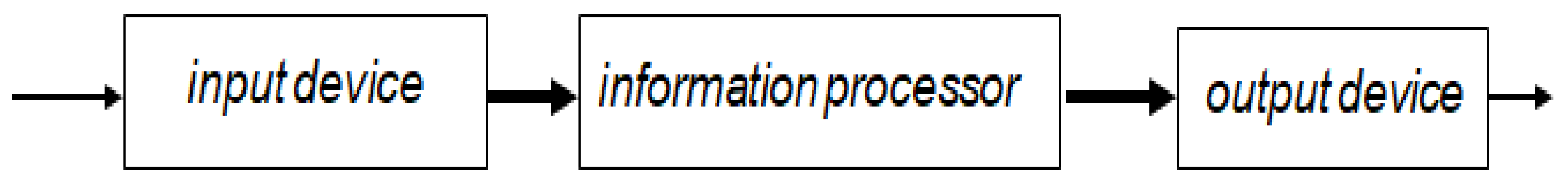
In a general case, the information processing device hardware consists of three main components: an input device, information processor, and output device. This is described by the following schema:
Tr = (VNTr, PTr, VPTr, CTr, VCTr, pITr, cTr, pETr)
VNTr = {ID, IP, OD}, where ID is a variable that takes input devices as values, IP is a variable that takes information processors as values, and OD is a variable that takes output devices as values.
PTr consists of ports from the three device variables, each of which has one input port and one output port.
VPTr consists of port variables attached to the three device variables.
CB is the set of all connections/links between ID, IP, and OD.
VCTr is the set of all connection/link variables, which connect ID, IP, and OD.
cTr is the adjacency function.
An informal visual representation of this schema Tr is given in Figure 1.
Here the variable ID (input device) can take such values as a keyboard, microphone, camera, mouse, or several of these devices together. The variable OD (output device) can take such values as a screen, monitor, printer, plotter, projector, speaker, TV set, headphones, or several of these devices together. The variable IP (information processor) can take such values as a physical system, such as a computer or cell phone, or an abstract automaton such as a Turing machine or register machine.
Example 2.2.
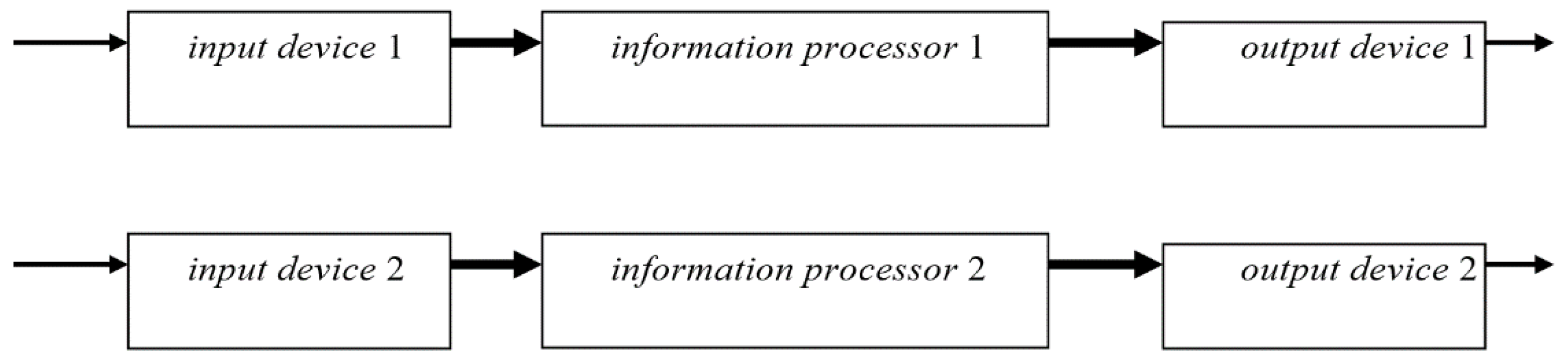
A schema of parallel information processing device hardware describes two independent information processing devices, which can work in the parallel mode.
In a general case, parallel information processing hardware consists of the following main components: two or more input devices, two or more information processors, and two or more output device. The simplest case of such hardware, with two of each device, is described by the following schema:
PTr = (VNPTr, PPTr, VPTr, CPTr, VCPTr, pIPTr, cPTr, pEPTr)
VNPTr = {ID1, IP1, OD1, ID2, IP2, OD2}, where ID1 and ID2 are variables that take input devices as values, IP1 and IP2 are variables that take information processors as values, and OD1 and OD2 are variables that takes output devices as values. These variables are similar to the variables from Example 2.1 and can take similar values.
PPTr consists of ports from the device variables, each of which has one input port and one output port.
VPTr consists of port variables attached to the three device variables.
CPTr is the set of all connections/links between ID1, IP1, OD1, ID2, IP2, and OD2.
VCPTr is the set of all connection/link variables, which connect ID1, IP1, OD1, ID2, IP2, and OD2.
cPTr is the adjacency function.
An informal visual representation of this schema PTr is given in Figure 2.
Definition 2.2.
A basic schema R (also called a schema without ports) has the same organization as the port schema, only without ports. Thus, it consists of two sets, two multisets, and one mapping, i.e., R = (AR, VNR, CR, VCR, cR).
There is a natural correspondence between basic schemas and port schemas. On the one hand, taking a port schema R, it is possible to delete all ports and to change all links between ports by the links between the elements of the schema R, to which these ports belong. On the other hand, taking a basic schema Q, it is possible to attach ports to the elements of the schema Q, to which links are attached in Q.
Example 2.3.
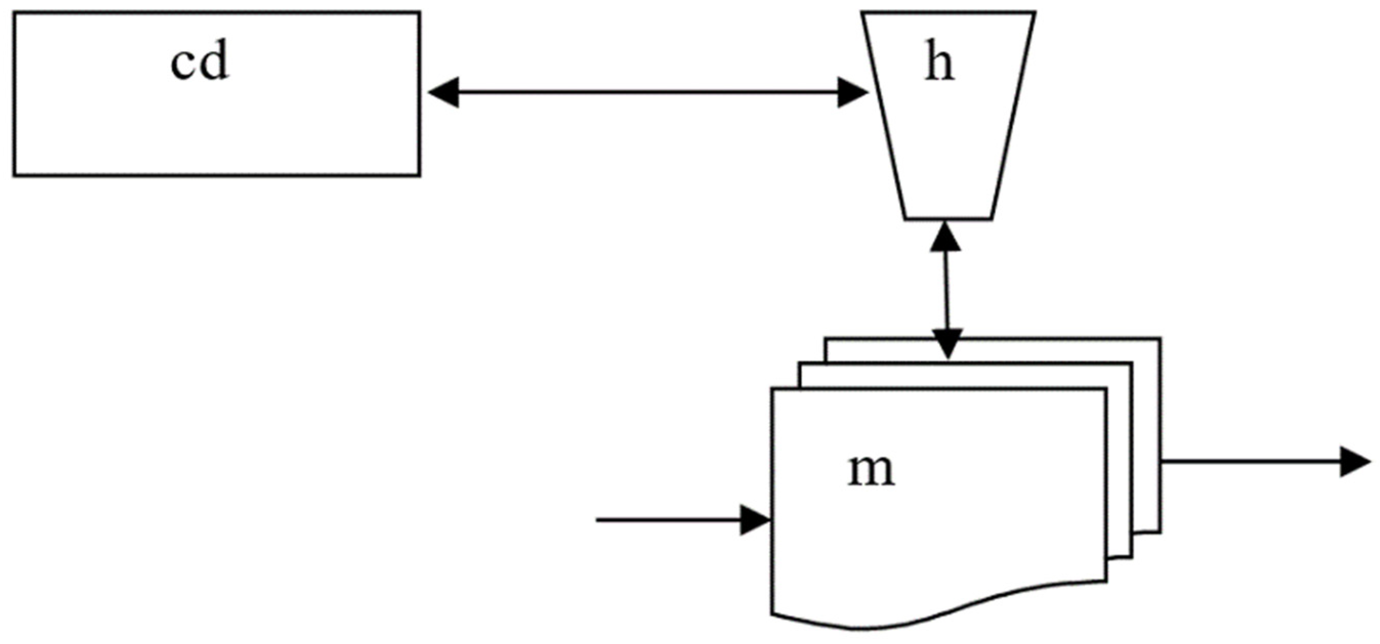
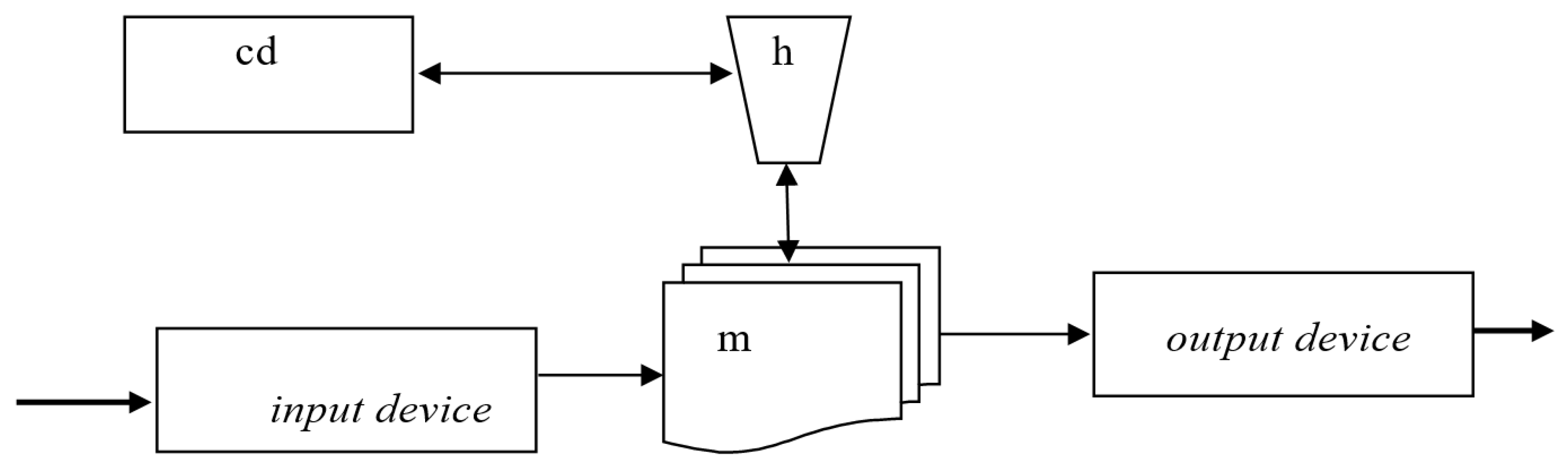
A schema of a Turing machine describes the hardware of an arbitrary Turing machine.
A conventional Turing machine consists of three main components: a control device, information processor, and memory (tape). This is described by the following schema:
Tm = (VNTm, CTm, cTm)
VNTm = {cd, h, m}, where cd is a variable that takes values in accepting finite automata, h is a variable that takes computing finite automata as values, and m is a variable that takes different types of tapes, e.g., one-dimensional, two-dimensional, or n-dimensional tapes, as values.
CTm is the set of all connections/links between cd, h, and m. That is, cd is connected to h, while h is connected to one cell in m.
cTm is the adjacency function between elements/variables and links.
An informal visual representation of this schema Tm is given in Figure 3.
Example 2.4.
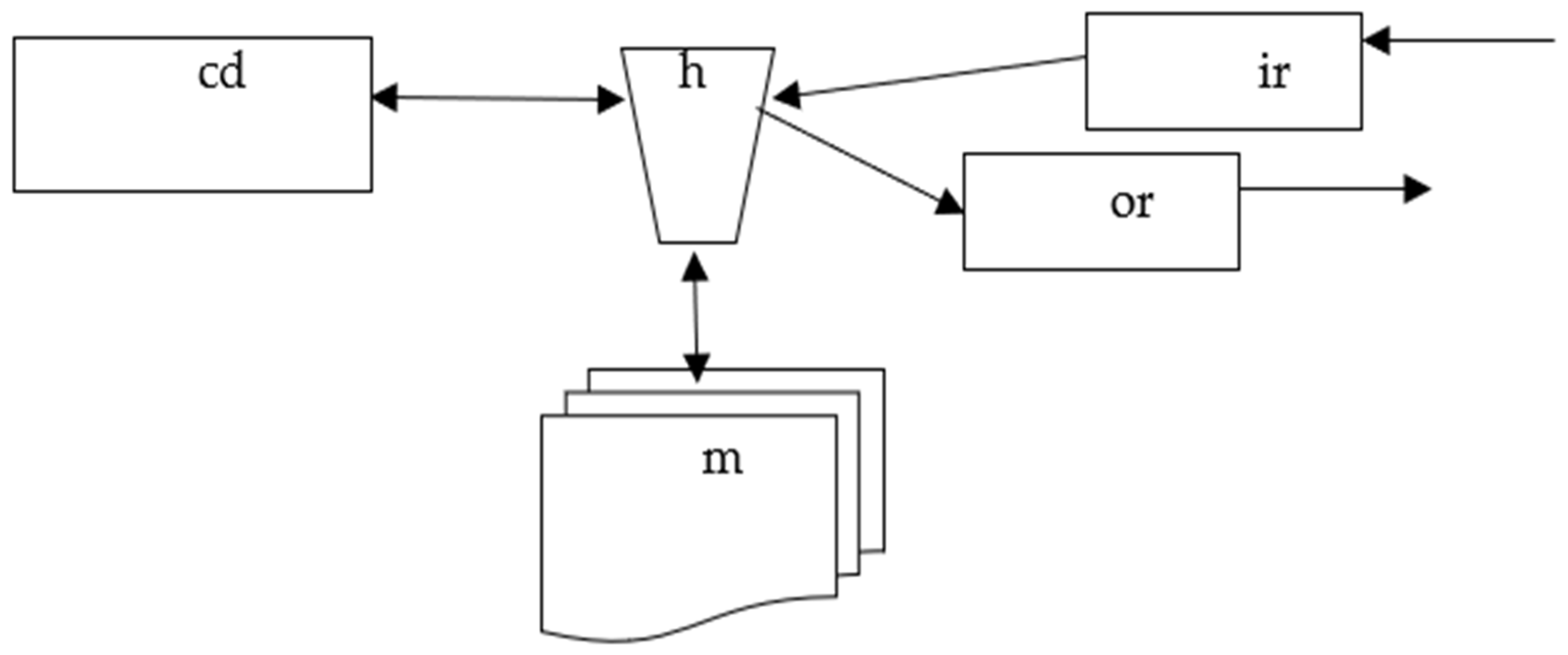
A schema of a simple inductive Turing machine describes the hardware of an arbitrary simple inductive Turing machine [30].
A simple inductive Turing machine consists of five main components: a control device, information processor, input register, output register, and working memory. This is described by the following schema:
ITm = (VNITm, CITm, cITm)
VNTr = {ir, or, cd, h, m}, where cd is a variable that takes values in accepting finite automata, h is a variable that takes computing finite automata as values, ir denotes the input register, or denotes the output register, and m is a variable that takes different types of tapes, e.g., one-dimensional, two-dimensional, or n-dimensional tapes, as values.
CITm is the set of all connections/links between cd, h, and m. That is, the element cd is connected to the element h, while h is connected to one cell in m.
cITm is the adjacency function between elements/variables and links.
Note that in the Turing machine schema and the simple Turing machine schema, the memory is not changing in the process of computation. However, in the higher order inductive Turing machine schema, the memory can be transformed in the process of computation [30]. This difference is not displayed in the schema considered here but can be exhibited in a more detailed schema.
An informal visual representation of this schema ITm is given in Figure 4.
The structure of schema is an oriented multigraph, which is called the grid.
Definition 2.3.
The grid G(P) of a (basic or port) schema P is the generalized oriented multigraph that has exactly the same vertices and edges as P with the adjacency function cG(B) equal to cB.
Example 2.5. ![Bdcc 05 00013 i001]()
The grid of the schema Tm of a Turing machine.

Example 2.6. ![Bdcc 05 00013 i002]()
The grid of the schema ITm of an inductive Turing machine.

3. Operations with Schemas
We discern three types of operations with schemas—large-scale, middle-scale, and local operations.
Types of large-scale operations with schemas:
- Schema processing
- Schema utilization
- Schema transmission
Large-scale operations are formed from middle-scale operations. For schema processing, there are the following types of middle-scale operations with schemas:
- Creation/elaboration of schemas
- Transformation of schemas
- Decomposition/termination of schemas
Utilization of schemas includes the following middle-scale operations (stages):
- Creation of a schema from the existing material
- Formation of a schema instance (instantiation)
- Application of the schema instance
Middle-scale operations are formed from local operations. For schema transformation, there are the following types of local operations with schemas:
- Composition/aggregation of several schemas
- Monotransformation when one schema is changed
- Coordinated transformation of several schemas—polytransformation
Let us consider some of them:
- Outside clutching (also called external composition) con(A, B) of schemas A and B is composed by correct attaching some external ports of the schemas A and B to one another.
An example of outside clutching is sequential composition, which is the most popular operation in computing, where the output port of one computing system is connected to the input port of another computing system. As a result, the output of the first computing system is used as the input of the second computing system.
Example 3.1. ![Bdcc 05 00013 i003]()
Outside clutching (external composition) con(Tr1, Tr2) of the schemas Tr1 and Tr2, each of which is isomorphic to the schema Tr (cf. Example 2.1).

Theorem 1.
If the connection of the external ports remains the same, then the outside clutching (external composition) of schemas is a commutative operation, i.e., con(A, B) = con(B, A) for any schemas A and B.
Proof is done by induction on the number of the new connections and is based on the following properties of schemas. The external ports of the schemas A and B become internal ports in their outside clutching con(A, B). If p and q are internal ports of a schema, then the connection (p, q) is equal to (the same as) the connection (q, p).
- 2.
- Mixed clutching (also called incorporation) inc(A, B) of schemas A and B is composed by correct attaching the external ports of the schema B to the internal ports of the schema A.
An example of mixed clutching is adding an additional chip to a computer or embedded device.
- 3.
- Inside clutching icl(A, B) of schemas A and B is composed by correct attaching the internal ports of schemas A and B.
An example of mixed clutching is adding a feedback link, which goes from the output registers to the input registers.
- 4.
- Substitution:
- Node substitution sub(A, a; B) of a node a in the schema A by the schema B is constructed by eliminating the node a from the schema A and connecting the external links of the node a to the appropriate external ports of the schema B.
- Link substitution sub(A, l; B) of a link l in the schema A by the schema B is constructed by eliminating l from the schema A and connecting the input ports of the schema B to the source of l and the output ports of B to the target of l.
- Component substitution sub(A, C; B) of a component C in the schema A by the schema B is constructed by connecting external links of the component C to appropriate external ports of the schema B.
Example 3.2.
The node substitution sub(Tr, IP; Tm) of the variable IP in the schema Tr of a transducer by the schema Tm of a Turing machine (cf. Example 2.3).
The schema Tr

An informal visual representation of the result of the substitution sub(Tr, IP; Tm) is given in Figure 5.
Let us consider two schemas A and B. Properties of substitution imply the following result:
Lemma 1.
All elements in the schemas A and B but the element a are not changing in the substitution sub(A, a, B).
In contrast to clutching, substitution is not commutative. At the same time, under definite conditions, substitution is associative.
Theorem 2.
Substitution of different elements in a schema is an associative operation, i.e., if a and b are different elements of a schema A, then sub(sub(A, a, B), b, C) = sub(sub(A, b, C), a, B) for any schemas C and B.
Proof is done by induction on the number of the new connections and is based on the following properties of schemas. When the substitution of the schema C in the schema sub(A, a, B), then only the element b is changed, and this element does not belong to the schema B. When the substitution of the schema B in the schema sub(A, b, C), then only the element a is changed, and this element does not belong to the schema C.
- 5.
- Free composition A*B of schemas A and B is constructed by taking unions of their elements, i.e., AA*B = AA ∪ AB, VN(A*B) = VNA ∪ VNB, PA*B = PA ∪ PB, VP(A*B) = VPA ∪ VPB, CA*B = CA ∪ CB, and VC(A*B) = VCA ∪ VCB.
Example 3.3.
The schema PTr (cf. Example 2.2) is a free composition of the schemas Tr1 and Tr2, each of which is isomorphic to the schema Tr (cf. Example 2.1).
Theorem 3.
Free composition of schemas is a commutative and associative operation.
Proof of commutativity is similar to the proof of Theorem 1 and proof of associativity is similar to the proof of Theorem 2.
4. Structural Machines as Schema Processors
To be able to efficiently process knowledge, a computer or network system must have knowledge-oriented architecture and assembly of operations. The most powerful and at the same time, flexible, model of computing automata is a structural machine [27]. It provides architectural and operational means for operation with schemas.
For simplicity, we consider structural machines of the first order, which work with first-order structures.
Definition 4.1.
A first-order structure is a triad of the following form:
A = (A, r, R)
In this expression, we have the following:
- Set A, which is called the substance of the structure A and consists of elements of the structure A, which are called structure elements of the structure A
- Set R, which is called the arrangement of the structure A and consists of relations between elements from A in the structure A, which have the first order and are called structure relations of the structure A
- The incidence relation r, which connects groups of elements from A with the names of relations from R
Lists, queues, words, texts, graphs, directed graphs, mathematical and chemical formulas, tapes of Turing machines, and Kolmogorov complexes are particular cases of structures of the first order that have only unary and binary relations. Note that labels, names, types, and properties are unary relations.
Definition 4.2.
A structural machine M is an abstract automaton that works with structures of a given type and has three components:
- The unified control device CM regulates the state of the machine M.
- The unified processor PM performs transformation of the processed structures and its actions (operations) depend on the state of the machine M and the state of the processed structures.
- The functional space SpM is the space where operated structures are situated.
The functional space SpM, in turn, consists of three components:
- The input space InM, which contains the input structure.
- The output space OutM, which contains the output structure.
- The processing space PSM, in which the input structure(s) is transformed into the output structure(s).
We assume that all structures—the input structure, the output structure, and the processed structures—have the same type. In particular, the functional, input, output, and processing spaces have definite topologies defined by the systems of neighborhoods [26].
Computation of a structural machine M determines the trajectory of computation, which is a tree in a general case and a sequence when the computation is deterministic and performed by a single processor unit.
There are two forms of functional spaces, SpM and USpM:
- SpM is the set of all structures that can be processed by the structural machine M and is called a categorical functional space.
- USpM is a structure for which all structures that can be processed by the structural machine M are substructures and is called a universal functional space.
There are three basic types of unified control devices:
- It can be one central control device, which controls all processors of the structural machine.
- It can consist of cluster control devices, each of which controls a cluster of processors in the structural machine.
- It can consist of individual control devices, each of which controls a single processor in the structural machine.
There are three basic types of unified processors:
- A localized processor is a single abstract device, which consists of one or several processor units or unit processors functioning as a unified whole.
- A distributed cluster processor consists of unit processors (processor units) from a cluster, which performs definite functions in a structural machine.
- A distributed total processor consists of a system of all unit processors (processor units) from a structural machine.
It is possible to treat a localized processor as a singular unit processor although it can be constructed of several processor units, which are moving together processing information. Examples of distributed cluster processors are systems of processors that perform parallel or pipeline transformations of data in the memory.
Structural machines can process information in different modes [31]. This brings us to three kinds of structural machines:
- Recursive structural machines, in which all processors work in the recursive mode.
- Inductive structural machines, in which all processors work in the inductive mode.
- Combined structural machines, in which some processors work in the recursive mode, while other processors work in the inductive mode.
It is proved that for any Turing machine and thus for any recursive algorithm A, there is an inductive Turing machine M that simulates functioning of A [30]. Similar reasoning gives us the following result:
Theorem 4.
For any recursive or combined structural machine R, there is an inductive structural machine Q that simulates functioning of R.
Properties of inductive Turing machines [30] also imply the following result:
Theorem 5.
Inductive and combined structural machines are essentially more powerful than recursive structural machines.
Architectural and functional features of structural machines provide diverse possibilities to perform operations with schemas. For instance, a singular unit processor can move from one location to another location in a schema, acting upon the operated schema. Another option is parallel or concurrent operation of several unit processors performing the necessary transformations of the operated schema.
5. Computing Structures for Operation with Schemas
Digital information processing systems of the current generation are composed of computing structures that are stored program implementations of the Turing machines. As mentioned in this paper, they are designed to transform one state of the data structure, which is a representation of the arrangement, relationships, and contents of data, to another state based on a specified algorithm. The data structure consists of the knowledge about various data elements and the relationships between them. The behaviors of how events alter the data structures are captured in the algorithm (encoded as a program) and are executed to change the state of the knowledge structure using the CPU. Digital computing structures use programming languages, which operate on a variety of data structures such as characters, integers, floating-point real number values, enumerated types (i.e., a small set of uniquely named values), arrays, records (also called tuples or structs), unions, lists, streams, sets, multisets, stacks, queues, double-ended queues, trees, general graphs, etc. In addition, word processors, such as Word or TeX, work with various geometrical shapes, figures, and pictures.
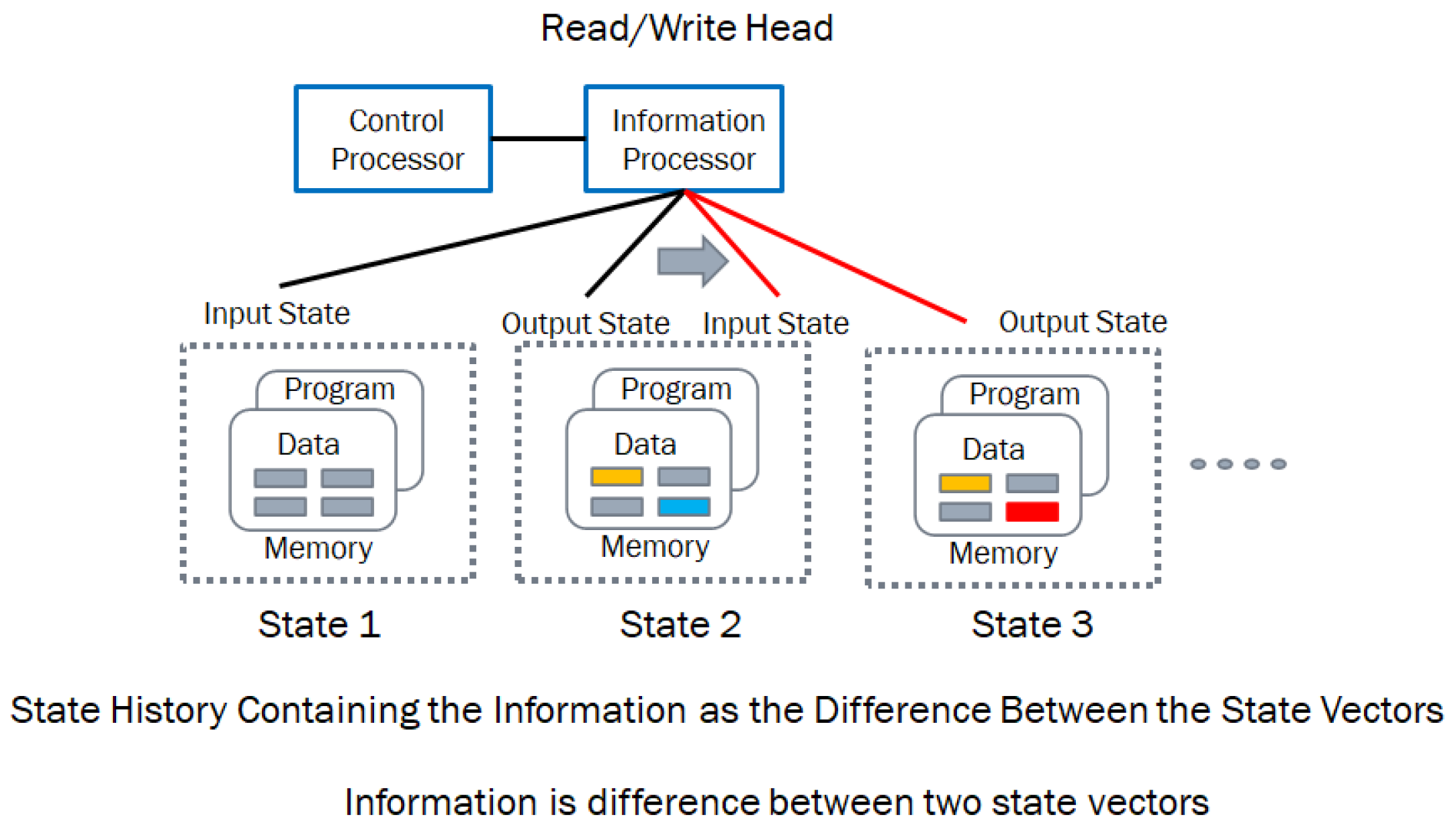
Figure 6 shows the schema and the data structure evolution of a Turing machine stored program control implementation. The schema represents the control processor that executes [30] the infware, the information processor which provides the hardware (CPU and memory) and the software (the algorithms operating on the data structures.) The memory provides both the program and the data for processing.
In essence, information is the change between the data structures from one instant to another, and information processing consists of physical structures that execute the behaviors transforming the data structures from one state to another with a read – compute – write cycle of operations. The digital computing structure requires hardware (the processor and memory) and software (which provides the algorithm and the data structure). In addition, we need the knowledge to configure, monitor, and operate the digital computing structure to execute the algorithm, which is called the infware [30]. The current state of the art requires a third party to execute the infware (an operator or other digital automata), which is given this knowledge to configure, monitor, and operate both hardware and software. The limitations of this architecture are threefold:
- Reacting to large fluctuations in the demand for resources or the availability of resources in a widely distributed computing structure executing on different provider hardware and software increases complexity and cost of end-to-end operational visibility and control while increasing reaction latency.
- When the distributed components are communicating asynchronously, data consistency, availability, and partitioning cause problems for executing non-stop high-reliability applications at scale without service disruption.
- Insufficient scalability, especially in processing so-called big data, and the widely distributed nature of the access to both the sources and consumers of data necessitate pushing information processing closer to the edge.
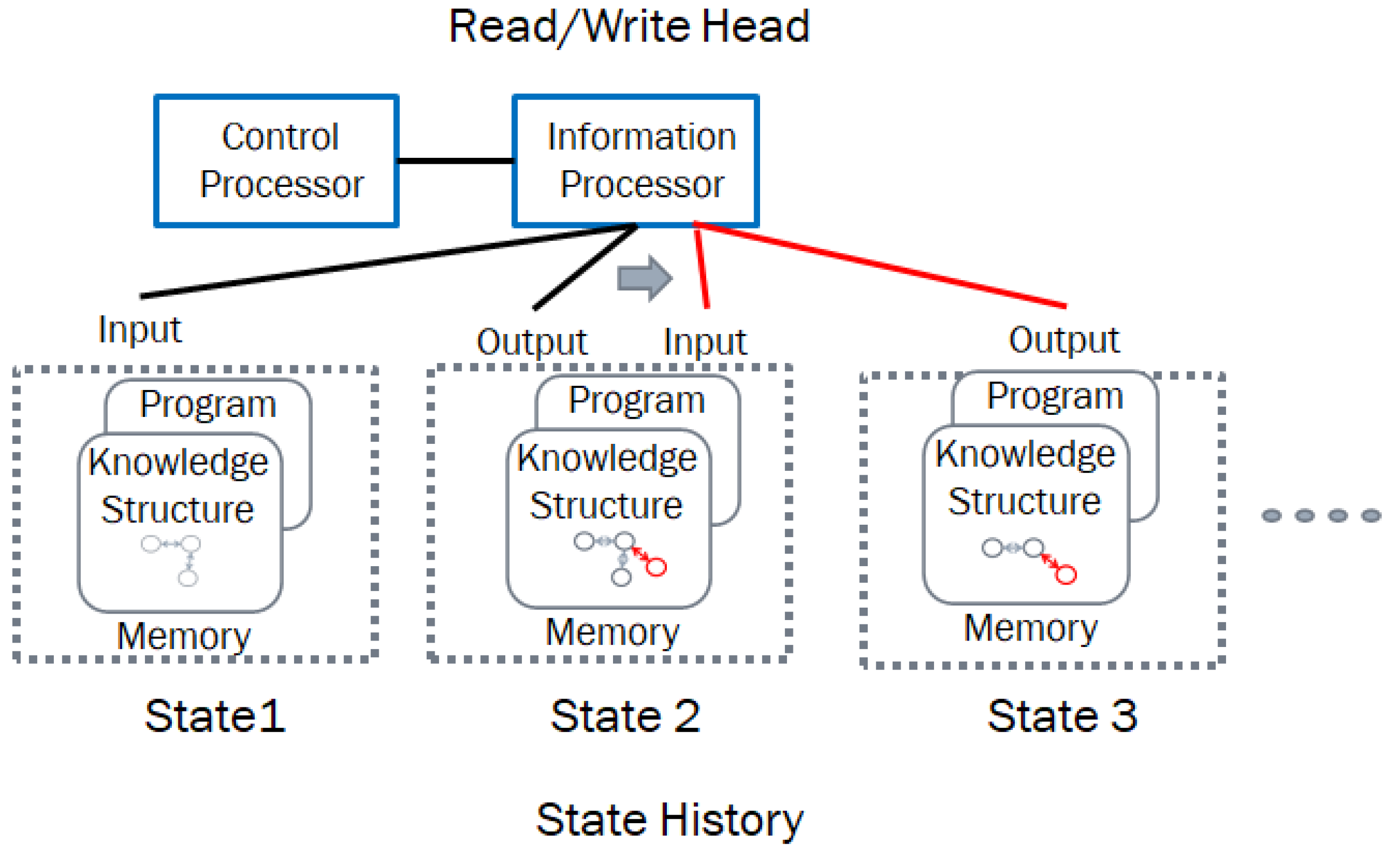
In this section we discuss how the use of new theory about knowledge structures, triadic automata, and structural machines allow us to design a new class of distributed information processing structures that use infware containing hierarchical intelligence to model, manage, and monitor distributed information processing hardware and software components as an active graph representing a network of networked processes. The infware, i.e., the processed information in the form of data structures, uses the operations on the schema representing the hardware, software, and their evolutionary behaviors as dynamic knowledge structures. An autopoietic system [32,33] implemented using triadic structural machines, i.e., structural machines working as triadic automata, is capable “of regenerating, reproducing, and maintaining itself by production, transformation, and destruction of its components and the networks of processes downstream contained in them.” The autopoietic machines discussed in this paper, which operate on schema containing knowledge structures, allow us to deploy and manage non-stop and highly reliable computing structures at scale independent of whose hardware and software are used. Figure 7 shows the structural machine operating on the knowledge structure in the form of an active graph in contrast to a data structure in the Turing machine implementation, which is a linear sequence of symbols.
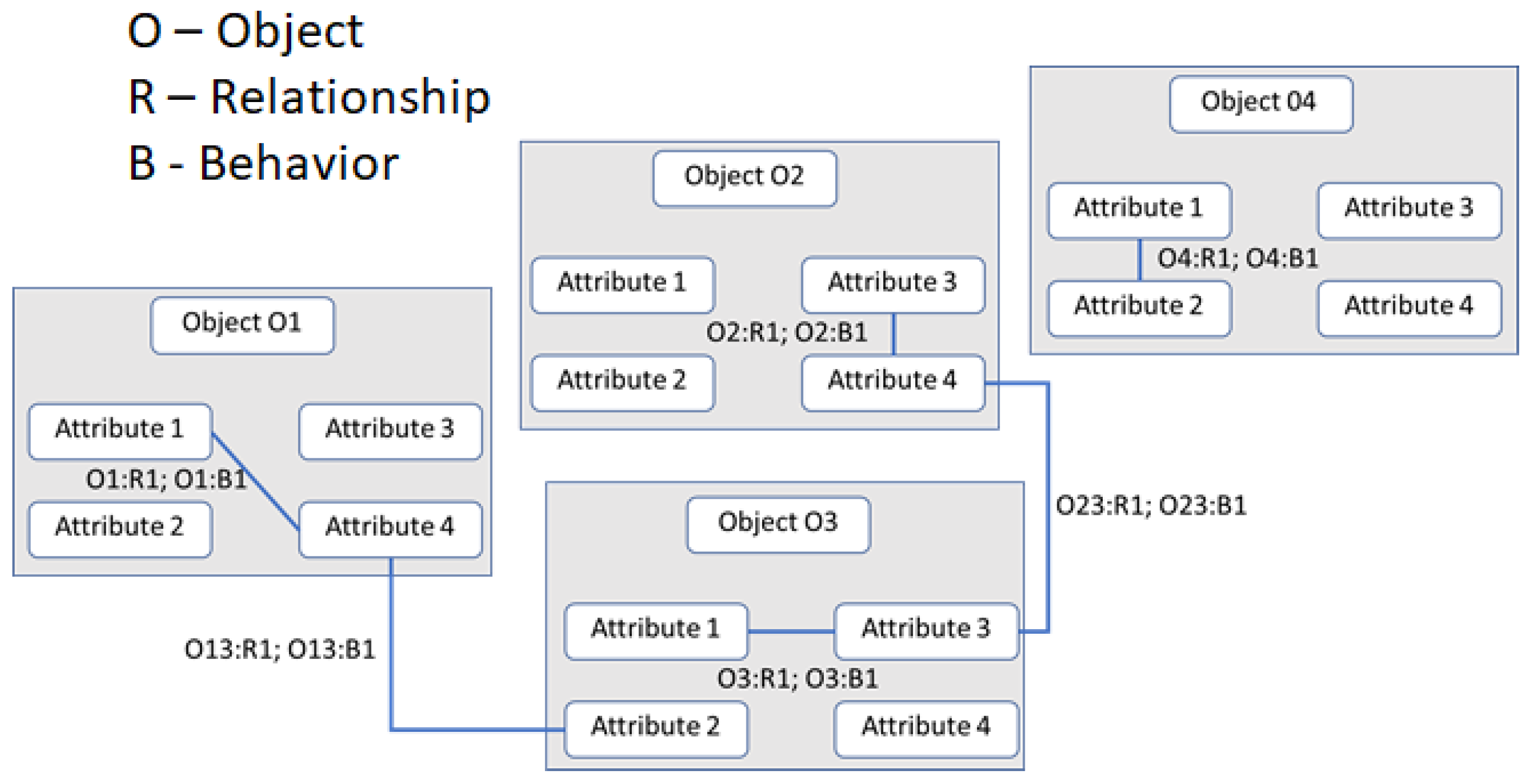
It is important to emphasize the differences between data, data structures, knowledge, and knowledge structures. Data are mental or physical “observables” represented as symbols. Data structures define patterns of the relationships between data items. Knowledge is a system that includes data enhanced by relations between the data and the represented domain. Knowledge structures include data structures abstracted to various systems and inter-object and intra-object relationships and behaviors, which emerge when an event occurs, changing the objects or their relationships. The corresponding state vector defines a named set of knowledge structures, a representation of which is illustrated in Figure 8.
Information processing in triadic structural machines is accomplished through operations on knowledge structures, which are graphs representing nodes, links, and their behaviors. Knowledge structures contain named sets and their evolution containing named entities/objects, named attributes, and their relationships. Ontology-based models of domain knowledge structures contain information about known knowns, known unknowns, and processes for dealing with unknown unknowns through verification and consensus. Inter-object and intra-object behaviors are encapsulated as named sets and their chains. Events and associated behaviors are defined as algorithmic workflows, which determine the system’s state evolution.
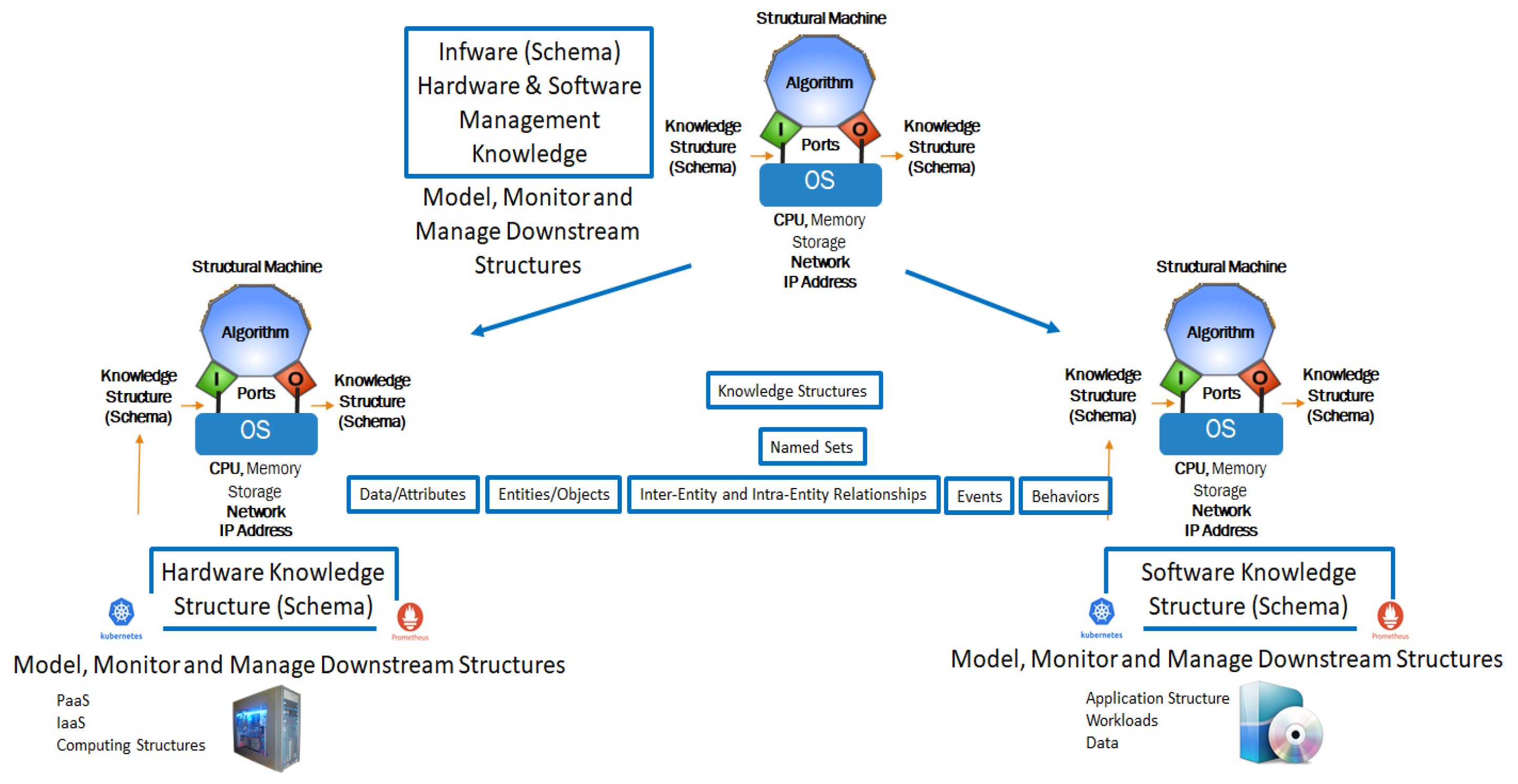
A named set chain of knowledge structures provides a genealogy representing the system state history. This genealogy can be treated as the deep memory and used for reasoning about the system’s behavior, as well as for its modification and optimization. In Figure 8, the behaviors are executed when an event induces a change. For instance, when Attribute 1 in Object 1 changes the behavior when B1 is executed, it in turn may cause another behavior workflow. In this paper, we use the knowledge structures to represent the schema that models how both hardware and software are configured, monitored, and managed during the evolution of computations, executing an information processing structure such as a business application. Figure 9 shows the implementation of the autopoietic machine with hardware, software, and infware, which is used to execute a business application.
The structural machine’s control processor operates on the downstream knowledge structures to evolve their states based on the event flow. At the leaf node, the conventional Turing automata operate on the data structures to evolve traditional computing processes. The important innovation here is the regulatory overlay to discover/configure, monitor, and manage the traditional computing process evolution using the local knowledge of how the local IaaS and PaaS are configured, monitored, and managed while coordinating with global knowledge to optimize the end-to-end system behavior in the face of fluctuations.
The schema in Figure 9 describes the hardware components, software components, and their management characteristics defined by knowledge structures, forming an autopoietic automaton. The knowledge structures represent this schema in the form of a system of named sets containing various data elements, objects, or entities that are composed of the data, and their inter-object and intra-object relationships and behaviors associated with events that cause changes to the instances as time progresses [27].
6. Conclusions
In this paper, we describe theoretical and practical computational tools for working with knowledge structures, such as schemas, taking into account their inter- and intra-relationships and associated behaviors when events change the state. We use triadic structural machines described in this paper to perform operations with schemas. The result is the design and implementation of autopoietic automata that are capable of regenerating, reproducing, and maintaining themselves by production, transformation, and destruction of its components and the networks of processes generated by them. Based on autopoietic automata and triadic structural machines working with schemas, we are currently building a system that models, monitors, and manages a distributed application deployed over multiple cloud resources to respond to large fluctuations in the demand for or the availability of computing resources in the system without disturbing the end to end transaction being delivered by the computing structure.
It is important to point out the difference between the current state of the art based on the classical computer science (constrained by the Church Turing thesis boundaries), which process information in the form of symbol sequences, and the current advancement of the field based on structural machines, which process information in the form of a dynamically-evolving network of networks represented by various schemas. As a result, we obtain autopoietic machines, which are capable of regenerating, reproducing, and maintaining themselves. The control processors in an autopoietic machine operate on the downstream graphs where a transaction can span across multiple distributed graphs, reconfiguring their nodes, links, and topologies based on well-defined pre-condition and post-condition transaction rules to address fluctuations, for example in resource availability or demand. The information processor of the machine, on the other hand, evolves the application workloads using the algorithms specified as programs operating on symbolic data structures.
Triadic structural machines provide the theoretical means for the design of autopoietic automata, whereas Turing machines cannot do this. The hierarchical control process overlay allows for the implementation of 4E (embedded, embodied, enactive, and extended) cognitive processes with downstream autonomous components interacting with each other and with their environment using system-wide knowledge-sharing, which allows global regulation to optimize the stability of the system as a whole based on memory and historical experience-based reasoning. This observation points out a major breakthrough in the way we will design future information processing systems with hierarchical intelligence and resilience at scale. We conclude this paper with the following observation from Leonardo da Vince: “He who loves practice without theory is like the sailor who boards ship without a rudder and compass and never knows where he may cast”.
Other applications of the constructions and results of this paper are described in other papers of the authors and other researchers.
Author Contributions
Both authors have equally contributed to the article, its conceptualization, methodology, investigation, writing, original draft preparation, review, and editing. All authors have read and agreed to the published version of the manuscript.
Funding
This research received no external funding.
Data Availability Statement
The study does not report any data.
Conflicts of Interest
The authors declare no conflict of interest.
References
- Burgin, M. Theory of Information: Fundamentality, Diversity and Unification; World Scientific: New York, NY, USA; London, UK; Singapore, 2010. [Google Scholar]
- Minsky, M. The Society of Mind; Simon and Schuster: New York, NY, USA, 1986. [Google Scholar]
- Burgin, M. Theory of Knowledge: Structures and Processes; World Scientific: New York, NY, USA; London, UK; Singapore, 2016. [Google Scholar]
- Arbib, M.A. Modules, Brains and Schemas. In Formal Methods in Software and Systems Modeling. Lecture Notes in Computer Science; Kreowski, H.J., Montanari, U., Orejas, F., Rozenberg, G., Taentzer, G., Eds.; Springer: Berlin/Heidelberg, Germany, 2005; Volume 3393. [Google Scholar]
- Kant, I. Critique of Pure Reason; Smith, N.K., Translator; Macmillan: London, UK, 1929. [Google Scholar]
- Head, H.; Holmes, G. Sensory Disturbances from Cerebral Lesions. Brain 1911, 34, 102–254. [Google Scholar] [CrossRef] [Green Version]
- Bartlett, F.C. Remembering; Cambridge University Press: Cambridge, UK, 1932. [Google Scholar]
- Piaget, J. The Language and Thought of the Child; Kegan Paul, Trench &Trubner: London, UK, 1926. [Google Scholar]
- Elmasri, R.; Navathne, S.B. Fundamentals of Database Systems; Addison-Wesley: Reading, MA, USA, 2000. [Google Scholar]
- Daum, B. Modeling Business Objects with XML Schema; Morgan Kauffman: Burlington, MA, USA, 2003. [Google Scholar]
- Duckett, J.; Ozu, N.; Williams, K.; Mohr, S.; Cagle, K.; Griffin, O.; Francis Norton, F.; Stokes-Rees, I.; Tennison, J. Professional XML Schemas; Wrox Press Ltd.: Birmingham, UK, 2001. [Google Scholar]
- Gowri, K. EnrXML–A Schema for Representing Energy Simulation Data. In Proceedings of the 7th International IBPSA Conference, Rio de Janeiro, Brazil, 13–15 August 2001; pp. 257–261. [Google Scholar]
- Ershov, A.P. Mixed Computation in the Class of Recursive Program Schemata. Acta Cybern. 1980, 4, 19–23. [Google Scholar]
- Ianov, Y.I. On the Equivalence and Transformation of Program Schemes. Commun. ACM 1958, 1, 8–12. [Google Scholar] [CrossRef]
- Karp, R.M.; Miller, R.E. Parallel Program Schemata. J. Comput. Syst. Sci. 1969, 3, 147–195. [Google Scholar] [CrossRef] [Green Version]
- Keller, R.M. Parallel Program Schemata and Maximal Parallelism. JACM 1973, 20, 514–537. [Google Scholar] [CrossRef]
- Dennis, J.B.; Fossen, J.B.; Linderman, J.P. Data Flow Schemes; LNCS, 19; Springer: Berlin/Heidelberg, Germany, 1974. [Google Scholar]
- Arbib, M.A. Schema Theory. In The Encyclopedia of Artificial Intelligence, 2nd ed.; Shapiro, S., Ed.; Wiley-Interscience: Hoboken, NJ, USA, 1992; pp. 1427–1443. [Google Scholar]
- Price, E.; Driscoll, M. An Inquiry into the Spontaneous Transfer of Problem-Solving Skill. Contemp. Educ. Psychol. 1997, 22, 472–494. [Google Scholar] [CrossRef] [PubMed]
- Solso, R.L. Cognitive Psychology; Allyn and Bacon: Boston, MA, USA, 1995. [Google Scholar]
- Cole, M.I. Algorithmic Skeletons; MIT Press: Cambridge, MA, USA, 1989. [Google Scholar]
- Schank, R.C.; Abelson, R.P. Scripts, Plans. In Goals and Understanding; Lawrence Erlbaum Associates: Hillsdale, NJ, USA, 1977. [Google Scholar]
- Burgin, M. Mathematical Models in Schema Theory. arXiv 2005, arXiv:cs/0512099. [Google Scholar]
- Burgin, M. From Craft to Engineering: Software Development and Schema Theory. In Proceedings of the 2009 WRI World Congress on Computer Science and Information Engineering (CSIE 2009), WRI, Los Angeles, CA, USA, 31 March–2 April 2 2009; Volume 7, pp. 787–791. [Google Scholar]
- Burgin, M. Mathematical Schema Theory for Network Design. In Proceedings of the ISCA 25th International Conference on Computers and their Applications (CATA-2010), ISCA, Honolulu, HI, USA, 24–26 March 2010; pp. 157–162. [Google Scholar]
- Burgin, M. Information Processing by Structural Machines, in Theoretical Information Studies: Information in the World; World Scientific: New York, NY, USA; London, UK; Singapore, 2020; pp. 323–371. [Google Scholar]
- Mikkilineni, R.; Burgin, M. Structural Machines as Unconventional Knowledge Processors. Proceedings 2020, 47, 26. [Google Scholar] [CrossRef]
- Burgin, M. From Neural Networks to Grid Automata. In Proceedings of the IASTED International Conference Modeling and Simulation, Palm Springs, CA, USA, 9–11 April 2003; pp. 307–312. [Google Scholar]
- Burgin, M. Cluster Computers and Grid Automata. In Proceedings of the ISCA 17th International Conference on Computers and Their Applications (CATA-2002), San Francisco, CA, USA, 4–6 April 2002. [Google Scholar]
- Burgin, M. Super-Recursive Algorithms; Springer: New York, NY, USA; Berlin/Heidelberg, Germany, 2005. [Google Scholar]
- Burgin, M. Super-Recursive Algorithms and Modes of Computation. In Proceedings of the 2015 European Conference on Software Architecture Workshops, Dubrovnik/Cavtat, Croatia, 7–11 September 2015; pp. 10:1–10:5. [Google Scholar]
- Burgin, M.; Mikkilineni, R.; Phalke, V. Autopoietic Computing Systems and Triadic Automata: The Theory and Practice. Adv. Comput. Commun. 2020, 1, 16–35. [Google Scholar] [CrossRef]
- Maturana, H.R.; Varela, F.J. Autopoiesis and Cognition. The Realization of the Living; Reidel: Dordrecht, The Netherlands, 1980. [Google Scholar]
Figure 1.
A schema of transducer hardware.

Figure 2.
A schema of parallel information processing device hardware.

Figure 3.
A schema of a Turing machine.

Figure 4.
A schema of an inductive Turing machine.

Figure 5.
A schema of the transducer hardware.

Figure 6.
Data and the program stored in the computer memory are processed by the CPU in the information processor.
Figure 6.
Data and the program stored in the computer memory are processed by the CPU in the information processor.

Figure 7.
The schema with a triadic automaton represents a knowledge structure containing various object, inter-object, and intra-object relationships and behaviors, which emerge when an event occurs, changing the objects or their relationships.
Figure 7.
The schema with a triadic automaton represents a knowledge structure containing various object, inter-object, and intra-object relationships and behaviors, which emerge when an event occurs, changing the objects or their relationships.

Figure 8.
A knowledge structure modeling intra-object and inter-object behaviors.

Figure 9.
Schema managing infware, hardware, and software for the deployment, configuring, monitoring, and managing distributed application workloads on cloud resources.
Figure 9.
Schema managing infware, hardware, and software for the deployment, configuring, monitoring, and managing distributed application workloads on cloud resources.

Publisher’s Note: MDPI stays neutral with regard to jurisdictional claims in published maps and institutional affiliations. |
© 2021 by the authors. Licensee MDPI, Basel, Switzerland. This article is an open access article distributed under the terms and conditions of the Creative Commons Attribution (CC BY) license (http://creativecommons.org/licenses/by/4.0/).
Share and Cite
MDPI and ACS Style
Burgin, M.; Mikkilineni, R. From data Processing to Knowledge Processing: Working with Operational Schemas by Autopoietic Machines. Big Data Cogn. Comput. 2021, 5, 13. https://0-doi-org.brum.beds.ac.uk/10.3390/bdcc5010013
AMA Style
Burgin M, Mikkilineni R. From data Processing to Knowledge Processing: Working with Operational Schemas by Autopoietic Machines. Big Data and Cognitive Computing. 2021; 5(1):13. https://0-doi-org.brum.beds.ac.uk/10.3390/bdcc5010013
Chicago/Turabian StyleBurgin, Mark, and Rao Mikkilineni. 2021. "From data Processing to Knowledge Processing: Working with Operational Schemas by Autopoietic Machines" Big Data and Cognitive Computing 5, no. 1: 13. https://0-doi-org.brum.beds.ac.uk/10.3390/bdcc5010013