Article

Automatic Defects Segmentation and Identification by Deep Learning Algorithm with Pulsed Thermography: Synthetic and Experimental Data

by
Qiang Fang
*,
Clemente Ibarra-Castanedo
and
Xavier Maldague
*
Computer Vision and Systems Laboratory, Department of Electrical and Computer Engineering, Université Laval, 1065, av. de la Médecine, Québec, QC G1V 0A6, Canada
*
Authors to whom correspondence should be addressed.
Big Data Cogn. Comput. 2021, 5(1), 9; https://0-doi-org.brum.beds.ac.uk/10.3390/bdcc5010009
Submission received: 29 December 2020 / Revised: 19 February 2021 / Accepted: 19 February 2021 / Published: 26 February 2021
(This article belongs to the Special Issue Machine Learning and Data Analysis for Image Processing)

Abstract

:
In quality evaluation (QE) of the industrial production field, infrared thermography (IRT) is one of the most crucial techniques used for evaluating composite materials due to the properties of low cost, fast inspection of large surfaces, and safety. The application of deep neural networks tends to be a prominent direction in IRT Non-Destructive Testing (NDT). During the training of the neural network, the Achilles heel is the necessity of a large database. The collection of huge amounts of training data is the high expense task. In NDT with deep learning, synthetic data contributing to training in infrared thermography remains relatively unexplored. In this paper, synthetic data from the standard Finite Element Models are combined with experimental data to build repositories with Mask Region based Convolutional Neural Networks (Mask-RCNN) to strengthen the neural network, learning the essential features of objects of interest and achieving defect segmentation automatically. These results indicate the possibility of adapting inexpensive synthetic data merging with a certain amount of the experimental database for training the neural networks in order to achieve the compelling performance from a limited collection of the annotated experimental data of a real-world practical thermography experiment.

1. Introduction

Quality evaluation is playing a fundamental role for modern industrial production and manufacturing processing. The demand for the inspection of materials with respect to the possible presence of defects, damage, and flaws has increased due to the wide use of composite materials and metals in industries such as aerospace. The method used to inspect defects via manual, visual evaluation involving humans can be hampered by the human fatigue and subjectivity. In order to meet the need of high-quality production and maintain the stringent high-quality level, an advanced inspection system is becoming more and more essential for structural health monitoring and production lines application. Automated quality control [1] can be applied in the industrial field to facilitate the consistent and efficient inspection. The high inspection rate and the inspection procedure without human involvement are the main advantages of automated inspection systems [2].
Non-Destructive Testing (NDT) [3] encompasses a group of inspection techniques that are intended to assess the integrity of an object without causing any kind of modification or permanent damage. Infrared testing (IRT) is an NDT technique in which the differences in thermo-physical properties between the inspected object sound material and possible surface and/or subsurface defects are exploited through the use of an infrared camera. However, automatically identifying defects in materials via IRT still remains an ongoing and challenging task in the image processing domains.
For the defect identification and detection, several state-of-the-art defect detection algorithms have been proposed in previous literature. These included Faster-Region based Convolutional Neural Networks (Faster-RCNN) [4], YOLO-V3 [5], Autoencoders structured neural network [6], and conditional monitoring (CM)-based feature learning methods [7,8]. Faster-RCNN and YOLO-V3 detectors were used to automatically localize flaws in a thermography diagnosis system. These methods show satisfied performance on the defect localization when multi-properties were contained in defect information. However, some issues still need to be improved for the whole marking process in these methods. For example, bounding boxes from YOLO-V3 and Faster-RCNN offer some restrictions in most cases, although they are fast and easy to localize. The area of non-defect always occupied a high percentage of area from bounding boxes, which may possibly introduce multiple errors during the whole training process. The Autoencoders structured neural network [6] was proposed as an unsupervised learning method to automatically extract features from intelligent faults. This method has made impressive research progress during the thermography data processing. However, the encoder–decoder format (Autoencoders structured) algorithm may have unavoidable limitations in faults extraction from thermographic data processing due to weakness signals, complex noise interference, data limitation, etc. The regular CM based-feature learning methods derived from the idea of Convolutional Neural Network (CNN) feature transformations and transfer learning [9], which have shown strong capability as a pattern to detect the flaws or defect location naturally and obtained an excellent performance. Due to the data limitation as well as high noise inference from the experimental infrared thermal databases, it is still quite complicated to train a model that has strong robustness to detect irregular and complex flaws in the CM defect diagnosis system.
Therefore, in this research, an automatic instance segmentation and identification algorithm in deep learning (Mask-RCNN) [10] is introduced for defect segmentation in an automatic infrared detection system. The defect detection procedure can be regarded as either an object detection task [11] or object segmentation task [12]. In the object detection task, the objective is to fit the bounding box localized around each defect in the image. In the object segmentation task, the objective is based on pixel-level classification to distinguish each pixel if it is detected. Compared with the earlier segmentation strategies [13,14], the Instance segmentation associated each pixel of an image with an instance label [15]. It can predict a whole segmentation mask for each of those objects and predict accurately which pixel in the input image corresponds to each object instance. It also reduces the restriction concerning the position of defects rather than predicting a group of bounding boxes for the defects.
Meanwhile, as discussed in the state-of-the-art approach [7,8], deep learning’s Achilles heel is the training dataset. The training dataset must be accurate enough and contain enough images and exceptions (e.g., occlusions) so as to allow the algorithm to learn reliable features of interest. If the dataset does not contain enough images and cases of possible situations or if the data contain too much noise or artifacts, the algorithm may not be accurate enough or even may learn to identify the wrong features (in the cases of CM feature learning methods). During recent years, the exploitation of synthetic data [16] during the training and validation of deep neural networks has emerged as a popular topic. In this work, synthetic data generated with Finite Element Models (FEM) is used during the training process to greatly reduce the high expenses involved in real experiments in infrared thermography. The synthetic data generated by the simulator are based on the same parameters with real specimens in non-realistic ways, being able to force the neural network to learn the essential features of the object of interest [17]. The generated features from synthetic data can cover or overlap the amount of data distribution that are not sufficiently represented in the original experimental dataset [18]. The results also show the possibility of using inexpensive synthetic data for the deep neural network training but avoiding the necessity of collecting large amounts of hand-annotated experimental data.
In this research, a small amount of IRT experimental data together with FEM synthetically generated IRT data will be used to train a deep spatial characteristic model (Mask-RCNN) for the segmentation of defects. This proposed method can effectively achieve the defect identification and segmentation with the cases of data limitation. The contribution of this work can be illustrated in the following:
(1)
By adapting a data augmentation strategy through the Synthetic Data Generation Pipeline (Finite Element Modeling), the proposed method effectively improves the performance of segmentation (capability for feature extraction as well as reducing the noise interference).
(2)
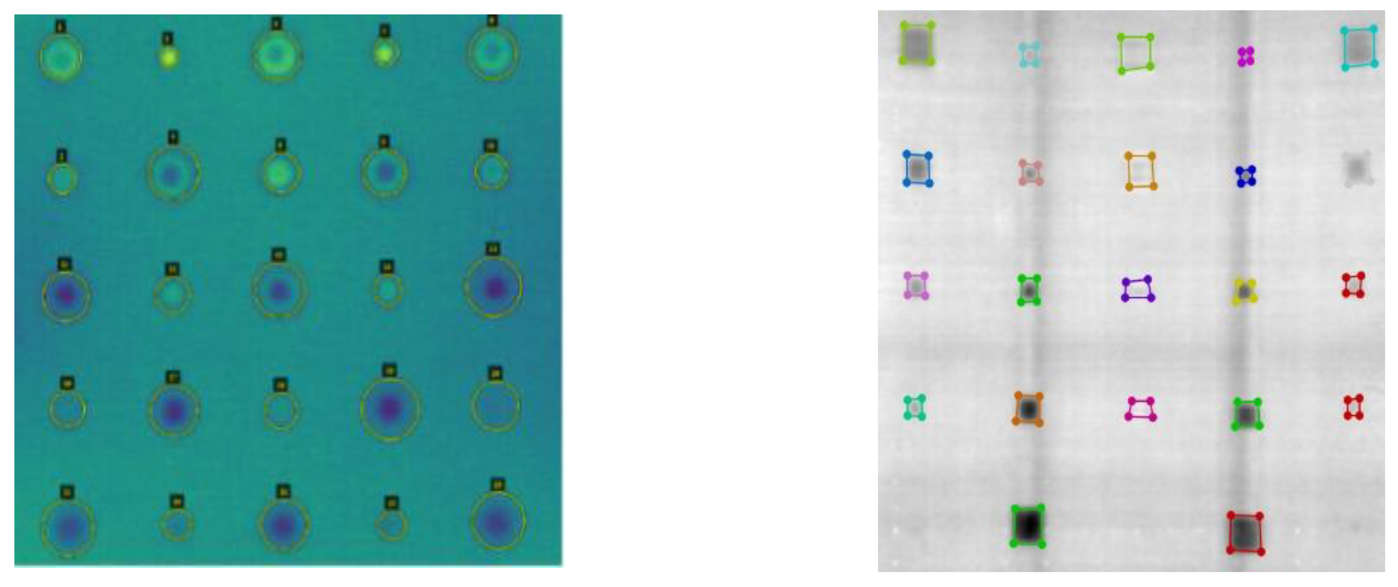
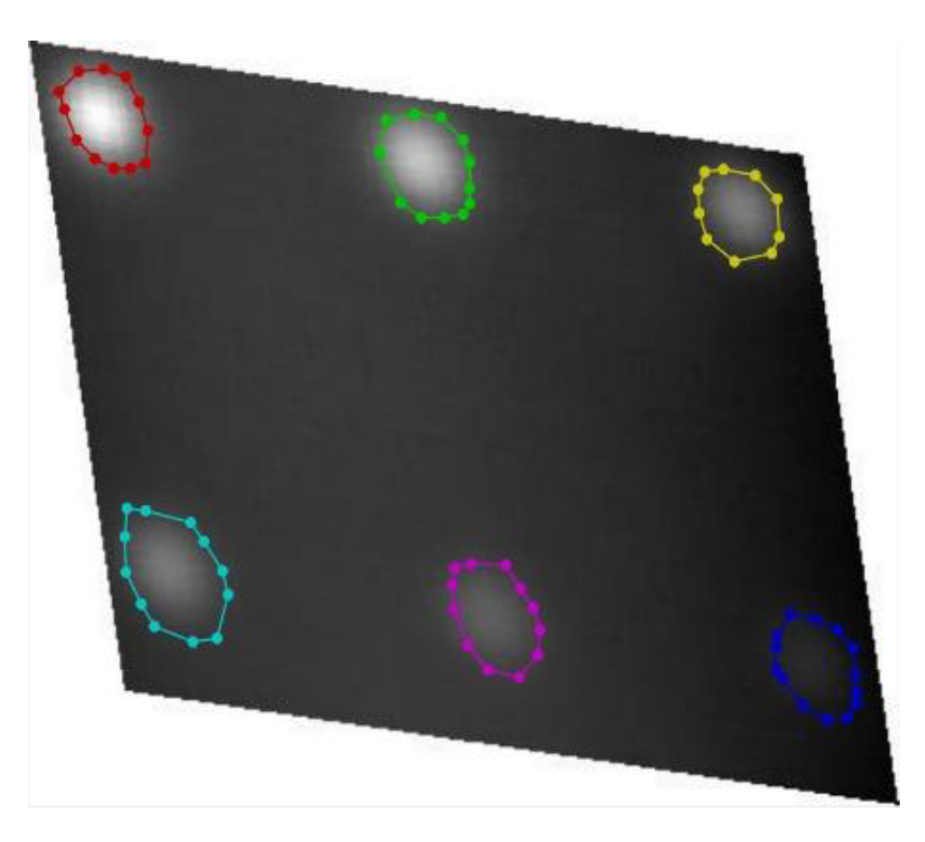
An instance segmentation is introduced for defects segmentation and identification for each object of defects with different specimens to predict each irregular shape of defects instance in the input images at the pixel’s level.
The remainder of the paper is structured as follows: Section 2 provides the pulsed thermography and related experimental set-up. Section 3 gives a detailed explanation of the Mask-RCNN defects detection system and the synthetic data generation pipeline. Section 4 describes the main features and dataset for evaluation. Section 5 provides the experimental results and implementation stages, including the comparison with states-of-the-art object detection algorithms (YOLO-V3; Faster-RCNN). Section 6 furtherly discusses and analyzes experimental results. Section 7 concludes this paper.

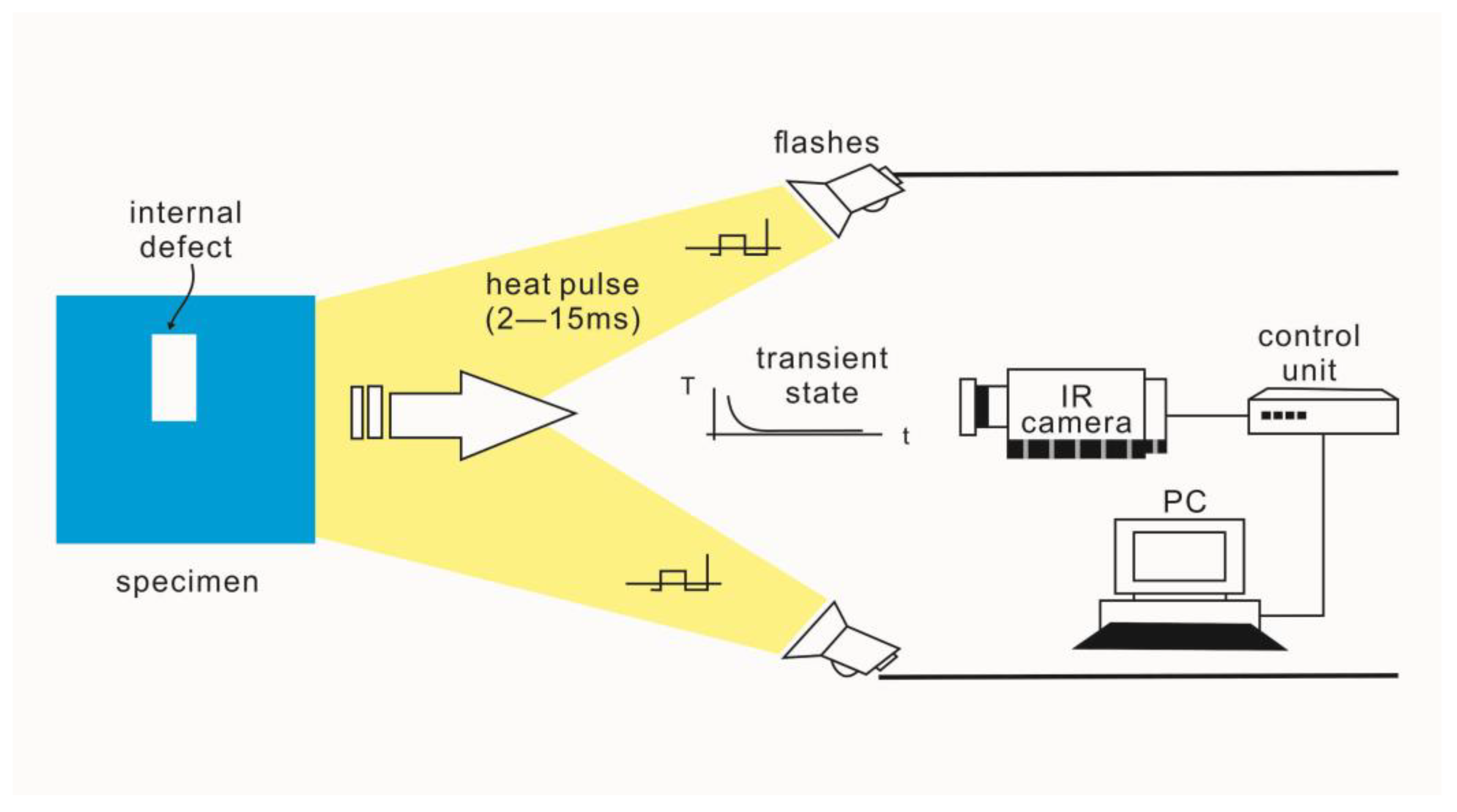
2. Thermophysical Consideration

In pulsed thermography (PT), the surface of the inspected specimen is exposed to a heat pulse using an energy source such as photographic flashes, as indicated in Figure 1. A heat pulse can be represented as the combination of several periodic waves having different frequencies and amplitudes. After the thermal front reaches the surface of the specimen, a thermal front travels from the surface through the specimen. As time elapses, the normal path of the thermal front changes due to the presence of the subsurface discontinuity, and leads to the thermal contrast at the specimen’s surface, which can be monitored with an infrared (IR) camera. The one-dimensional solution of the Fourier equation of conduction for a Dirac heat pulse propagating through a semi-infinite isotropic solid has the form [19]:
T ( z , t ) = T 0 + Q k p c t e ( z 2 4 α t )
where Q [ J / m 2 ] is the energy absorbed from the surface, and the initial temperature is T 0   [ K ] . p   [ kg / m 3 ] is density. The specific heat at constant pressure is c   [ J / kgK ] . K   [ W / mK ] is the thermal conductivity that indicated the energy transformation rate by the materials. α   [ m 2 /s] is the thermal diffusivity to measure the material ability to conduct heat, and Z [mm] is the depth of the defect. At the surface (z = 0), the temperature evolution can be written as follows [20]:
T ( 0 , t ) = T 0 + Q k p c t
From Equation (2), it can be concluded that the temperature evolution at the surface following a Dirac heat pulse follows a monotonous decrease with a slope of −1/2 for areas without defects, whilst areas with defects will diverge more or less from this behavior depending on their actual thermo-physical properties.

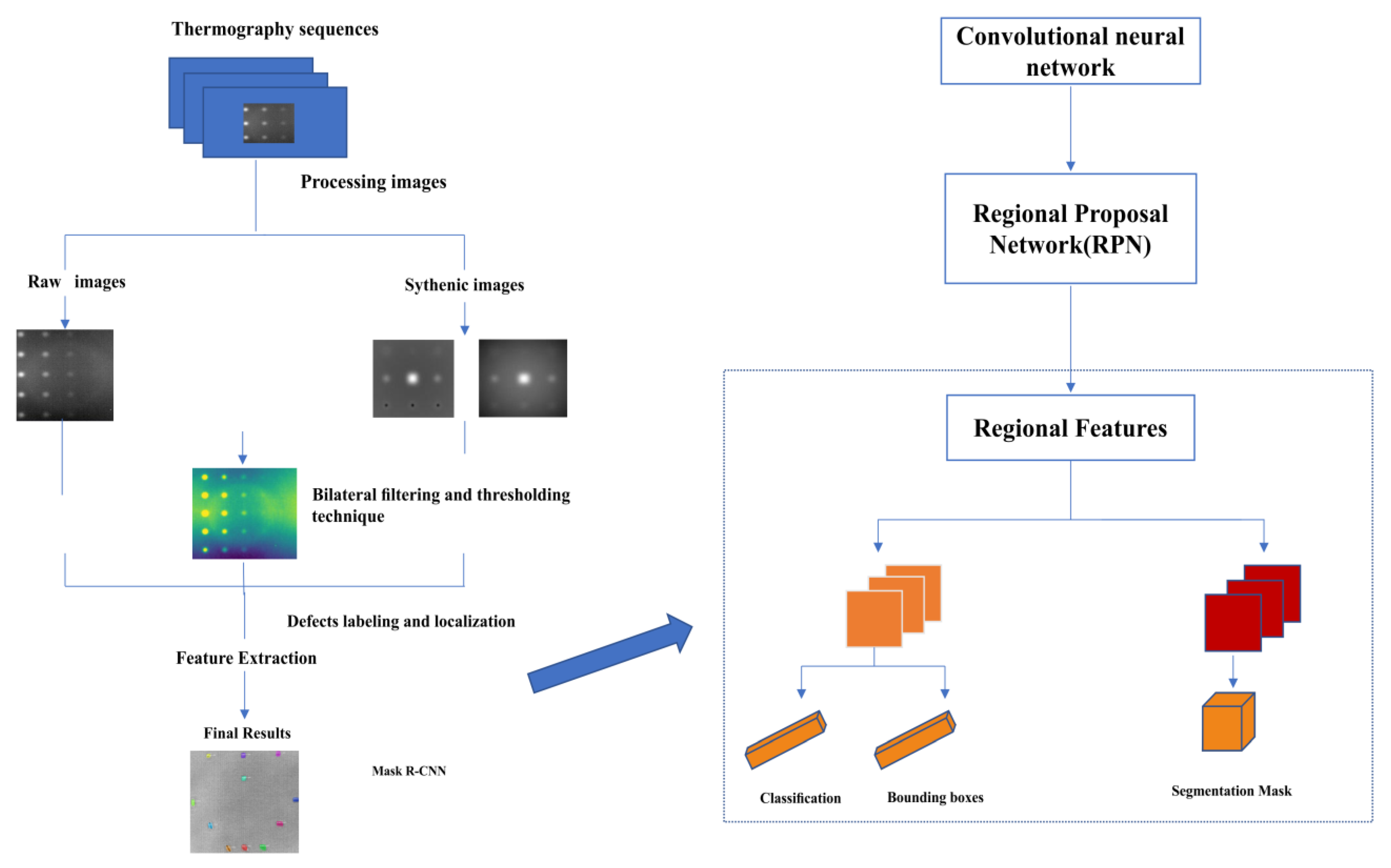
3. Automatic Defect Segmentation Strategy
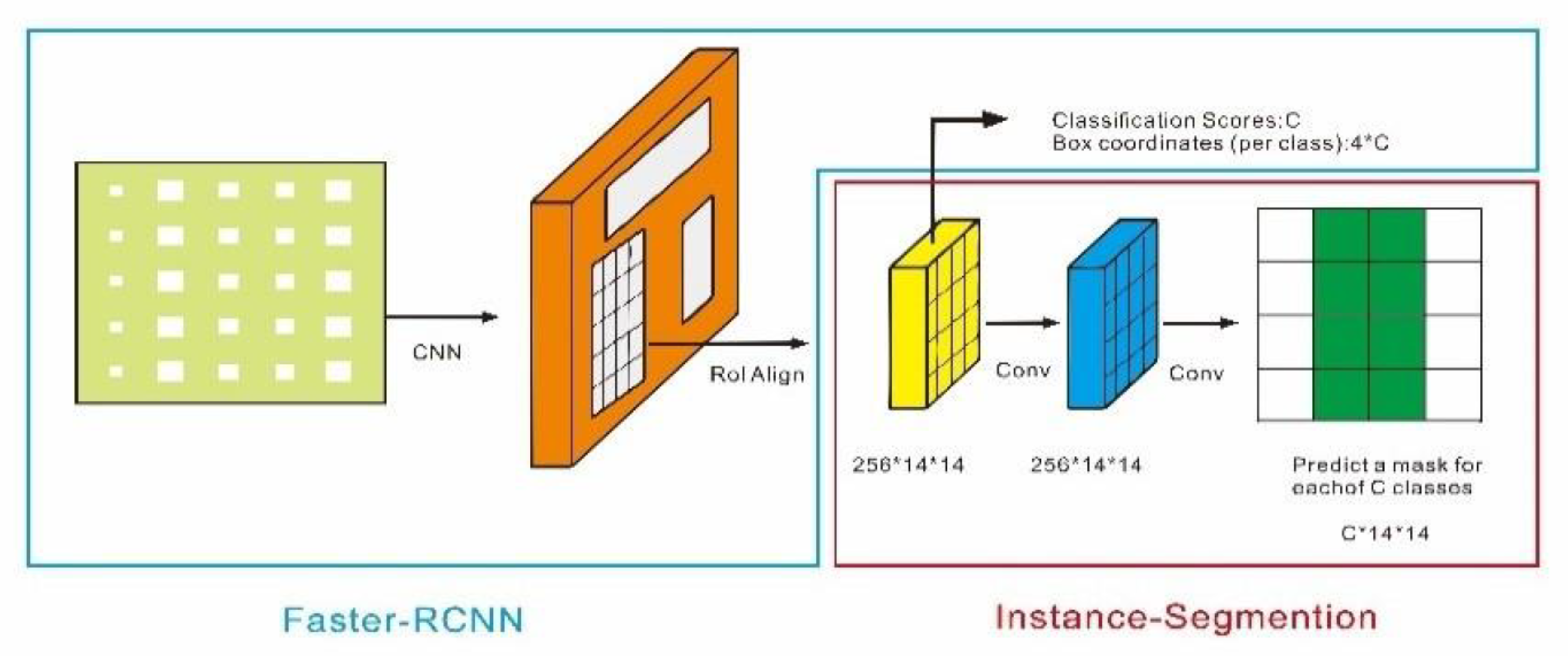
As indicated in Figure 2, a detection system training with, for most intents and purposes, data generated by a computer simulation can be seen as synthetic data; experimental data has been proposed to segment and identify defects in thermal images. This design of this detection system is based on Mask R-CNN. The infrared thermal sequences are acquired by pulsed thermography (PT). Then, both the raw and synthetic sequences are preprocessed with the bilateral filtering and the thresholding technique. Therefore, two different characteristic datasets (raw data; synthetic data) are generated respectively, to be trained with Mask-RCNN in different combination cases. In the final step, delamination is identified through the deep region convolutional neural network and then visualized with the bounding box or instance segmentation map.

3.1. Mask-RCNN

Convolutional Neural Networks (CNN) are utilized as a supervised feature extractor to analyze the defect localization and segmentation from materials. The Region based-CNN (R-CNN) [21] move toward the object bounding box detection method based on each region of interest (ROI). Faster-RCNN [11] have further advanced the network via learning the attention mechanism with a Region Proposal Network (RPN). Mask R-CNN [4] extends from Faster-RCNN through a mask branch construction. It is an instance segmentation algorithm, which recognizes object boundaries at the pixel level and designs pixel-wise segmentation with alignment of pixel-to-pixel among the input and output. Mask R-CNN adopts the same two-stage with Faster-RCNN architecture. During the first stages, the input images were scanned, and the proposals were generated via the Region Proposal Network (RPN). In the second stage of detection, it included two total branches. At the first branch (the blue line box at the top in the Figure 3), it predicted classification scores to tell what is the category corresponding to that region of proposal (whether or not it is background). Each of the bounding box coordinates that regressed off the region proposal coordinates was indicated. At the second branch (the red line box at the bottom in the Figure 3), it added a binary mask regarding each ROI as a mini semantic segmentation network [22] to classify for each pixel in that input region proposal whether or not it is an object. Mask R-CNN is intended to address the instance segmentation task and aims at adjusting the plentiful hyper-parameters from the neural network. This model predicts a certain number of bounding boxes for the defects, while each defect region is segmented within the bounding boxes at the same time. The architecture is shown in Figure 3. The loss function of Mask-RCNN in Equation (3) consists of five different terms:
  • RPN_class_loss: The performance of objects can be separated from background via RPN;
  • RPN_bounding_box_loss: The performance of RPN to specify the objects;
  • Mrcnn_bounding_box_loss: The performance of Mask R-CNN specifying objects;
  • Mrcnn_class_loss: The performance of classifying each class of object via Mask R-CNN;
  • Mrcnn_mask_loss: The performance of segmenting objects via Mask R-CNN.
In these five terms, when the cost loss values are smaller, then performance improves.
L c o s t = L _ ( r p n _ c l a s s ) +   L _ ( r p n _ b b o x ) + L _ ( m r c n n _ b b o x ) + L   _ ( m r c n n _ c l a s s ) + L _ ( m r c n n _ m a s k )

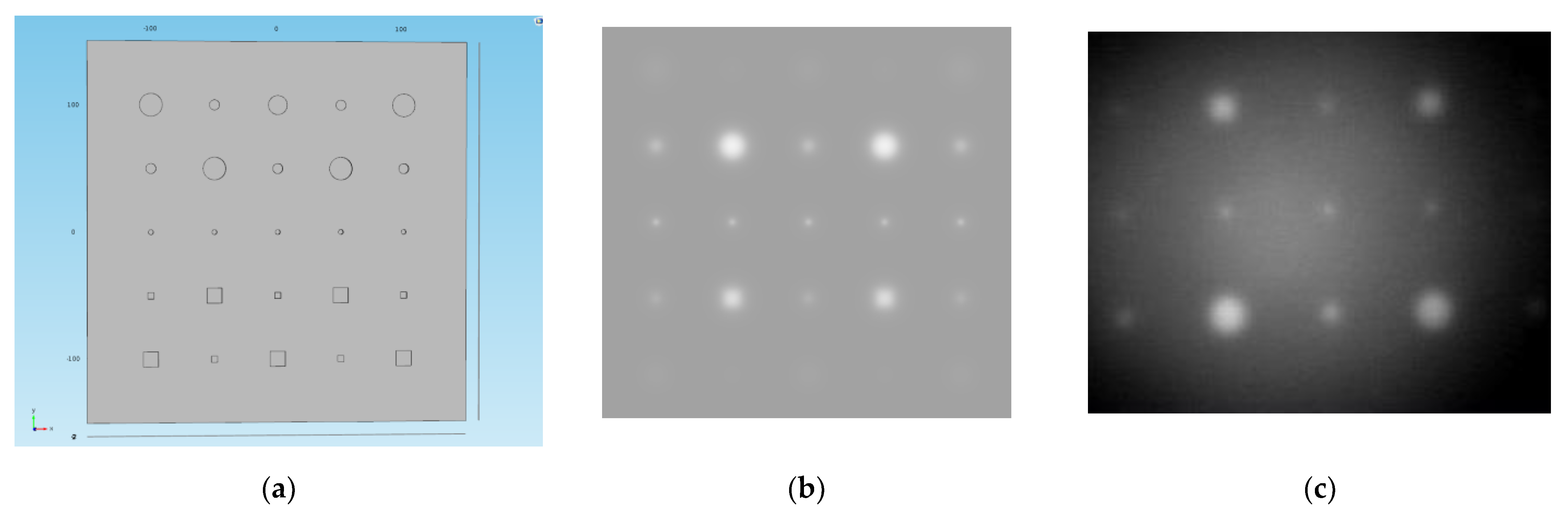
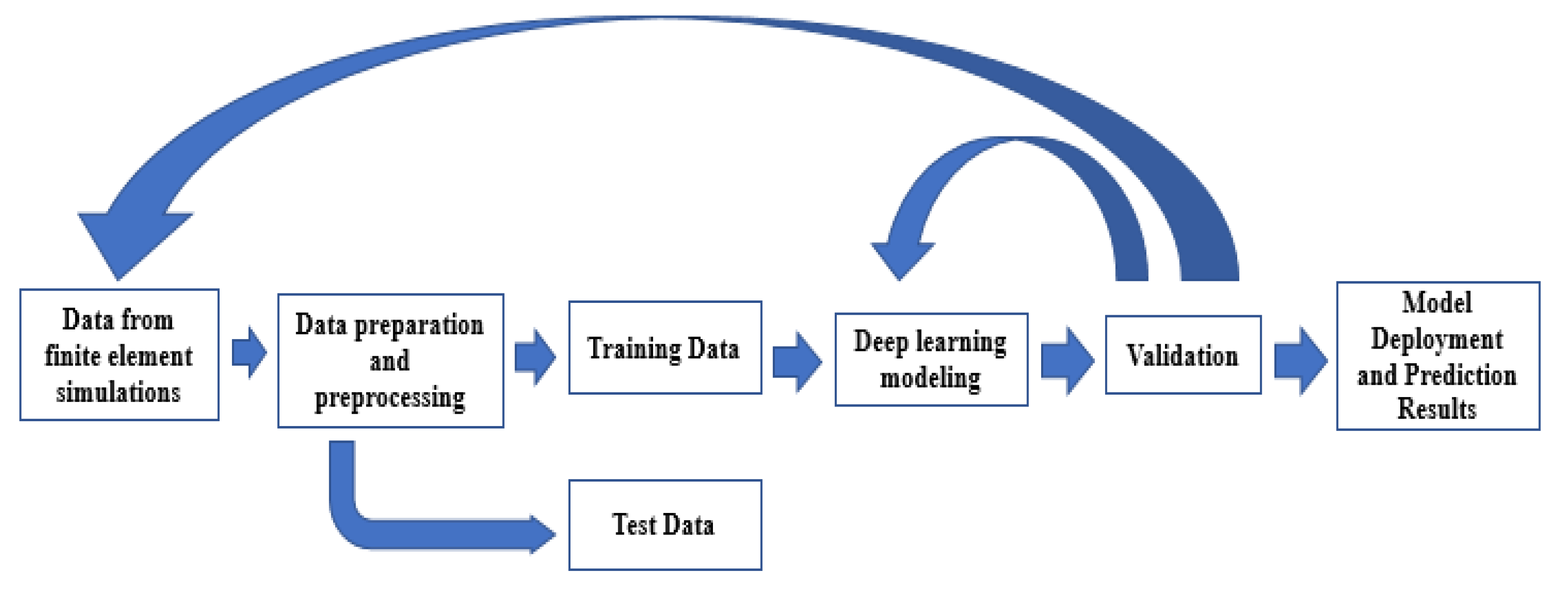
3.2. Synthetic Data Generation Pipeline

Synthetic data are computed information rather than data collected from real-word events [16]. The main application involves using synthetic data as a training dataset. The use of synthetic data provides several benefits; one of the most interesting is that it is possible to generate large databases to train, modify, and create new variables and features on individual data cases. Another advantage is that labeling is quite straightforward and precise.
Finite Element Modeling (FEM) has become a practical tool to evaluate the thermal response of pulsed thermography. It is also intended for predicting and simulating the results of Thermal NDT (Non-Destructive Testing) experiments and allows the solving of three-dimensional heat conduction problems in samples containing surface and subsurface defects. This plexiglass sample (30 cm × 30 cm) was designed with 25 flat bottom holes (FBH), which are located at increasing depths in either circles or square shapes, as indicated in Figure 4a. Figure 4b shows the pulsed thermography result of a plexiglass synthetic sample from FEM simulation at t = 106.5 s after heating, which indicates defects more distinctly compared to the corresponding experimental frame at the same time shown in Figure 4c. A good correspondence temperature of the region is observed, which verifies that synthetic modeling in FEM is in outstanding accordance with the real experiment [23]. The detailed implementation procedure for using deep neural networks with FEM is described in Figure 5. The training of synthetic data generated by FEM provides clean and automated supervision data compared to the other numerical methods such as boundary element methods [24] and finite volume methods [25], where most other numerical computational methods are highly non-linear and have uncertainty issues with respect to quantification and simulation. In addition, the learning process can be abundantly simplified since both synthetic and experimental data are governed by the same heat transfer principles. Specific feature positioning and extraction for less visible defect regions can be referenced from the synthetic data.

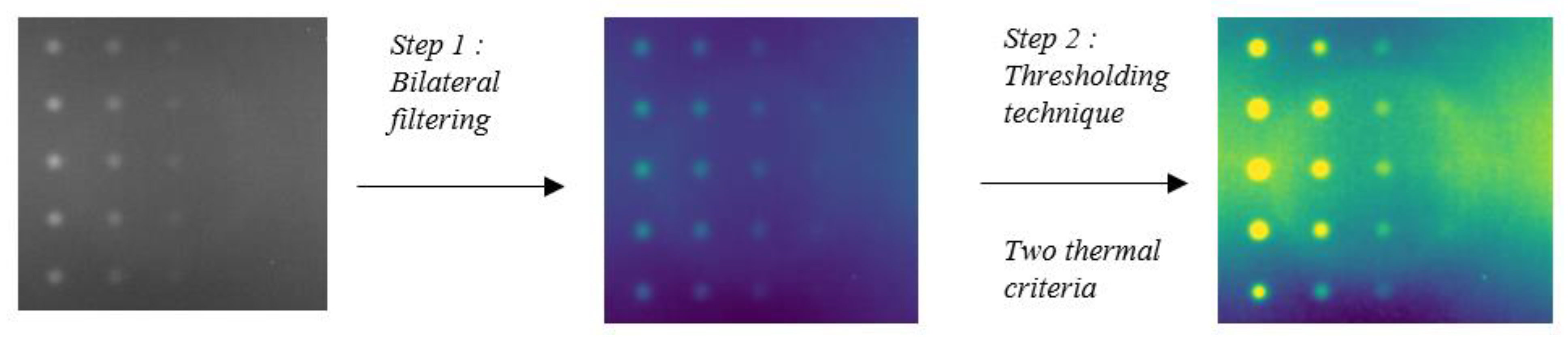
3.3. Automatic Preprocessing Stage

The main purposes of the preprocessing stage (Figure 6) are to make defects more distinguishable from the cluttered background of the thermal sequence and to normalize data. The bilateral filtering and thresholding techniques present in [26] were adapted for the preprocessed stage in this work so as to be the reference database. In step 1, the bilateral filtering removes noise from the thermal image while preserving feature edges. Secondly, two thermal criteria are applied in a thermal image sequence acquired from pulsed thermography: (1) 1st thermal criterion: automatically determine the instant just before the appearance of the first thermal footprint belonging to a defect (reference point); (2) 2nd thermal criterion: automatically find the intersection point between the overlap of each of the thermal image histograms after the reference point and the thermal image histogram corresponding to the reference point. In the end, the pixel values above the corresponding intersection point are equal to this value. Pixel values corresponding to the thermal images after the reference point are multiplied by a scale in Equation (4). The final result of this method is believed to be fitted with the convolutional neural network stage thereafter.
S c a l e   V a l u e = ( M a x _ p i x e l _ v a l u e     M i n _ p i x e l _ v a l u e ) c o r r e s p o n d i n g   t o   t h e   n   t h e r m a l   a f t e r   S t e p 1 ( i n t e r s e c t i o n   p o i n t     M i n _ p i x e l _ v a l u e ) c o r r e s p o n d i n g   t o   t h e   n   t h e r m a l   a f t e r   S t e p 1

4. Dataset and Features

The experimental samples and databases are acquired from two different materials: plexiglass and CFRP (carbon fiber-reinforced polymer). Two independent experimental groups were set up based on these materials. The whole database consisted of 500 images (446 × 446 pixels each). Six sub datasets were formed respectively from the two materials: plexiglass (A; B; E) and CFRP (C; D; F), which collected specific instants (5 s; 15 s; 25 s…) from 20 different thermal sequences during the temperature evolution in pulse thermography for both regarding training and validation data in order to avoid redundant information.
Based on the two types of images, 200 synthetic thermal images were generated with COMSOL, and 200 raw thermal images were collected from pulsed thermography experiments. Four groups of training databases were created based on the images we collected in the previous steps:
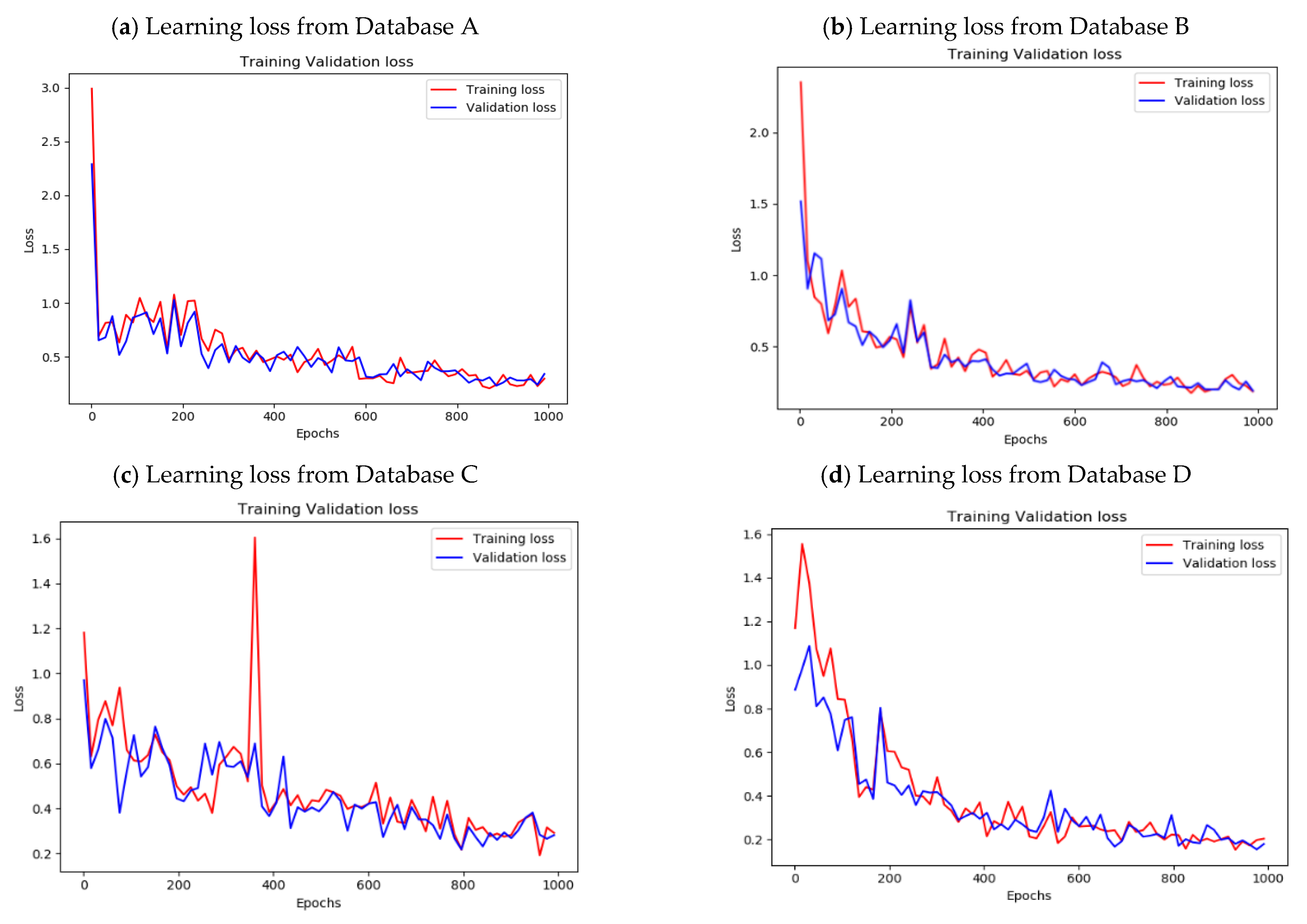
  • Database A, C: (Original database) 100 raw thermal images from thermal sequences with corresponding time;
  • Database B, D: (Mixed database) 100 raw thermal images with 100 new synthetic images; both selected from the same corresponding time;
All thermal images in the four training databases (A; B; C; and D) were preprocessed by the method in Section 3.3 in order to enhance the defect contrast.
Two raw (without preprocessing) thermal databases (E; F) (each consisting of 50 images) were used to validate the trained model (Mask-RCNN). These sequences, which have different shapes and depths of defects, were compared with the sequences during training. For sake of consistency, the raw thermal plexiglass database E was validated on the learning model trained on plexiglass (A, B), whilst the raw thermal CFRP database F was used to validate the learning model trained on CFRP (C, D). The defect labels and instance are shown in Figure 7, which includes the following shapes: circle, multilateral; square, rectangle; multi-angle of defect instances. LabelMe Image Annotator [27] was employed to label each defect region on the images; this allowed giving a simple and standard manual annotation for all of the images.

5. Experimental Results and Implantation Details

5.1. Evaluation Metrics (Average Precision (AP) and Probability of Detection (POD))

Average precision (AP) [28] is introduced to evaluate the performance capability of the detection model, which is analyzed by Equations (5) and (6).
P r e c i s i o n = T P T P + F P
  R e c a l l = T P T P + F N
where TP is the true positive rate. FP is the false positive rate, which indicated that defects are in the non-defects regions and are falsely detected as defects. FN is the false negative rate, representing a certain number of the defects that failed to be detected during this experiment. Precision represents the accuracy of the prediction from the performance of the model. Recall represents the performance of the model to find all the possible positive cases in top priorities predictions.
In this work, a definition of Probability of Detection (POD) [29] (Equation (7)) also has been introduced to measure how reliable the non-destructive texting automatic inspector will be for a given case. POD is a specific metric especially for characterizing and quantifying defect analysis in NDT methods.
P O D = T P T P + F N   ( C o n f i d e n c e   s c o r e = 0.75 )
The mathematical equation of POD keeps the same mathematical format as Recall in Equation (6), but they have different descriptions and explanations. In Equation (7) of POD, TP refers to true positive cases, which represent flaws in the system that the method can identify; FN refers to a false negative case, which indicates that the system has a flaw but the method cannot identify it. As a result, POD indicated how many flaws can truly be detected in a system from the whole amount of positive detected flaw cases.
In addition, we also introduced a definition herein for the further discussion of POD and defect classification-confidence score [30]. The confidence score can illustrate to which degree it is possible that the actual region boundaries overlap with the predicted defect region boundaries. In this work, our confidence score is set up as 0.75, which was selected as an acceptance criterion to define the percentage of the ground truth boundaries overlap with the predicted defect region boundaries for segmentation.
Therefore, the Probability of Detection (POD) assesses the performance of the Mask-RCNN (with synthetic data/without synthetic data) from the non-destructive evaluation-based inspection (NDE), which could determine the capability of the detection as a function of defect type. The probability of detection can form a core mathematical equation for examining and evaluating of the materials, which is also recognized as the quantitative evaluation tool involving the human factor and the various inspection parameters.

5.2. Main Results Analysis and Discussion

The operating system is set as Ubuntu 14.04; CPU: i7-5930k; Memory: 64GB. Each training processing was conducted on a GPU (NVIDIA GeForce GTX 1080Ti) and required approximately 30 min. Some main hyper-parameters and training parameters are set as below: (1) The Network training used Resnet101 as a backbone; (2) The learning momentum is 0.9 and learning rate is 0.0003; (3) The first 30 epochs were trained on network heads; then, all network layers were trained for 1030 epochs, the model weight (in h5 format) used was COCO (could be replaced with the original weight model file). This could be improved if a similar binary segmentation weight model was used; (4) The weight decay is 0.0001 and mini mask size is 56 × 56.

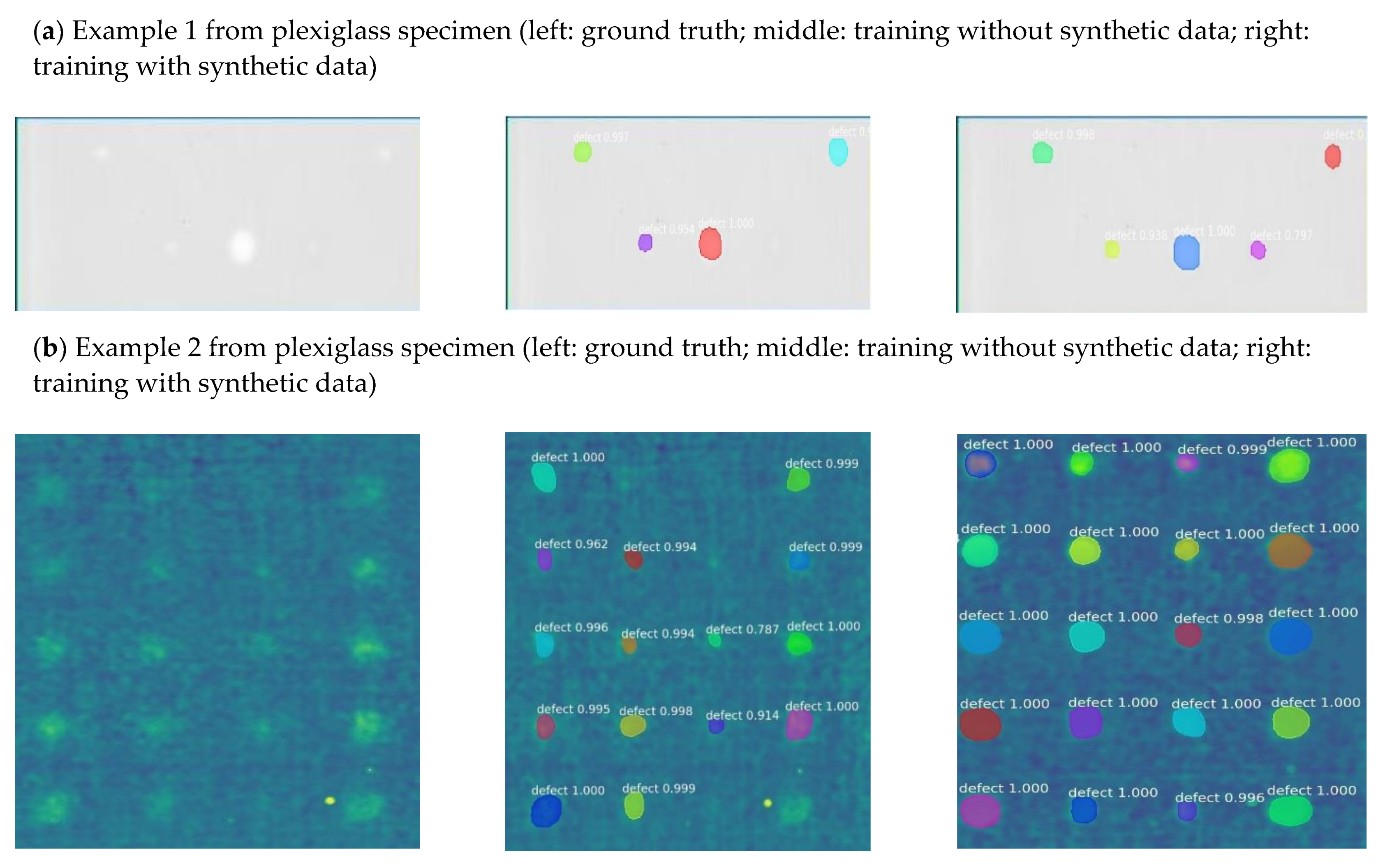
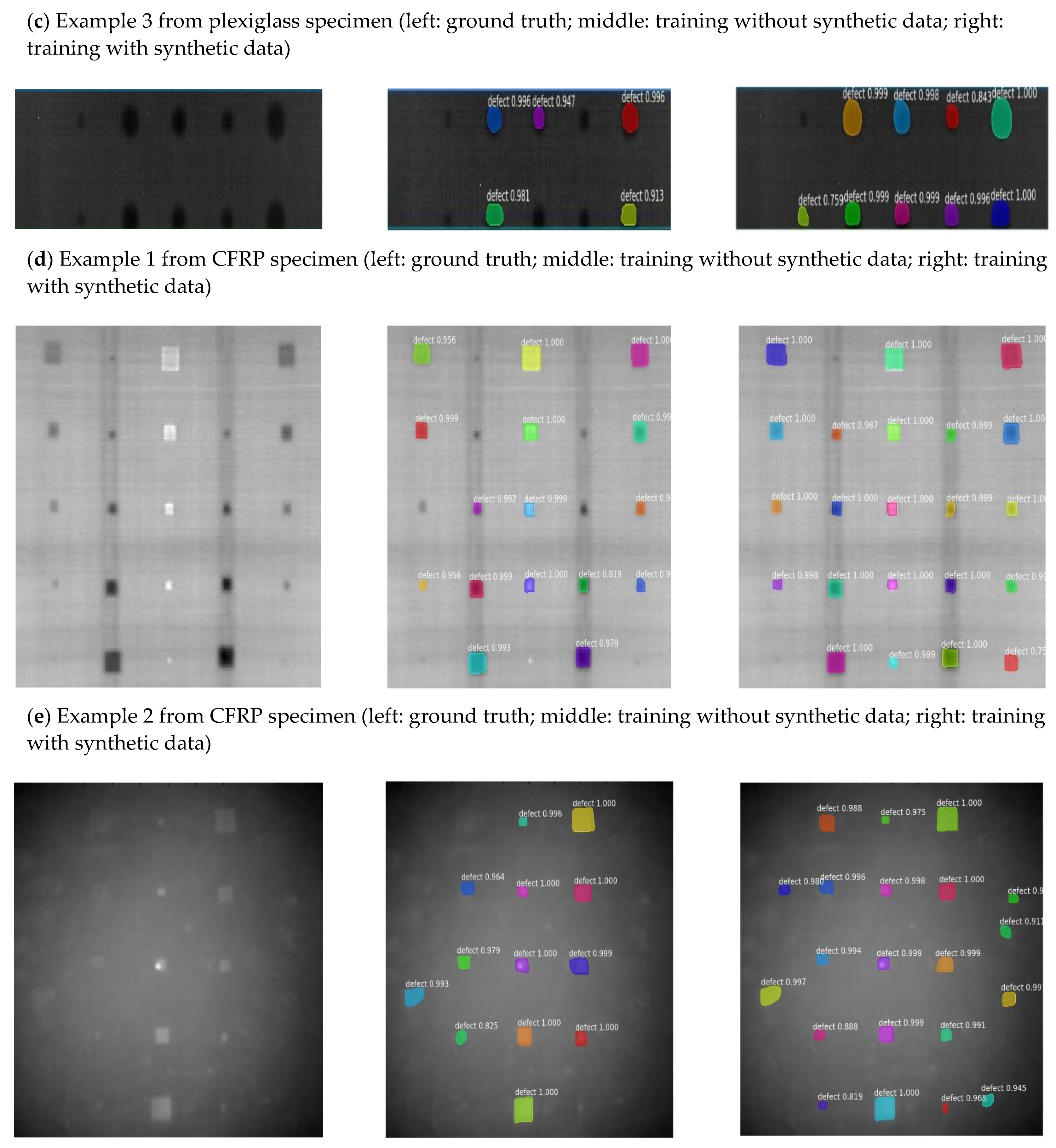
5.2.1. Segmentation Results and Learning Curves

As shown in Figure 8 below, the segmentation results of five examples Figure 8a–e from the Mask-RCNN model are indicated. The segmented results in the middle column were the validated results from the model trained on raw images after preprocessing (Database A, C). The segmented results in the right column were the validated results from the model trained on raw images merged with synthetic images after preprocessing (Database B, D). Meanwhile, in the first three rows, the results from plexiglass specimens (Validation Database E) are shown. The last two rows show the results for CFRP specimens (Validation Database F). The segmented defects from obtained images clearly show the improvement when trained on raw images merged with synthetic images after preprocessing in Figure 8. Although each segmented region has different color, all the colorful regions in the images represent true positive detective cases.
In addition, we can see the segmented results from the last column in Figure 8. When the model is trained with raw images (in the middle column), then the model is able to detect 12 defects out of 25 defects in the whole specimen with limited raw images during the validation. Each detected defect is covered by a solid mask. It is notable that the model produces one false positive defect case by highlighting one non-existing defect on the image and 13 false negative defects (less visible defects, which are difficult to detect). Further, in the right column, when the training of the databases was increased with synthetic data, the trained model is able to detect 17 defects in total. However, four false positive and false negative cases still appear on the image.
The learning loss indicated how well the learning model performed. In this experiment, Figure 9a,b showed the acquired average loss curve of the training and validation on Database A, B. The loss has a certain range of oscillation during the first 800 epochs in both Figure 9a,b; then, it decreases less rapidly after 800 epochs until it flattens out. The cost curve is decreasing as the batch number increases and converges approximately from 0.25. Correspondingly, Figure 9b,c indicate the learning curve with training and validation on Database C, D. The learning curve of the training and validation for Database D became more stable compared with the curves in Figure 9c. Although the validation loss from Figure 9c is instantly unstable around the point of the 380th epoch, the learning curves of training and validation (Database C, D) eventually converge around 0.2 around the 1000th epoch. Meanwhile, the model accuracy of the validation from Database A, B, C, D in this experiment is respectively 0.990, 0.996, 0.98738, and 0.98738. We obtained the model accuracy from four different training databases: B (0.996) > A (0.990) > C (0.987) = D (0.987). As a result, the obtained model accuracy from four groups of databases is impressive and shows the good performance during the training and validation when the Mask-RCNN model is used for defect segmentation of plexiglass and CFRP specimen in this project.

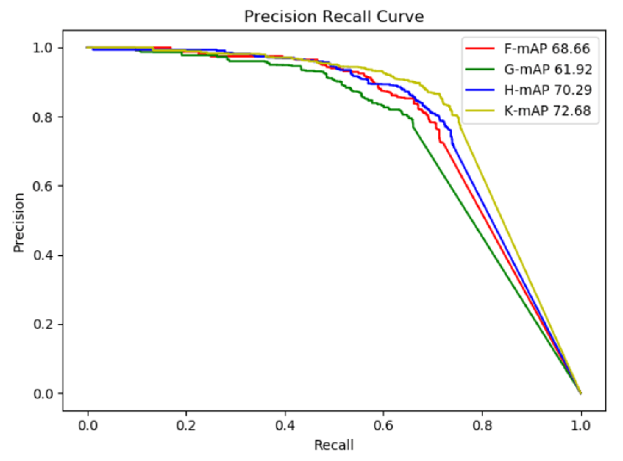
5.2.2. Precision–Recall Curves (PR Curves)

Precision–recall curves [31] for the Mask-RCNN architectures trained on four different groups of databases are shown in Figure 10. This figure indicated two PR curves for training sets of plexiglass specimens (preprocessed raw images database (A); synthetic images merging with raw images database from preprocessing (B)); an independent pure raw images validation set without preprocessing (E)) and two PR curves for training sets of CFRP specimens (preprocessing raw images database (C); synthetic images merging with raw images database from preprocessing (D); an independent pure raw images validation set without preprocessing (F)). The mean average precision (mAP) values in databases A, B, C, and D respectively reach 68.66, 76.40, 70.29, and 72.68 as shown in Figure 10.
During the training of Database (B, D), Mask-RCNN has seen limited preprocessed raw thermal images (100 images) merging with preprocessed synthetic data (beyond pretraining of the early layers on COCO [32]). The mAP values in the mixed database (B, D) are higher than those of Databases (A, C) (B (76.40) > A (68.66); D (72.68) > C (70.29)). From the plot of the PR curves, Database B achieves higher precision than Database A consistently for all of the recall values in the Mask-RCNN model. On the other hand, database D consistently obtained lower precision than database C between the recall values from 0.5 to 0.55. This helps explain that the plexiglass database obtained the higher mAP difference compared with CFRP between the training of raw images and the training from databases merging with synthetic data.
In each region of interest (ROI), this experiment obtained better results with the performance metric of precision and recall values compared with another cited deep learning IRT project [5,33]. Especially, the plexiglass obtained a superior performance of mAP from Mask-RCNN when it was merged with synthetic data for training compared with the highest mAP value obtained from previous research. This compelling performance also illustrates the ability of synthetic data to bridge the reality gap and demonstrates that merging with synthetic data for training can improve the accuracy in both types of material (CFRP; plexiglass). As a result, the training model merged with synthetic images could be able to outperform databases with pure raw thermal databases in deep learning IRT projects.

5.2.3. Evaluation with Probability of Detection

The Probability of Detection has been successfully applied for analyzing the detection capability of materials from Mask-RCNN. In this study, the POD was classified as a function of an aspect ratio r = diameter (D)/depth (d). Each POD point on the curve corresponds to a specific aspect ratio from a particular diameter (D) and depth (d). As indicated in Figure 11a, the red POD curve (Database B) maintained the highest POD curve from the whole aspect ratio, which indicated that the Mask-RCNN with synthetic data detected the largest percentage of defects in plexiglass specimens. Simultaneously, the POD of Database B is better than the corresponding POD curves (Database A), confirming that synthetic data merged with raw data can contribute to achieve better performance as compared to the model trained with raw data only. Based on these results, the POD of the databases that merged with synthetic data (B; C) has a better detection capability than any other database without synthetic data (A; D), revealing that merging the raw databases with synthetic data could be a reliable procedure for a deep learning model (Mask-RCNN), enhancing the capability of automatic defect segmentation and identification. The pink POD curve (C), which represents the CFRP database training with synthetic data, has an overall higher detection probability than the blue curve (D) (CFRP database training without synthetic data). However, in comparison with the POD curve (A; B), the POD curve (D) shows a lower detection performance than the POD curve A due to data diversity and data augmentation capability (different defect shapes and multiple angles, diverse formatted defects) that PLEXI databases have. As a result, PLEXI databases outperformed CFRP databases on the probability scores in this case.

5.2.4. Defect Classification Analyses

As indicated in Table 1 below, the detection with defects in each training database (A, B, C, D) by the Mask-RCNN algorithm in pulse thermography has been investigated with the objective to measure the global accuracy in each database [34]. Four confusion matrixes from training databases A, B, C, and D have been indicated, where TP = True Positive, FP = False Positive, TN = True Negative, and FN = False Negative. Each column of the matrix stands for the objectives in the actual class; simultaneously, each row of the matrix stands for the objectives in the predicted class.
The results from detection have shown an excellent performance when the original database was merged with synthetic data based on the number of well-classified labels. The approximately average prediction of each database is shown in the Table 1. We set up the confidence score threshold as 75% of probability of detection to distinguish TP, FP, TN, and FN cases.
As mentioned earlier, the objective in this research is to automatically extract and segment the features (i.e., defects) that could be found in each thermal frame. Each classification may either be a defect or a non-defect region in this task. In data science, an effective metric to validate the performance of a detection algorithm widely used in the deep learning applications is the confusion matrix [35]. In the confusion matrix, each matrix is set up 2 × 2, where 2 is the number of classes in the dataset. The row elements of a confusion matrix represent the classes to which the features of the image belong, either to the feature region of a defect or a non-defect. Its columns, on the other hand, represent the classes given by the Mask-RCNN during the segmentation process.
Generally, in this case, based on Table 1 (confidence score = 75%), the testing Database E with the training Database A, 1785 defects were segmented correctly, 456 were missed, 229 non-defect regions were detected as defects, and 291 non-defect regions were correctly labeled as non-defects in this experiment. In the case of testing Database E with the training Database B, 2060 defects were detected correctly, 182 were missed, 199 non-defect regions were detected as defects, and 321 non-defect regions were correctly labeled as non-defect in this experiment. In the case of the testing Database F with the training Database C, 1442 defects were detected correctly, 358 were missed, 257 non-defect regions were detected as defects, and 296 non-defect regions were correctly labeled as non-defect in this experiment. In the case of the testing Database F with the training Database D, 1610 defects were detected correctly, 190 were missed, 225 non-defect regions were detected as defects, and 328 non-defect regions were correctly labeled as non-defects in this experiment. Then, it can be concluded from the confusion matrix that after merging with synthetic data, Mask-RCNN leads to a superior performance in defects detection than the results obtained previously.
In addition, the global accuracy Acc given in the corresponding training databases (A–D) and test databases (E, F) in Figure 12 is defined in Equation (8). The implementation of the deep leaning model (Mask-RCNN) used for the whole validation process is set according to the principle as follows: the specific testing Dataset (E) corresponding to the training data (A, B); the specific testing data (F) corresponding to the training data (C, D) respectively.
  A c c = A v e r a g e   t o t a l   a c c u r a c y = c o r r e c t l y   c l a s s i f y   r e g i o n s T o t a l   n u m b e r   o f   e v l u a t e d   r e g i o n s    

5.2.5. The Comparisons with State-of-the-Art Deep Learning Detection Algorithms

In this session, YOLO-V3 and Faster-RCNN have been selected as the state-of-the-art object detectors to compare with the performance of Mask-RCNN when it is merged with the synthetic data or without during the training. A CFRP specimen has to be validated on four different training situations from Database C, D in Section 4 for three types of object detectors in Figure 13, which included (a) Mask-RCNN training with Database C; (b) Mask-RCNN training with Database D; (c) YOLO-V3 training with Database C; and (d) Faster-RCNN training with Database C.
It can be seen from the Figure 13 that when Mask-RCNN was only training with experimental data in Figure 13a, it obtained similar accuracy based on comparing the results those of with YOLO-v3 in Figure 13c and Faster-RCNN in Figure 13d. However, after the training databases merged with synthetic data in Figure 13b, the results from Mask-RCNN outperformed the other three different situations.
On the other hand, frames per second (fps) [36] has been introduced as a concept to verify how many pictures can be processed in a unit time (one second) by an objective detector in order to evaluate the running time complexity for each detector. In Table 2, the time complexity of three deep learning algorithms have been illustrated. In this experiment, during the training processing being conducted on GPU (NVIDIA GeForce GTX 1080Ti YOLO-V3, three deep learning detectors YOLO-V3, Mask-RCNN, Faster-RCNN running are 15 fps, 5fps, and 1fps, respectively. As a result, comparing with Mask-RCNN and Faster-RCNN, YOLO-V3 has the highest running time speed to process images due to the reason that YOLO-v3 is a one-stage real-time detector, and it has a much faster speed than other detectors (Mask-RCNN; Faster-RCNN), which are two-stage procedures (Region Proposal Network (RPN); ROI pooling). However, as indicated in Figure 14, Mask-RCNN still obtained higher POD scores during the whole validation process when it merged with synthetic data based on the different ratio values (size/depth).

6. Result Analysis and Discussion

The main objective of synthetic data in this project is to enlarge the datasets when you only have limited raw experimental data. Synthetic data can more easily generate a dataset with a large amount of variety. Small raw training databases merging with synthetic data can help detect most of the defects successfully while avoiding expensive experiments. As we can see from Section 5.2.2, Figure 10, which shows the performance of the definite and regularly used evaluation metric (precision and recall), higher average precision gives better results when trained on the data merging with synthetic data than when trained on the raw data only. Therefore, we are able to boost the model performance by feeding the synthetic data to merge or replace the actual one.
This confirmed that in different situations, when the synthetic data merged with the sample, it can actually benefit the learning network, enabling it to learn and understand the pattern by (a) generating more significant samples than the original available data, which is limited; (b) providing more data of any specific minority cases (for example, the highly expensive thermal data of the CFRP samples, which is difficult to obtain) in order to avoid the underrepresentation or underperformance situation for automatic defects segmentation.
Comparing with the up-to-date CNN defect detection work [4,5,6,7,8] in infrared thermography as mentioned in introduction, the Mask-RCNN model merging with synthetical data has become the most flexible method that has the capacity to obtain the improvable performance. Especially in pulsed thermography, too little data might be available and obtained in the realistic experiment. It is always too expensive and time-consuming to training with the additional thermal data during the training and defect detection by the deep learning algorithm. Therefore, the generated synthetic data show their ability to support this case. As indicated in Figure 11 of Section 5.2.3, the POD curve of Database D exceeds the POD curve of Database C from all aspect ratio values (size/depth), which illustrated that synthetic data have the potential to immensely improve performance in regard to defect detection for CFRP and plexiglass specimens. On the other hand, in the defect classification analysis in Figure 12 from Section 5.2.4, the global accuracy Acc increasing predominately from the testing results when the trained system performed with Database B and Database D, which further demonstrated that a trained system merged with synthetic data may beneficial for detecting and identifying defects.
As shown in the results from different objective detectors indicated by the POD evaluations from Figure 14 (Section 5.2.5), it is obvious that YOLO-V3 obtained comparable accuracy with the Mask-RCNN method during the whole validation process, while the Faster-RCNN gave mediocre performance. However, after merging with synthetic data, our proposed method shows excellent performance because the data augmentation strategy has a strong effect on the capability of the Mask-RCNN model to capture less visible defects and separate low-rank non-defect information from the thermal data, after which the meaningful features remain. It is worth mentioning that the proposed method (Mask-RCNN) maintains the highest accuracy in POD evaluation when it encounters the challenging and lowest (0–5) aspect ratio value (size/depth). With all task-driven objective detectors based on the deep learning architecture, the proposed method keeps the highest accuracy results over the other state-of-the-art algorithms. This excellent performance is thanks to the capability of the synthetic data generation pipeline’s data augmentation strategy to segment the defects from the multi feature distribution.
Furthermore, as mentioned in Section 3.2, the COMSOL is capable of creating high-quality synthetic thermal data from scratch on specific data points and the same heat transfer principles setting from pulsed thermography. However, based on the results, there is still some room for improvement. The defects from synthetic data (COMSOL) may still have blurry boundaries and unclear shapes that influence the training results from learning. Mask-R-CNN is robust to the limited size of synthetic data and is more likely to overfit unless the data increase the augmentation (rotating, flipping images, or random Gaussian noise). We applied the following data augmentation strategy: flip, rotation, scale, crop and adding the Gaussian noise to each individual synthetic and raw image. We stopped all the training during the time of the performance, nearly saturating with the overfitting.
In additional, in this task, we used Resnet101 [37] as a feature extractor with weights initialized from COCO in Mask-RCNN. Since the weights from COCO obtained the features trained by a group of datasets that contain basic lines and shapes of the objectives (circle, square, rectangle), it can be beneficial to the defect detection to a certain degree even without training with thermal images. So, the selection of beneficial initial weights from the pretrained models could be a key training strategy to apply for the future direction of research in deep learning IRT.
In future work, the other available thermography methods in the literature will be implemented with Mask-RCNN and a synthetic data generation pipeline to further exploit its possibility to enhance its capability of defect detection. A modified version of the Mask-RCNNN network will be introduced for enhancing its training performance. The further plan can be also illustrated as follows: (a) enhancing the training performance by adjusting the key parameters and structure in Mask-RCNN; (b) exploitation of variety software in Finite Element Modeling for generating synthetical data for defect detections for comparison with COMSOL; (c) Mask-RCNN with a synthetic data generation pipeline test with other NDT techniques to evaluate the performance of defect analysis.

7. Conclusions

In summary, we present a method where the deep learning architecture is combined with a small amount of synthetic thermal data for defect segmentation. The proposed architecture is based on a Mask-RCNN that has been applied in natural image segmentation. We collected our thermal database from the experimental results and synthetic data in the Finite Element Model (COMSOL). The network yields a better performance when it is fused with synthetic data for training. Meanwhile, different types of composite materials (CFRP; plexiglass) with defects have been validated via the proposed method to reveal the performance of detection. The proposed algorithm, Mask-RCNN without modification, is in line with the main objective in this work, which is to assess whether synthetic data can improve the detection accuracy of defects on the CFRP or plexiglass composite samples. Further quantitative analysis of the diameter/depth ratio with POD evaluation in defect detection with a modified structured Mask-RCNN network will be carried out in future work.

Author Contributions

Conceptualization, Q.F. and X.M.; methodology, Q.F.; software, Q.F.; validation, Q.F., C.I.-C. and X.M.; formal analysis, C.I.-C.; investigation, Q.F.; resources, X.M.; data curation, Q.F.; writing—original draft preparation, Q.F.; writing—review and editing, Q.F., C.I.-C.; visualization, Q.F.; supervision, X.M., C.I.-C.; project administration, X.M. C.I.-C.; funding acquisition, X.M. All authors have read and agreed to the published version of the manuscript.

Funding

This research received funding support from NSERC DG program, the Canada Foundation for Innovation and the Canada Research Chair program. We want also to acknowledge the financial support and help of the Chinese Scholarship Council.

Institutional Review Board Statement

No institutional board review was necessary for this project.

Informed Consent Statement

Informed consent was obtained from all subjects involved in the study.

Data Availability Statement

Data available on request from the authors.

Acknowledgments

This research is conducted under the Tier One-Multipolar Infrared Vision Canada Research Chair (MIVIM) in the Department of Electrical and Computer Engineering at Laval University. The authors would like also specially thank the contributions from Farima. Abdolahi. Mamoudan (MIVIM group, Universite Laval) for the COMSOL simulation, experimental session in this article.

Conflicts of Interest

The authors declare no conflict of interest.

References

  1. Ferguson, M.K.; Ronay, A.; Lee, Y.T.T.; Law, K.H. Detection and Segmentation of Manufacturing Defects with Convolutional Neural Networks and Transfer Learning. Smart Sustain. Manuf. Syst. 2018, 2. [Google Scholar] [CrossRef] [PubMed]
  2. Maldague, X.; Krapez, J.C.; Poussart, D. Thermographic nondestructive evaluation (NDE): An algorithm for automatic defect extraction in infrared images. IEEE Trans. Syst. Man Cybern. 1990, 20, 722–725. [Google Scholar] [CrossRef]
  3. Rajic, N. Principal Component Thermograph; Defence Science and Technology Organisation Victoria (Australia) Aeronautical and Maritime Research Lab: Fisherman’s Bend, VIC, Australia, 2002. [Google Scholar]
  4. Hu, J.; Xu, W.; Gao, B.; Tian, G.Y.; Wang, Y.Z.; Wu, Y.C.; Yin, Y.; Chen, J. Pattern deep region learning for crack detection in thermography diagnosis system. Metals 2018, 8, 612. [Google Scholar] [CrossRef] [Green Version]
  5. Fang, Q.; Nguyen, B.D.; Castanedo, C.I.; Duan, Y.X.; Xavier, M. Automatic Defect Detection in Infrared Thermography by Deep Learning Algorithm. Available online: https://www.spiedigitallibrary.org/conference-proceedings-of-spie/11409/2555553/Defects-detection-in-infrared-thermography-by-deep-learning-algorithm/10.1117/12.2555553.short?SSO=1 (accessed on 26 February 2021).
  6. Jia, F.; Lei, Y.; Guo, L.; Lin, J.; Xing, S. A neural network constructed by deep learning technique and its application to intelligent fault diagnosis of machines. Neurocomputing 2018, 272, 619–628. [Google Scholar] [CrossRef]
  7. Janssens, O.; Van de Walle, R.; Loccufier, M.; Van Hoecke, S. Deep learning for infrared thermal image based machine health monitoring. IEEE/ASME Trans. Mechatron. 2017, 23, 151–159. [Google Scholar] [CrossRef] [Green Version]
  8. Zhang, Y.; Fjeld, M. Condition Monitoring for Confined Industrial Process Based on Infrared Images by Using Deep Neural Network and Variants. Available online: https://www.researchgate.net/publication/340599990_Condition_Monitoring_for_Confined_Industrial_Process_Based_on_Infrared_Images_by_Using_Deep_Neural_Network_and_Variants (accessed on 26 February 2021).
  9. Torrey, L.; Shavlik, J. Transfer learning. In Handbook of Research on Machine Learning Applications and Trends: Algorithms, Methods, and Techniques; IGI global: Hershey, PA, USA, 2010; pp. 242–264. [Google Scholar]
  10. He, K.; Gkioxari, G.; Dollár, P.; Girshick, R. Mask r-cnn. In Proceedings of the IEEE International Conference on Computer Vision, Venice, Italy, 22–29 October 2017; pp. 2961–2969. [Google Scholar] [CrossRef]
  11. Ren, S.; He, K.; Girshick, R.; Sun, J. Faster r-cnn: Towards real-time object detection with region proposal networks. In Proceedings of the Advances in Neural Information Processing Systems, Montreal, Canada, 7–12 December 2015; pp. 91–99. [Google Scholar] [CrossRef] [Green Version]
  12. Long, J.; Shelhamer, E.; Darrell, T. Fully convolutional networks for semantic segmentation. In Proceedings of the IEEE Conference on Computer Vision and Pattern Recognition, Boston, MA, USA, 7–12 June 2015; pp. 3431–3440. [Google Scholar] [CrossRef] [Green Version]
  13. Ronneberger, O.; Fischer, P.; Brox, T. U-net: Convolutional networks for biomedical image segmentation. In Proceedings of the International Conference on Medical Image Computing and Computer-Assisted Intervention, Munich, Germany, 5–9 October 2015; Springer: Cham, Switzerland, 2015; pp. 234–241. [Google Scholar]
  14. Badrinarayanan, V.; Handa, A.; Cipolla, R. Segnet: A deep convolutional encoder-decoder architecture for robust semantic pixel-wise labelling. arXiv 2015, arXiv:1505.07293. [Google Scholar]
  15. Ren, M.; Zemel, R.S. End-to-end instance segmentation with recurrent attention. In Proceedings of the IEEE Conference on Computer Vision and Pattern Recognition, Honolulu, HI, USA, 21–26 July 2017; pp. 6656–6664. [Google Scholar]
  16. Tremblay, J.; Prakash, A.; Acuna, D.; Brophy, M.; Jampani, V.; Anil, C.; To, T.; Cameracci, E.; Boochoon, S.; Birchfield, S. Training deep networks with synthetic data: Bridging the reality gap by domain randomization. In Proceedings of the IEEE Conference on Computer Vision and Pattern Recognition Workshops, Salt Lake City, Utah, USA, 23 April 2018; pp. 969–977. [Google Scholar] [CrossRef] [Green Version]
  17. Richter, S.R.; Vineet, V.; Roth, S.; Koltun, V. Playing for data: Ground truth from computer games. In Proceedings of the European Conference on Computer Vision, Amsterdam, the Netherlands, 8–16 October 2016; Springer: Cham, Switzerland, 2016; pp. 102–118. [Google Scholar]
  18. McCormac, J.; Handa, A.; Leutenegger, S.; Davison, A.J. SceneNet RGB-D: 5M photorealistic images of synthetic indoor trajectories with ground truth. arXiv 2016, arXiv:1612.05079. [Google Scholar]
  19. Ibarra-Castanedo, C.; Maldague, X.P.V. Infrared Thermography. In Handbook of Technical Diagnostics; Springer: Berlin/Heidelberg, Germany, 2013; p. 826. [Google Scholar]
  20. Maldague, X. Theory and Practice of Infrared Technology for Non Destructive Testing; Wiley: New York, NY, USA, 2001; p. 684. [Google Scholar]
  21. Girshick, R. Fast r-cnn. In Proceedings of the IEEE International Conference on Computer Vision, Santiago, Chile, 7–13 December 2015; pp. 1440–1448. [Google Scholar] [CrossRef]
  22. Garcia-Garcia, A.; Orts-Escolano, S.; Oprea, S.; Villena-Martinez, V.; Garcia-Rodriguez, J. A review on deep learning techniques applied to semantic segmentation. arXiv 2017, arXiv:1704.06857. [Google Scholar]
  23. Kononenko, O.; Kononenko, I. Machine Learning and Finite Element Method for Physical Systems Modeling. arXiv 2018, arXiv:1801.07337. [Google Scholar]
  24. Beskos, D.E. Boundary element methods in dynamic analysis. Appl. Mech. Rev. 1987. [Google Scholar] [CrossRef]
  25. Chen, Z.; Xu, Y.; Zhang, Y. A construction of higher-order finite volume methods. Math. Comput. 2015, 84, 599–628. [Google Scholar] [CrossRef]
  26. Garrido, I.; Lagüela, S.; Sfarra, S.; Arias, P. Development of Thermal Principles for the Automation of the Thermographic Monitoring of Cultural Heritage. Sensors 2020, 20, 3392. [Google Scholar] [CrossRef] [PubMed]
  27. Russell, B.C.; Torralba, A.; Murphy, K.P.; Freeman, W.T. LabelMe: A database and web-based tool for image annotation. Int. J. Comput. Vis. 2008, 77, 157–173. [Google Scholar] [CrossRef]
  28. Robertson, S. A new interpretation of average precision. In Proceedings of the 31st Annual International ACM SIGIR Conference on Research and Development in Information Retrieval, Singapore, 20–24 July 2008; pp. 689–690. [Google Scholar] [CrossRef]
  29. Ahmad, J.; Akula, A.; Mulaveesala, R.; Sardana, H.K. Probability of Detecting the Deep Defects in Steel Sample using Frequency Modulated Independent Component Thermography. IEEE Sens. J. 2020. [Google Scholar] [CrossRef]
  30. Rezatofighi, H.; Tsoi, N.; Gwak, J.Y.; Sadeghian, A.; Reid, I.; Savarese, S. Generalized intersection over union: A metric and a loss for bounding box regression. In Proceedings of the IEEE Conference on Computer Vision and Pattern Recognition, Long beach, LA, USA, 16–20 June 2019; pp. 658–666. [Google Scholar] [CrossRef] [Green Version]
  31. Henderson, P.; Ferrari, V. End-to-end training of object class detectors for mean average precision. In Proceedings of the Asian Conference on Computer Vision, Taipei, Taiwan, 20–24 November 2016; Springer: Cham, Switzerland, 2016; pp. 198–213. [Google Scholar]
  32. Lin, T.Y.; Maire, M.; Belongie, S.; Bourdev, L.; Girshick, R.; Hays, J.; Perona, P.; Ramanan, D.; Zitnick, C.L.; Dollár, P. Microsoft coco: Common objects in context. In Proceedings of the European Conference on Computer Vision, Zurich, Switzerland, 6–12 September 2014; Springer: Cham, Switzerland, 2014; pp. 740–755. [Google Scholar]
  33. Manzano, C.; Ngo, A.C.Y.; Sivaraja, V.K.S.O. Intelligent Infrared Thermography Inspection of Subsurface Defects. Available online: https://www.spiedigitallibrary.org/conference-proceedings-of-spie/11409/114090V/Intelligent-infrared-thermography-inspection-of-subsurface-defects/10.1117/12.2558958.short (accessed on 26 February 2021).
  34. Hossin, M.; Sulaiman, M.N. A review on evaluation metrics for data classification evaluations. Int. J. Data Min. Knowl. Manag. Process 2015, 5, 1. [Google Scholar]
  35. Deng, X.; Liu, Q.; Deng, Y.; Mahadevan, S. An improved method to construct basic probability assignment based on the confusion matrix for classification problem. Inf. Sci. 2016, 340, 250–261. [Google Scholar] [CrossRef]
  36. Benenson, R.; Mathias, M.; Timofte, R.; Van Gool, L. Pedestrian detection at 100 frames per second. In Proceedings of the 2012 IEEE Conference on Computer Vision and Pattern Recognition, Providence, RI, USA, 16–21 June 2012; IEEE: New York, NY, USA, 2012; pp. 2903–2910. [Google Scholar] [CrossRef]
  37. Sitaram, S.; Dessai, A. Classification of Cervical MR Images Using ResNet101. Available online: https://www.ijresm.com/Vol.2_2019/Vol2_Iss6_June19/IJRESM_V2_I6_69.pdf (accessed on 26 February 2021).
Figure 1. Pulsed thermography experimental setup optical excitation.
Bdcc 05 00009 g001
Figure 2. Proposed segmentation strategy.
Bdcc 05 00009 g002
Figure 3. Mask-RCNN processing architecture [6].
Bdcc 05 00009 g003
Figure 4. (a) Finite Element Modeling (FEM) 3D model; (b) Simulated thermogram at t = 106.5 s; (c) Real experimental data t = 106.5 s.
Bdcc 05 00009 g004
Figure 5. Proposed workflow to train with a deep learning model based on the data generation by Finite Element Modeling.
Bdcc 05 00009 g005
Figure 6. Scheme of preprocessing stage.
Bdcc 05 00009 g006
Figure 7. Labels for preprocessed sample image.
Bdcc 05 00009 g007aBdcc 05 00009 g007b
Figure 8. The best obtained validation results of Mask-RCNN segmentation on different training databases. From left to right: original images, training on the preprocessed raw images database, training on the mixed database (preprocessed data from synthetic and raw images). From the first three rows to the last two rows: plexiglass (ac), carbon fiber-reinforced polymer (CFRP) (d,e).
Bdcc 05 00009 g008aBdcc 05 00009 g008b
Figure 9. The average learning loss for two types of specimens: plexiglass (a,b); CFRP (c,d).
Bdcc 05 00009 g009
Figure 10. Different detection results with four groups of datasets (two types of materials).
Bdcc 05 00009 g010
Figure 11. Probability of distribution curve of different methods for processing on CFRP samples (a)/PLEXI samples (b) (confidence score = 0.75).
Bdcc 05 00009 g011
Figure 12. The total performance of accuracy with Mask-RCNN on CFRP and PLEXI samples with/without synthetic data.
Bdcc 05 00009 g012
Figure 13. Detection results on a reprehensive CFRP specimen provided by different objective detection algorithms or scenarios (a) Master-RCNN without synthetic data; (b) Master-RCNN with synthetic data; (c)YOLO-V3; (d) Faster-RCNN.
Bdcc 05 00009 g013
Figure 14. Probability of distribution of different deep learning methods on CFRP databases (confidence score = 0.75).
Bdcc 05 00009 g014
Table 1. Class mark list—comprehensive results.
DatabaseA/E *B/E *
Actual Class
ClassDefectNon-defectDefectNon-defect
PredictedDefectTP: 1785FP: 229TP: 2060FP: 199
ClassNon-defectFN: 456TN: 291FN: 181TN: 321
DatabaseC/F *D/F *
Actual Class
ClassDefectNon-defectDefectNon-defect
PredictedDefectTP:1442FP: 257TP: 1610FP: 225
ClassNon-defectFN: 358TN: 296FN: 190TN: 328
* Training database/Testing database.
Table 2. Running time complexity comparison with state-of-the-art methods.
Running Time ComplexityYOLO-V3Mask-RCNNFaster-RCNN
Frame per second (FPS)1551
Publisher’s Note: MDPI stays neutral with regard to jurisdictional claims in published maps and institutional affiliations.

