
Estimating Causal Effects When the Treatment Affects All Subjects Simultaneously: An Application


Department of Economics, Management and Statistics (DEMS), University of Milano-Bicocca, 20126 Milan, Italy
Big Data Cogn. Comput. 2021, 5(2), 22; https://0-doi-org.brum.beds.ac.uk/10.3390/bdcc5020022
Submission received: 18 March 2021
/
Revised: 26 April 2021
/
Accepted: 29 April 2021
/
Published: 6 May 2021
(This article belongs to the Special Issue Big Data Analytics for Social Services)
Abstract
:Several important questions cannot be answered with the standard toolkit of causal inference since all subjects are treated for a given period and thus there is no control group. One example of this type of questions is the impact of carbon dioxide emissions on global warming. In this paper, we address this question using a machine learning method, which allows estimating causal impacts in settings when a randomized experiment is not feasible. We discuss the conditions under which this method can identify a causal impact, and we find that carbon dioxide emissions are responsible for an increase in average global temperature of about 0.3 degrees Celsius between 1961 and 2011. We offer two main contributions. First, we provide one additional application of Machine Learning to answer causal questions of policy relevance. Second, by applying a methodology that relies on few directly testable assumptions and is easy to replicate, we provide robust evidence of the man-made nature of global warming, which could reduce incentives to turn to biased sources of information that fuels climate change skepticism.
1. Introduction
An emerging literature has discussed the contributions of Machine Learning (ML) to address relevant policy questions [1,2,3,4,5]. One important contribution is the development of better prediction methods [6,7] to answer causal questions that involve prediction [1,8] when a treatment affects all subjects simultaneously [9]. In such a context, all subjects are treated for a given period, and thus there is no control group, so that a randomized control trial is not viable and the standard quantitative toolkit of causal inference cannot be used.
One example of this type of questions is the impact of anthropogenic emissions on global warming. In an ideal experiment designed to measure this effect, we would take two identical populations and expose one to a control level of anthropogenic emissions and the other one to a treatment level of emissions. The control population would serve as the counterfactual, and the difference in temperature between the treatment and the control population would measure the effect of the anthropogenic emissions on temperature. However, this experiment is not feasible since all populations are exposed to and affected by emissions simultaneously.
To address the problem of the missing counterfactual, an extensive literature has used a variety of econometrics methods and has built a scientific consensus on the man-made nature of global warming [10,11]. However, climate change denial is still present. The literature on climate change perceptions attributes this in part to the complexity of the techniques involved in the analysis of climate data, which incentivizes individuals to defer to the often biased information on climate change that political parties provide [12].
Recent advancements in ML provide simple and easily replicable methods to predict the missing counterfactual. One of these methods is the Bayesian Structural Time Series (BSTS) estimator developed by the authors of [13]. Given a response time series and several control series, the method consists in estimating a BSTS model using the data before the treatment takes place to predict the counterfactual, that is, what would have happened absent the treatment in the post-treatment period. The method relies on a few directly testable assumptions that facilitate results’ interpretation and replicability.
We apply the BSTS estimator to estimate the causal effect of anthropogenic emissions on global warming using yearly data on global temperature and all sources of natural and anthropogenic emissions between 1850 and 2011. We define as treatment the increase in CO emissions in 1960, and we estimate a BSTS model to assess the impact of CO emissions as the external factor that could have caused the post-1960 increase in global temperature. We find that the increase in CO emissions contributed to a temperature increase of 0.3 degrees Celsius between 1960 and 2011. This is a substantial increase, which is consistent with the findings of the previous literature [10]. Using a methodology that is directly replicable and relies on a few testable assumptions, this paper provides robust evidence that strengthens the consensus on the impact of human activities on global warming and the urgency to take action to limit emissions.
We make two main contributions: first, we draw attention to an ML method that can be successfully used to estimate causal impacts in settings when a randomized experiment is not viable; in doing so, we contribute to the emerging field that merges social sciences and ML to answer causal questions of policy relevance [1,2,4,5,9,14]. Second, by applying a methodology that relies on a few directly testable assumptions and is easy to replicate, we provide robust evidence of the man-made nature of global warming, which could be used to communicate results and reduce people’s incentives to turn to biased sources of information that fuel climate change skepticism.
The remainder of the paper is organized as follows. Section 2 describes the data. Section 3 presents the model. Section 4 discusses the model’s estimation and Section 5 discusses validity and identification. Section 6 presents the main empirical results and the robustness checks. Section 7 discusses the results and briefly concludes.
2. Data
In order to study the impact of anthropogenic emissions on global warming, we need data on changes in global temperature and on all the factors affecting these changes. In the literature, changes in global temperature are measured using temperature anomalies, which are deviations of the average global temperature with reference to a baseline period, typically defined as the long-term average between 1961 and 1990, and changes in temperature anomalies depend on radiative forcing (RF) due to natural and human activities. RF quantifies the changes in energy flows due to natural phenomena (natural RF) or human activities (anthropogenic RF). Anthropogenic RF includes greenhouse gases, sulfur emissions, and black and organic carbon, whereas natural RF is due to volcanic eruptions and solar activity. Greenhouse gas emissions include emissions of carbon dioxide (CO), methane, dinitrogen oxide, and chlorofluorocarbons (CFC11 and CFC12).
The authors of [15] compiled a comprehensive dataset with annual records on global temperature anomalies from two different sources (the HaDCRUT4 and the GISS v3 datasets), ocean heat content, and all sources of RF for each year between 1850 and 2011.
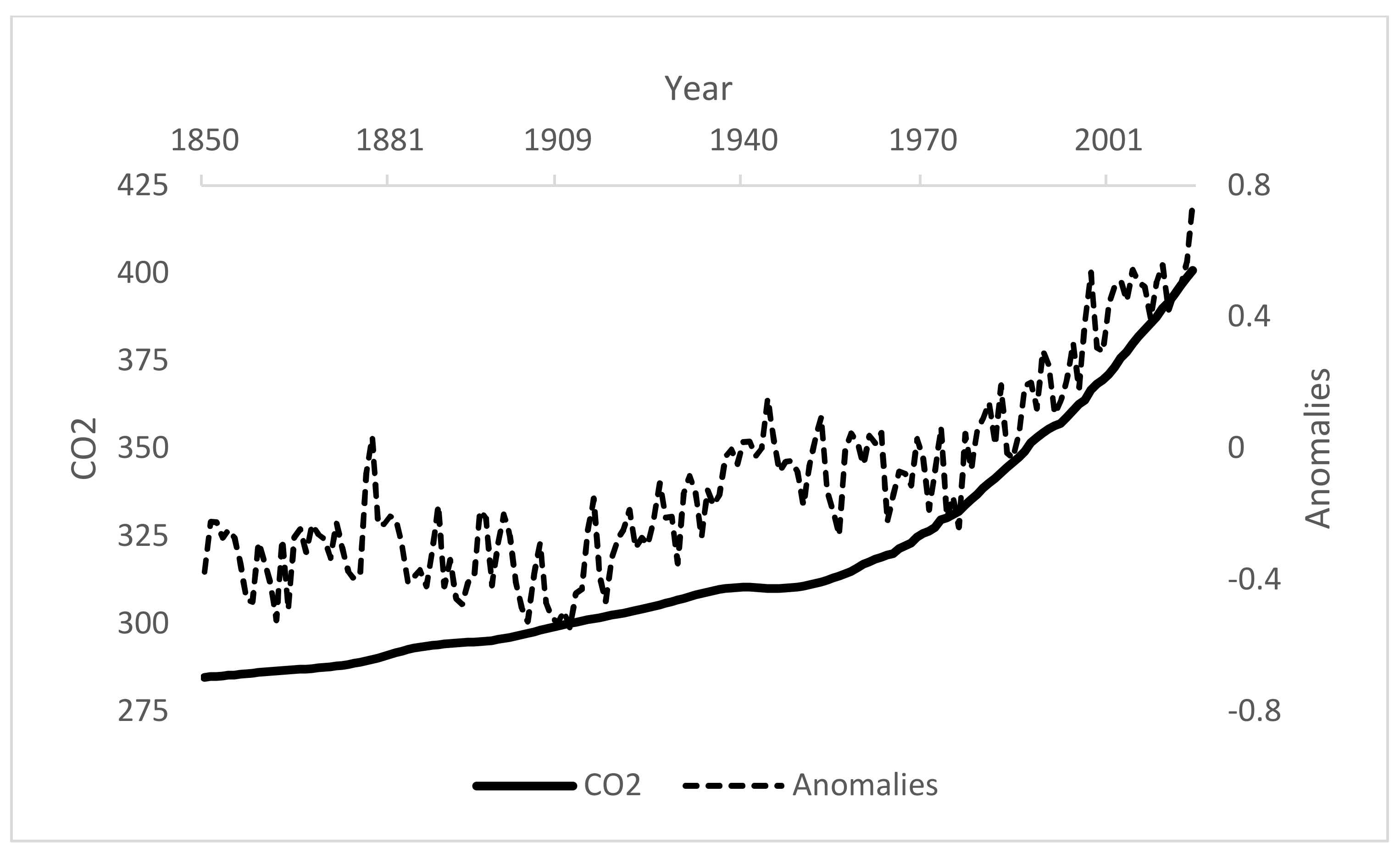
Figure 1 presents yearly records of atmospheric concentration levels of CO emissions (bold line) and temperature anomalies (dashed line) using the HadCRUT4 temperature data, and shows a strong correlation between temperature anomalies and CO emissions since the year 1960. As documented by the previous literature [16], CO emissions started increasing in 1960, and increased even more, at a yearly rate of , between 1975 and 2005.
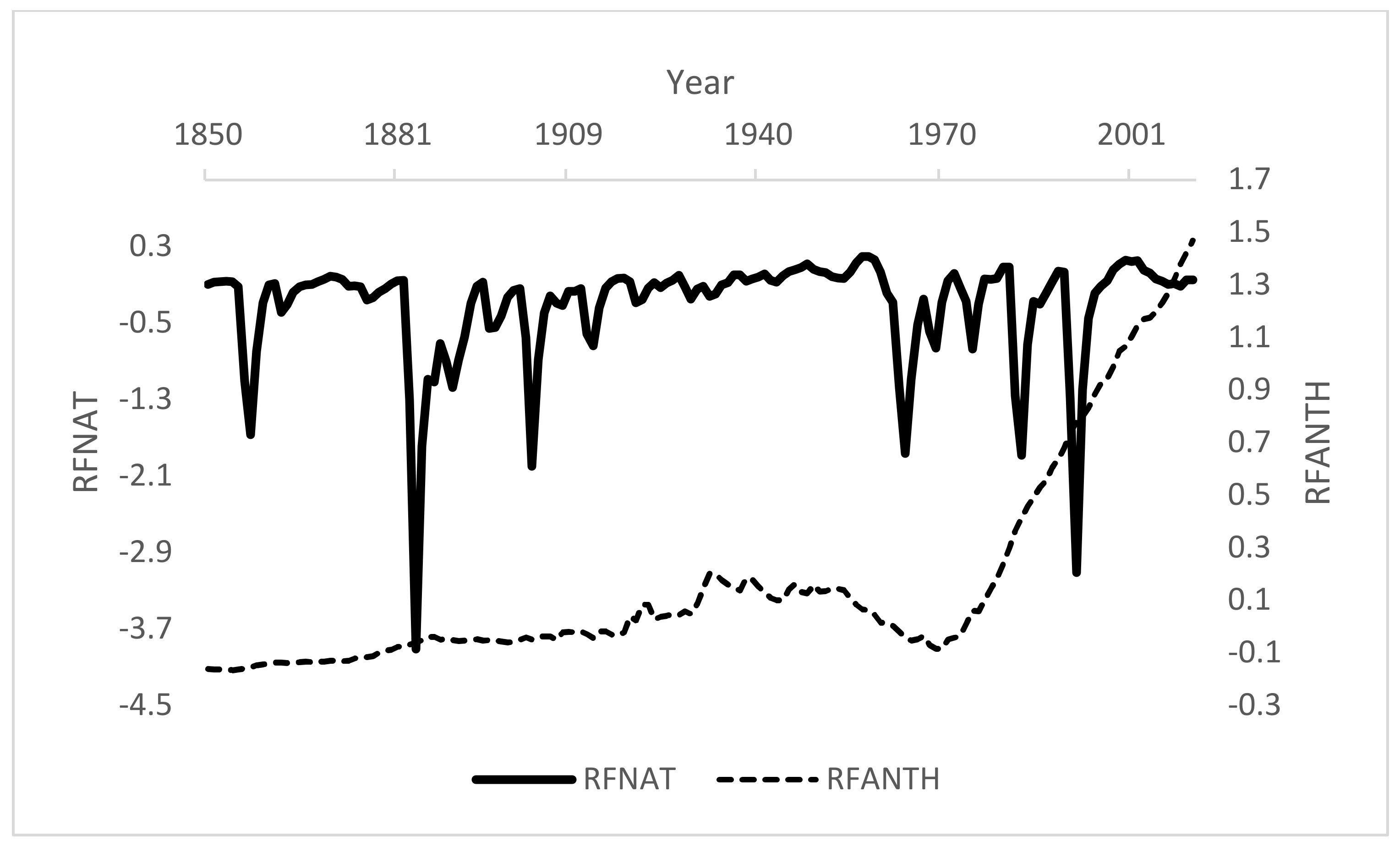
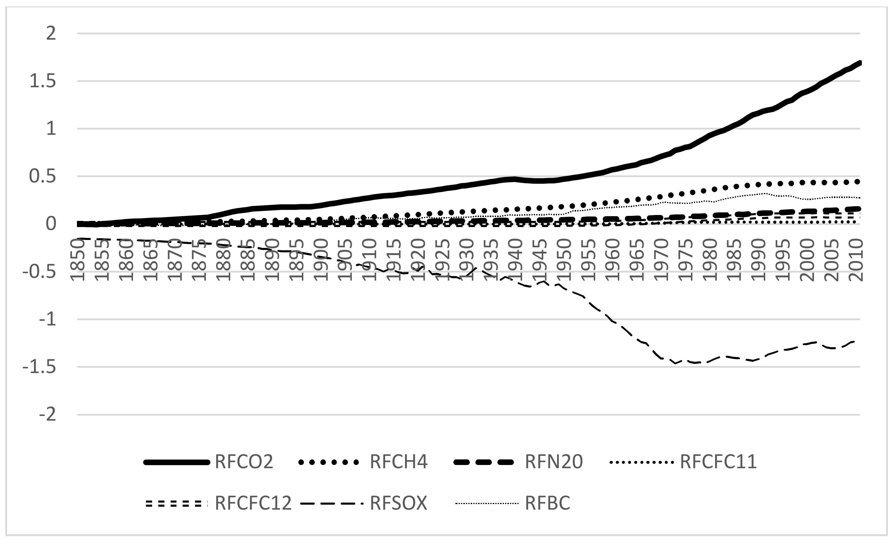
Figure 2 presents the time series of anthropogenic (solid line) and natural (dashed line) RF. The time series of anthropogenic RF had an increasing trend until 1950, decreased between 1951 and 1970, and then sharply increased, while natural RF maintained a stable trend throughout the period between 1850 and 2015. Figure 3 presents yearly records of all sources of anthropogenic RF. CFCs, methane and black and organic carbon emissions stopped increasing in the 1990s, while sulfur emissions sharply decreased between 1950 and 1975. In addition to CO emissions, dinitrogen oxide emissions also increased throughout and beyond the decade of the 1990s; however, dinitrogen oxide emissions only slightly increased and, at their highest level in 2006, were less than the size of the RF due to CO emissions.
Taken together, Figure 1 and Figure 2 show that the increase in CO emissions could have played an important role in the increase in global temperature. In order to measure the causal impact of the increase in CO emissions on global temperature, we use the increase in CO emissions in 1960 as the treatment that could have affected the temperature time series, and, accordingly, define the years between 1850 and 1959 as the pre-treatment period, and the years between 1960 and 2011 as the post-treatment period. We then estimate a BSTS model where the response series is the time series of temperature anomalies and it is a function of all natural and anthropogenic RF variables. We use the model to predict the counterfactual, that is, the time series of temperature anomalies in the post-treatment period if radiative forcing due to CO emissions had remained stable at the 1959 level. For every year between 1960 and 2011, the difference between the actual time series of temperature anomalies and the counterfactual series provides a causal estimate of the impact of CO emissions on global temperature.
3. Model
The most general BSTS model can be described with the following two equations:
where and are independently distributed. Equation (1) defines the relationship between the response time series and a latent d-dimensional state vector . Equation (2) describes how the state vector evolves over time. is a d-dimensional vector of hyperparameters, is the transition matrix containing the hyperparameters that determine the evolution of the state variables, and is a control matrix. is the error vector of the measurement equation, and is the q-dimensional error vector of the state equation with . The vector is built by concatenating the individual state components, and and are blocks of diagonal matrixes.
3.1. Prior Distributions and Elicitation
The approach used for inference is Bayesian and therefore requires to specify a prior distribution over the model parameters and a distribution over the initial state values. Let be the set of model parameters and the state vector. We specify a prior distribution over the model parameters and a distribution over the initial state values, and we sample from using Markov chain Monte Carlo (MCMC). Most of the state components depend only on a small set of variance parameters that govern the diffusion of the individual state components. A typical prior distribution for such variance parameter is:
where G is the Gamma distribution. When many potential controls are available, the model will choose an appropriate subset of controls by placing a spike-and-slab prior over coefficients, which assigns a zero value (spike) to an unknown subset of coefficients, and a weakly informative distribution on the complementary set of nonzero coefficients (slab, usually a Gaussian with a large variance).
3.2. Inference
Posterior inference can be divided into three main steps. First, we simulate draws of the model’s parameters and the state vector given the observed data in the pre-treatment period. Second, we use a Gibbs sampler to simulate a sequence of the model’s parameters and state vectors from a Markov chain whose stationary distribution is . We simulate from the posterior predictive distribution over the counterfactual time series given the observed pre-treatment observations . Third, we use the posterior predictive samples to compute the posterior distribution of the pointwise impact for each time point in the post-treatment period, that is for .
The main object of interest is the posterior incremental effect, that is, the counterfactual time series of y that would have been observed after the treatment if the treatment had not taken place, . This posterior predictive density is defined as a joint distribution over all counterfactual data points, rather than as a collection of pointwise univariate distributions, which ensures that we correctly account for the serial structure in the pre-treatment data to simulate the trajectory of counterfactuals [13].
For each draw and for each time point , we set
which produces samples from the approximate posterior predictive density of the effect attributed to the treatment.
4. Estimation
In order to use the BSTS model to compute the causal impact of CO emissions on global temperature, we use the increase in CO emissions in 1960 as the treatment that could have affected the temperature time series, and accordingly defined the years between 1850 and 1959 as the pre-treatment period, and the years between 1960 and 2011 as the post-treatment period. We set as the time series of average global temperature between 1850 and 2011, and we model it as a function of the matrix , which includes all sources of natural and anthropogenic RF, that is, two variables on natural RF due to volcanic eruptions and solar activity and the six variables of anthropogenic RF due to sulfur emissions, black and organic carbon emissions, methane, dinitrogen oxide, CFC11 and CFC12. Because of their high correlation, emissions due to methane, dinitrogen oxide, CFC11 and CFC12 were summed together in one greenhouse gases emissions variable. Finally, in addition to the sources of natural and anthropogenic RF, we also include ocean heat content since the oceans store most of the increase in heat due to RF [17]. We assume that all covariates in the matrix have time-invariant coefficients; thus we set and .
One important advantage of a BSTS model is that we do not have to commit to a fixed set of covariates that we choose a priori as equivalently important explanatory variables. Rather, the spike-and-slab prior described in Section 3.1 allows us to integrate out posterior uncertainty about how strongly each covariate should influence our predictions, which avoids overfitting. In other words, the posterior predictive distribution depends only on the observed data and the priors, and not on parameter estimates or on the inclusion or exclusion of specific covariates, all of which have been integrated out. Thus, as discussed by [13], through Bayesian model averaging, we commit neither to any particular set of covariates, which helps avoiding an arbitrary selection, nor to point estimates of their coefficients, which prevents overfitting.
In order to build the simplest possible model, we assume that all covariates have a contemporaneous effect on the outcome variable. we also assume no seasonal component in the response series, and we do not explicitly model a local linear trend since local linear trends in BSTS models used to make long-term predictions often result in implausibly wide uncertainty intervals [13].
Finally, since we are building a Bayesian model, we specify a prior distribution over the model parameters and a distribution over the initial state values, and we sampled from using MCMC. We set the prior standard deviation of the Gaussian random walk of the local level at the default value of , and we estimate the model using 1000 MCMC samples.
The BSTS methodology identifies the average effect of the treatment on the treated, and it is an example of the train, test, treat and compare (TTTC) approach, which is an ML generalization of the classic treatment–control approach using a predictive model of the counterfactual that replaces the control group [9]. The BSTS model was trained and tested on the pre-treatment period of 1850–1959, and was then used to predict the counterfactual, that is, the yearly global temperatures during the post-treatment period (1960–2011) if RF due to carbon dioxide emissions had remained stable at the 1959 level. Finally, the time series of actual temperatures was compared to the time series of counterfactual temperatures, that is, to the time series of temperatures that would have been observed if RF due to carbon dioxide emissions had remained stable at the 1959 level. The difference between the actual and counterfactual time series in the post treatment period provides a measure of the causal effect of interest. Computationally, the model’s estimation was performed using the R package CausalImpact [18].
5. Identification and Validity
The BSTS method generalizes the differences in differences (DID) estimator to a time-series setting by modeling the counterfactual of a time series observed before and after a treatment. With respect to a standard DID estimator, the BSTS method has three main advantages. First, it does not assume i.i.d. data and is able to account for the time series structure in the pre-treatment period data to simulate the trajectory of the counterfactual series, so that the posterior predictive density (the counterfactual time series of y that would have been observed after the treatment if the treatment had not taken place) is defined as a joint distribution over all counterfactual data points. Second, it identifies how the causal impact of interest evolves over time after the treatment. Third, it does not impose restrictions on the way in which the control time series are used to estimate the counterfactual, whereas DID applications on time series data require restrictions [19].
OLS estimators could also offer a solution to the limitations of DID designs since they can account for the full counterfactual trajectory. However, they disregard the time series features of the data, and ignore posterior uncertainty about the parameters. On the contrary, the BSTS methodology precludes a rigid commitment to a specific set of covariates, which avoids overfitting [13].
The validity of the BSTS method relies on two main assumptions:
Assumption 1.
Among the X covariates that are used to estimate the counterfactual, at least one control time series is not affected by the treatment. This is a crucial assumption since control time series that receive no treatment account for the effect of other relevant factors that would otherwise remain unobserved.
Assumption 2.
During the pre-treatment period, there is a strong and stable relationship between the covariates included in the X matrix used to build the BSTS model and the response time series. This assumption is necessary to make the relationship between the response time series and the control time series stable throughout the pre- and post-treatment period.
In the context of our application, natural emissions allow the first assumption to be satisfied since there is no evidence that CO emissions affect natural emissions. Quantitatively, natural RF is mainly driven by volcanic eruptions and it follows a very different trend than anthropogenic RF. In particular, while CO emissions have been steeply increasing (bold line in Figure 1), natural RF had the same trend throughout the period between 1850 and 2011 (dashed line in Figure 2). We can also formally assess the validity of assumption 1 by testing that the time series of CO RF does not Granger cause the time series of natural RF. Since it is difficult to identify the actual data generating process and the statistical properties of the temperature and forcing time series, we followed [15] and we used the [20] Granger causality test that is robust to the presence of integrated variables and non-cointegration by including one additional lag of the variables to the standard model for each possible degree of integration. As in [15], we set to two the maximal order of integration in the data. For each component of natural RF (volcanic eruptions and solar activity), we estimated a model of the current values of natural RF as a function of its own past values and those of CO RF. For both natural RF and CO, we included the number of lags that adequately model the dynamic structure so that the coefficients of further lags are not statistically significant. For each natural RF component, the results, all available upon request, confirm that we failed to reject the null that the time series of CO RF does not Granger cause the time series of the natural RF. In addition to this, we note that identification is strengthened by the presence of several covariates that satisfy Assumption 1. If we run the same robust Granger causality test for each covariate in the X matrix, unreported results, all available upon request, show that Assumption 1 was also satisfied for all time series of anthropogenic RF except for dinitrogen oxide.
In addition to natural RF, the X matrix includes the six sources of anthropogenic RF other than carbon dioxide (sulfur emissions, black and organic carbon emissions, methane, dinitrogen oxide, CFC11 and CFC12). If we run the same robust Granger causality test for each of these six covariates, unreported results, all available upon request, show that the first assumption is satisfied for all time series of antropogenic RF except for dinitrogen oxide. Therefore, the model includes a total of six variables that satisfy Assumption 1, which strengthens identification of the model’s estimates.
For the validity of the second assumption, all covariates included in the X matrix must have a stable relationship with average global temperature both in the pre-treatment and in the post-treatment periods. We can assess the validity of this assumption by testing that the relationship between each covariate and global temperature does not have a structural break in 1960. For each variable x in the X matrix, we estimated the average global temperature as a function of its lagged values, the variable x, and the interaction term between x and a dummy variable for the time variable year ⩾1960, and we tested that the coefficient of the interaction term is not statistically significant. The results, all available upon request, confirm that no interaction term was statistically significant, which supports the assumption that each covariate included in the X matrix had a stable relationship with the temperature series before and after the year 1960.
6. Main Results
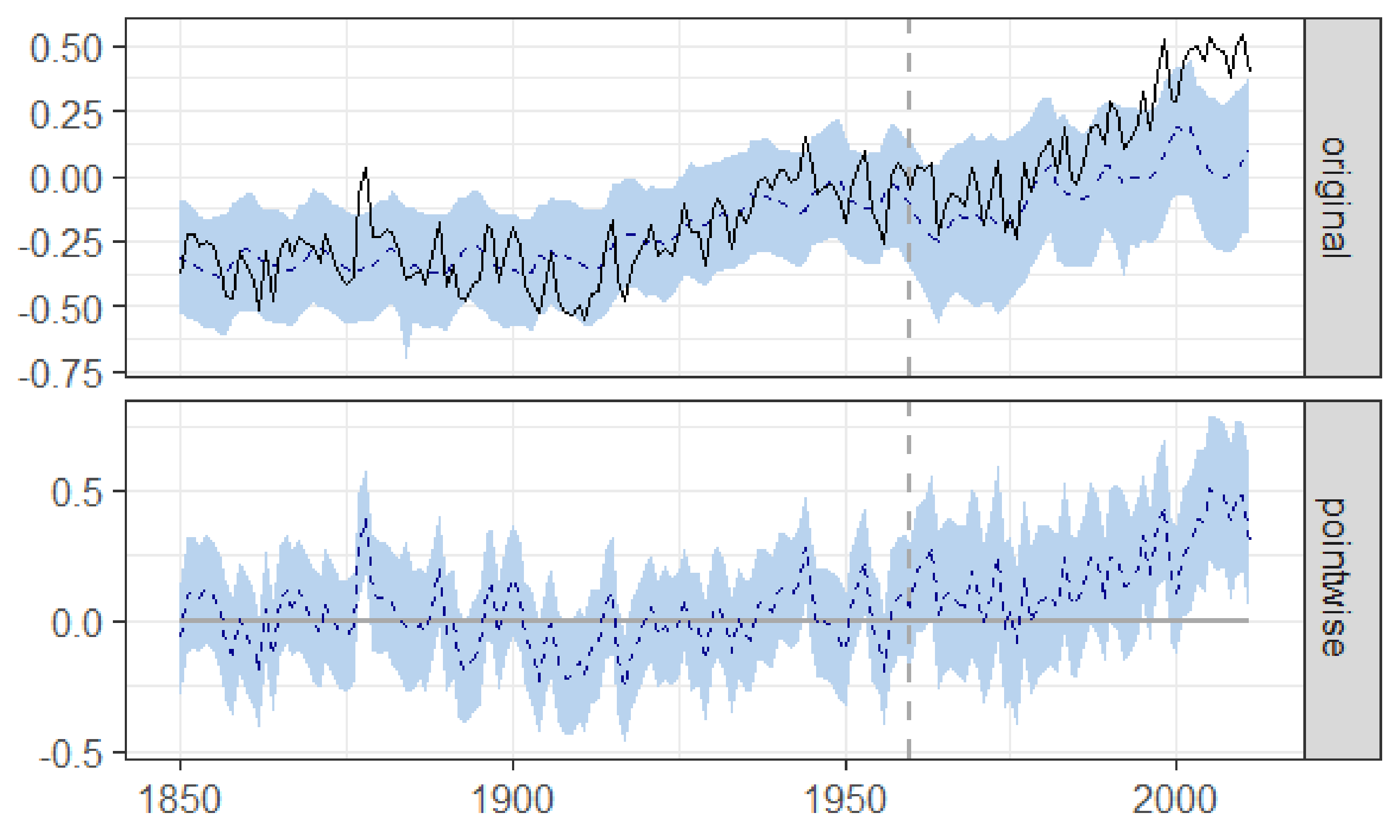
Figure 4 and Table 1 present the main results. The top panel of Figure 4 shows the actual time series of average global temperature (solid line) and the counterfactual time series of average global temperature if RF due to CO emissions had remained stable at the 1959 level (dashed line); the bottom panel of Figure 4 shows the difference between the two time series.
As expected, the impact of keeping CO emissions at the 1959 level takes some time to manifest: actual temperature anomalies first move together with the counterfactual predictions and then begin to diverge having been consistently and significantly higher since the beginning of the 1980s. The ability to identify how the effect of the treatment changes over time underscores one key advantage of the BSTS method with respect to a DID estimator that is unable to identify how the causal impact evolves with time.
Table 1 reports the actual and counterfactual average global temperature in the post-treatment period. The difference between the counterfactual and the actual average temperature () is the estimated average causal effect of CO emissions on global temperature, and it is statistically significant. In order to assess the magnitude of this effect, we estimated the counterfactual trend of the temperature between 1960 and 2011, which we compared to the trend of the actual temperature for the same period. We obtained a statistically significant estimate of for the former and a statistically significant estimate of for the latter. By taking the difference between the two trends and multiplying this average yearly effect by the number of years in the post-treatment period, we find that between 1960 and 2011 the average global temperature increased by about degrees Celsius more than it would have increased if CO emissions had remained at the 1959 level, which is a sizeable increase that is consistent with the findings from previous literature [10].
As discussed in Section 4, we estimated a BSTS model that includes all sources of anthropogenic and natural emissions that affect global temperature. One advantage of the BSTS method is that it does not require a fixed commitment to a specific set of controls by integrating out posterior uncertainty about the influence of each control variable and the uncertainty about which variables to include in the first place. Therefore, it is important to assess which predictors are informative and to which extent. We can do so by computing the inclusion probability of each control variable, that is, the posterior probability of each predictor being included in the model, which we report in Table 2 together with the estimated average coefficient, that is, the expected value of the coefficient’s posterior and its standard deviation. Table 2 shows that the most important variables are RF due to solar activity (RFSOLAR) and RF due to greenhouse gases emissions (RFGHG), which have inclusion probabilities close to 1 and are statistically significant at the 0.05 per cent level.
Robustness Checks
We perform three main robustness checks. First, we repeat the analysis using temperature data from the GISS v3 dataset, which are available in [15] since the year 1880. Second, we note that the variable ocean heat content has all null records until the year 1955, which was the effective year of data availability for this variable. we therefore first estimate the model with the outcome variable measured using GISS v3 temperature data on the 1880–2011 sample and the pre-treatment period defined as 1880–1959; second, we estimate the model on the 1955–2011 sample with the pre-treatment period defined as 1955–1959. Unreported results, all available upon request, show that, in both cases, we find consistent and very similar results.
Third, we assess the accuracy of the model’s estimates. The authors of [13] discuss the model’s accuracy in detail, and show that the impact estimates become less accurate as the forecasting post-treatment period increases since the true counterfactual becomes more and more likely to deviate from its expected trajectory. In the context of our application, we can test accuracy by assessing the sensitivity of the estimated causal impact of CO emissions when the treatment year changes, and thus the forecasting horizon changes. As discussed in the Data Section, CO emissions start increasing in 1960 and increase even more since 1975. We can therefore re-estimate the model by setting 1975 as the treatment year so that the pre-period increases by 15 years. When we do so, we find that the difference between the counterfactual and the actual average temperature is with a standard deviation of and a 95% CI . The estimated causal impact of CO emissions on global temperature is thus statistically significant and very close in magnitude to the one estimated in the baseline model (Table 1), and the results are unchanged.
7. Discussion
There are several research questions that cannot be answered using the standard social sciences’ quantitative toolkit of causal inference, since the treatment affects all subjects simultaneously. One example of this type of question is the causal impact of anthropogenic emissions on global warming. Despite a scientific consensus based on extensive evidence of the man-made nature of global warming, climate change denial is still present. The literature on climate change perceptions attributes this in part to the complexity of climate science, which incentivizes individuals to rely on the often biased information that political parties provide [12].
In this paper, we draw attention to a ML technique, which relies on a few testable assumptions to predict the missing counterfactual, and produces easily interpretable and replicable results. We find that carbon dioxide emissions are responsible for an increase of about degrees Celsius in average global temperature between 1961 and 2011, which confirms the results of an extensive literature that has assessed the impact of human emissions on global warming [10].
The main strength of the BSTS method is that it does not rely on an a priori choice of variables and functional forms, and thus does not suffer from limited robustness and generalizability. In doing this, it complements the strand of applied econometric literature that uses a theory-driven automatic model selection approach to study climate change. As a prominent example of this literature, the authors of [21] used a theory-driven automatic model selection approach to study the effect of anthropogenic activity on CO emissions. Their results show that monthly industrial production components are highly significant and consistently selected in the estimated models of CO emissions, and that fluctuations in CO are driven by anthropogenic factors. As for the BSTS method, the automatic model selection approach is not restricted to a priori selection of variables and functional forms and consistently estimates the causal impact of interest.
In this paper, we show how an ML technique can identify causal effects in settings where a randomized experiment is not feasible, and we provide one additional application of using ML to answer causal questions of policy relevance [1,2,4,5,9].
For the specific question of climate change, by applying a methodology that relies on a few directly testable assumptions, we provide robust evidence of the man-made nature of global warming, which could be used to communicate results and reduce people’s incentives to turn to biased sources of information that fuel climate change skepticism.
Funding
This research received no external funding.
Institutional Review Board Statement
Not applicable.
Informed Consent Statement
Not applicable.
Data Availability Statement
Not applicable.
Acknowledgments
I thank Valentina Angius and seminar participants at Scuola Superiore Sant’Anna, Italy, the University of Georgia, USA, the EMCC-III Conference at Villa Mondragone, and the EuroCIM Conference in Florence for several useful feedbacks and suggestions.
Conflicts of Interest
The author declares no conflict of interest.
References
- Athey, S. The Impact of Machine Learning on Economics. NBER Working Paper. 2018. Available online: http://www.nber.org/chapters/c14009.pdf (accessed on 5 May 2021).
- Sendhil, M.; Spiess, J. Machine Learning: An Applied Econometric Approach. J. Econ. Perspect. 2017, 31, 87–106. [Google Scholar]
- Einav, L.; Levin, J.D. The Data Revolution and Economic Analysis; NBER Working Paper; National Bureau of Economic Research: Cambridge, MA, USA, 2013; p. 19035. [Google Scholar]
- Einav, L.; Levin, J.D. Economics in the Age of Big Data. Science 2014, 346, 1243089. [Google Scholar]
- Varian, H.R. Big Data: New Tricks for Econometrics. J. Econ. Perspect. 2014, 28, 3–28. [Google Scholar]
- Kleinberg, J.; Ludwig, J.; Mullainathan, S.; Obermeyer, Z. Prediction Policy Problems. Am. Econ. Rev. Pap. Proc. 2015, 105, 491–495. [Google Scholar] [CrossRef] [PubMed] [Green Version]
- Chalfin, A.; Danieli, O.; Hillis, A.; Jelveh, Z.; Luca, M.; Ludwig, J.; Mullainathan, S. Productivity and Selection of Human Capital with Machine Learning. Am. Econ. Rev. Pap. Proc. 2016, 106, 124–127. [Google Scholar]
- Athey, S.; Imbens, G. The State of Applied Econometrics—Causality and Policy Evaluation. 2016. Available online: https://arxiv.org/pdf/1607.00699.pdf (accessed on 5 May 2021).
- Varian, H.R. Causal Inference in Economics and Marketing. PNAS 2016, 113, 7310–7315. [Google Scholar]
- Hegerl, G.; Zwiers, F. Use of models in detection and attribution of climate change. WIREs Clim. Chang. 2011, 2, 570–591. [Google Scholar]
- Castle, J.L.; Hendry, D.F. Climate Econometrics: An Overview. Found. Trends Econom. 2020, 10, 145–322. [Google Scholar] [CrossRef]
- Egan, P.J.; Mullin, M. Climate Change: US Public Opinion. Annu. Rev. Political Sci. 2017, 20, 209–227. [Google Scholar]
- Brodersen, K.H.; Galluser, F.; Koehler, J.; Remy, N.; Scott, S.L. Inferring Causal Impact Using Bayesian Structural Time-Series Models. Annu. Appl. Stat. 2015, 9, 247–274. [Google Scholar]
- Athey, S.; Imbens, G. Machine Leaning Methods in Economics and Econometrics. Am. Econ. Rev. Pap. Proc. 2015, 105, 476–480. [Google Scholar]
- Stern, D.I.; Kaufmann, R.K. Anthropogenic and natural causes of climate change. Clim. Chang. 2014, 122, 257–269. [Google Scholar]
- Ritchie, H.; Roser, M. CO2 and other Greenhouse Gas Emissions. 2019. Available online: https://ourworldindata.org/co2-and-other-greenhouse-gas-emissions (accessed on 5 May 2021).
- Stern, D.I. An atmosphere—Ocean multicointegration model of global climate change. Comput. Stat. Data Anal. 2006, 51, 1330–1346. [Google Scholar]
- CausalImpact 1.2.1, Brodersen et al., Annals of Applied Statistics. 2015. Available online: http://google.github.io/CausalImpact/ (accessed on 5 May 2021).
- Abadie, A.; Diamond, A.; Hainmueller, J. Synthetic control methods for comparative case studies: Estimating the effect of California’s tobacco control program. J. Am. Stat. Assoc. 2010, 105, 493–505. [Google Scholar]
- Toda, H.Y.; Yamamoto, T. Statistical inference in vector autoregressions with possibly integrated processes. J. Econom. 1995, 66, 225–250. [Google Scholar]
- Hendry, D.F.; Pretis, F. Anthropogenic influences on atmospheric CO2. In Handbook of Energy and Climate Change; Edward Elgar Publishing: Cheltenham, UK, 2013; Chapter 2; pp. 287–326. [Google Scholar]
Figure 1.
Yearly records of atmospheric concentration of CO (bold) and temperature anomalies.

Figure 2.
Yearly records of anthropogenic (bold) and natural radiative forcing.

Figure 3.
Yearly records of anthropogenic radiative forcing for carbon dioxide (RFCO2), methane (RFCH4), dinitrogen oxide (RFN20), CFC11 (RFCFC11), CFC12 (RFCFC12), sulfur emissions (RFSOX), and black and organic carbon (RFBC).
Figure 3.
Yearly records of anthropogenic radiative forcing for carbon dioxide (RFCO2), methane (RFCH4), dinitrogen oxide (RFN20), CFC11 (RFCFC11), CFC12 (RFCFC12), sulfur emissions (RFSOX), and black and organic carbon (RFBC).

Figure 4.
Yearly estimates of the causal effect of carbon dioxide RF on temperature.


Table 1.
Point estimate of the causal effect of carbon dioxide RF on temperature.
| Average | |
|---|---|
| Actual | 0.15 |
| Prediction (s.d.) | −0.045 (0.073) |
| 95% CI | [−0.18, 0.1] |
| Absolute effect (s.d.) | 0.2 (0.073) |
| 95% CI | [0.053, 0.34] |
| Posterior tail-area probability p: 0.007 | |
| Posterior probability of a causal effect: 99.3% | |
Table 2.
Inclusion probability, estimated average coefficient and standard deviation of each control variable included in the model.
Table 2.
Inclusion probability, estimated average coefficient and standard deviation of each control variable included in the model.
| Inclusion Probability | Average Coefficient (sd) | |
|---|---|---|
| Ocean Heat Content | 0.049 | 0.001 (0.022) |
| RFBC | 0.221 | −0.113 (0.273) |
| RFSOX | 0.704 | 0.579 (0.465) |
| RFGHG | 0.961 | 0.940 (0.399) |
| RFSOLAR | 0.976 | 0.425 (0.123) |
| RFVOL | 0.378 | 0.072 (0.101) |
Note: RFGHG = RFCH4 + RFN2O + RFCFC11 + RFCFC12
Publisher’s Note: MDPI stays neutral with regard to jurisdictional claims in published maps and institutional affiliations. |
© 2021 by the author. Licensee MDPI, Basel, Switzerland. This article is an open access article distributed under the terms and conditions of the Creative Commons Attribution (CC BY) license (https://creativecommons.org/licenses/by/4.0/).
Share and Cite
MDPI and ACS Style
Binelli, C. Estimating Causal Effects When the Treatment Affects All Subjects Simultaneously: An Application. Big Data Cogn. Comput. 2021, 5, 22. https://0-doi-org.brum.beds.ac.uk/10.3390/bdcc5020022
AMA Style
Binelli C. Estimating Causal Effects When the Treatment Affects All Subjects Simultaneously: An Application. Big Data and Cognitive Computing. 2021; 5(2):22. https://0-doi-org.brum.beds.ac.uk/10.3390/bdcc5020022
Chicago/Turabian StyleBinelli, Chiara. 2021. "Estimating Causal Effects When the Treatment Affects All Subjects Simultaneously: An Application" Big Data and Cognitive Computing 5, no. 2: 22. https://0-doi-org.brum.beds.ac.uk/10.3390/bdcc5020022