Adaptive Neural Network Sliding Mode Control for Nonlinear Singular Fractional Order Systems with Mismatched Uncertainties

Abstract

This paper focuses on the sliding mode control (SMC) problem for a class of uncertain singular fractional order systems (SFOSs). The uncertainties occur in both state and derivative matrices. A radial basis function (RBF) neural network strategy was utilized to estimate the nonlinear terms of SFOSs. Firstly, by expanding the dimension of the SFOS, a novel sliding surface was constructed. A necessary and sufficient condition was given to ensure the admissibility of the SFOS while the system state moves on the sliding surface. The obtained results are linear matrix inequalities (LMIs), which are more general than the existing research. Then, the adaptive control law based on the RBF neural network was organized to guarantee that the SFOS reaches the sliding surface in a finite time. Finally, a simulation example is proposed to verify the validity of the designed procedures.

1. Introduction

Fractional order systems (FOSs) have been developed greatly in the past few decades. When the fractional order $\alpha$ is equal to the integer, the FOSs reduce to integer order systems. Therefore, FOSs have more extensive applications in real life, such as image processing [1], economics [2], and robotics [3]. Stability is fundamental to FOSs. A basic theorem of asymptotic stability for FOSs is first proposed in [4] with fractional order $0<\alpha <2$. But it is difficult to use this theory to design controllers to make the FOSs stable in practical application. So, many scholars have carried out further research on FOSs. In [5], the Mittag–Leffler stability definition of FOSs is introduced and the fractional order Lyapunov method is presented. Sabatier et al. propose the linear matrix inequalities (LMIs) condition of asymptotic stability of FOSs in [6]. Necessary and sufficient conditions of robust stability and stabilization of fractional order interval systems with fractional order $\alpha$: $0<\alpha <1$ case and $1<\alpha <2$ case are developed in [7,8], respectively. Zhang et al. in [9] present a D-stability based LMI condition, which does not include complex variables. Liang et al. in [10] introduce the bounded real lemma of FOSs to solve $H_{\infty }$ control problem. In [11], Shen et al. analyze the nonlinear FOSs and put forward some significant results.

In control systems, state variables often cannot represent physical variables in a natural way to provide a mathematical model. This leads to a singular system model [12]. Therefore, singular systems are necessary to be studied. In [13], the robust stabilization of uncertain singular time-delay systems is considered, and sufficient conditions are given to ensure the system is regular, impulse-free, and asymptotically stable. In [14], by designing the controller to convert the singular system into a normal system, Ren et al. investigate the problem of guaranteed cost control for uncertain singular systems. The LMI condition for the $H_{\infty }$ control of discrete stochastic Markovian jump singular systems with state delay is constructed in [15]. As for singular fractional order systems (SFOSs), many important theoretical results have been published [16,17,18]. In [19], on the basis of [9], Three necessary and sufficient conditions are introduced to solve the admissibility problem of SFOSs. In [20], Zhang et al. investigate the problem of admissibility of T-S fuzzy SFOSs. A number of results about the output feedback controller design for SFOSs are presented in [21,22,23]. In addition, Wei et al. in [24] consider the observer design for uncertain SFOSs. When the uncertainties occur in derivative matrix E, any small disturbance may destroy the admissibility of SFOSs, which has a more serious effect than the disturbance in the system matrix. In [25], a proportional-plus derivative state feedback strategy is proposed to make such systems admissible.

Sliding mode control (SMC) is a kind of special nonlinear control in essence. It has the characteristics of fast response, insensitivity to parameter change and disturbance. Compared with backstepping technique [26,27], the SMC scheme is an effective control way to deal with nonlinearities and uncertainties of systems [28]. By design the integral sliding surface, Wang et al. in [29] study the adaptive SMC for the T-S fuzzy singular systems. The SMC technique is used to control the horizontal position of quadcopters [30,31]. The sliding mode fault tolerant control problem for nonlinear systems with actuator faults is considered in [32,33,34]. SMC is also an effective control strategy for nonlinear stochastic systems [35] and discrete systems [36]. On the basis of previous research, Edwards et al. summarize the theory and application of SMC and put forward many important theories [37]. In terms of FOSs, SMC for fractional order chaotic systems has been well investigated [38,39]. In [40], Wang et al. find that the control law based on the fractional order reaching law can reduce the time for the FOSs to reach the sliding surface. Li et al. in [41] design the sliding mode observer for SFOSs. However, the references mentioned above are conservative to a certain extent. The restricted condition of the nonlinear term of the system is required in these references. For example, in [41], the authors assume that the nonlinear terms $f_i(t,x(t))$ satisfy the norm bounded conditions $\Vert f_i(t,x(t))\Vert \le {\beta }_{1i}+{\beta }_{2i}\Vert y(t)\Vert .$ The restricted conditions are hard to achieve in practice. A radial basis function (RBF) neural network strategy can be well combined with the SMC scheme to solve this defect [42]. It is noted that the RBF neural network can approximate continuous nonlinear function with arbitrary precision [43]. The assumption that the norm of the nonlinear term is bounded can be removed. Song in [44] study the adaptive RBF neural network SMC problem for singularly perturbed systems. In [45], the admissibility of T-S fuzzy singular systems is considered by using a RBF neural network sliding mode observer. The RBF neural network SMC problems are also studied for robot manipulators [46] and the fault diagnosis of the quadcopter [47]. In summary, RBF neural network has been a very popular and mature theory. This method in used in this paper.

Motivated by above discussions, the adaptive RBF neural network SMC scheme for SFOSs with mismatched uncertainties is presented. The contributions of this paper are summarized as follows:

• A new necessary and sufficient condition for admissibility of SFOSs is presented, which contains no equality constraints.
• By expanding the dimension of the SFOS, a new sliding surface is constructed.
• Based on RBF neural network method, $\widehat{f}(t,\overline{x}(t))$ is constructed to estimate the nonlinear term $f(t,\overline{x}(t))$. The restricted assumption that $f(t,\overline{x}(t))$ is norm bounded in [41] is removed.
• The adaptive control law is exploited to guarantee that the SFOS reaches the sliding surface in a finite time.

The paper is arranged as follows: The preliminaries are provided in Section 2. In Section 3, the sliding mode control scheme is presented. In Section 4, a simulation example is given to prove the validity of the proposed method. Finally, in Section 5, the conclusion is obtained.

Throughout this paper, ${\mathbb{R}}^n$ denotes the n-dimensional real vectors. ${\mathbb{R}}^{n\times m}$ is the m by n real matrices. $M^{\mathrm{T}}$ is the transpose of matrix $M.$ Tr$(X)$ denotes the trace of matrix X. $X>0(<0)$ means that the matrix X is positive (negative) definite, $\mathrm{sym}(Y)$ denotes the expression $Y+Y^T$, * indicates the symmetric part of a matrix, $a=sin\left(\frac{a\pi }{2}\right),b=cos\left(\frac{a\pi }{2}\right)$, $\Vert ·\Vert$ denotes the Euclidean norm of vectors. The $\alpha$th order Caputo fractional derivative of $f(t)$ is defined as

$$D^{\alpha }f(t)=\frac{1}{\mathsf{\Gamma }(n-\alpha )}{\int }_0^t{(t-\tau )}^{\alpha +1-n}{f}^{(n)}(\tau )\mathrm{d}\tau ,$$

where $n-1<\alpha <n,$ $n\in {\mathbb{N}}_{+}$ and $\mathsf{\Gamma }(·)$ is the Gamma function.

2. Preliminaries

Consider the nonlinear SFOS,

$$\begin{array}{c}\hfill \begin{array}{c}(E+\mathsf{\Delta }E)D^{\alpha }x(t)=(A+\mathsf{\Delta }A)x(t)+B(u(t)+f(t,x(t)),\hfill \end{array}\end{array}$$

(1)

where $x(t)\in {\mathbb{R}}^n$ is the system state, $u(t)\in {\mathbb{R}}^l$ is the control input, and $\alpha (0<\alpha <1)$ is the fractional order, $E\in {\mathbb{R}}^{n\times n}$ is a singular matrix such that rank$(E)=r<n$. $A\in {\mathbb{R}}^{n\times n}$, $B\in {\mathbb{R}}^{n\times l}$ are constant matrices. $\mathsf{\Delta }A,\mathsf{\Delta }E\in {\mathbb{R}}^{n\times n}$ are uncertain matrices, which is assumed to be of the form

$$\left[\mathsf{\Delta }A\mathsf{\Delta }E\right]=UF(\sigma )\left[V_1{V}_2\right],$$

where U, $V_1$, $V_2$ are known constant matrices. The uncertain matrix $F(\sigma )$ satisfies $F^{\mathrm{T}}(\sigma )F(\sigma )\le I,$ where $\sigma \in \mathsf{\Phi },$$\mathsf{\Phi }$ is a compact set in $\mathbb{R}$. Besides, the unknown function $f(t,x(t))\in {\mathbb{R}}^l$ represents the nonlinear term. Let $\overline{x}(t)={\left[x^{\mathrm{T}}(t)D^{\alpha }{x}^{\mathrm{T}}(t)\right]}^{\mathrm{T}},$ SFOS (1) is rewritten as

$$\overline{E}{D}^{\alpha }\overline{x}(t)=(\overline{A}+\mathsf{\Delta }\overline{A})\overline{x}(t)+\overline{B}(u(t)+f(t,\overline{x}(t))),$$

(2)

where

$$\overline{E}=\left[\begin{array}{cc}{I}_n& 0\\ 0& 0\end{array}\right],\overline{A}=\left[\begin{array}{cc}0& I_n\\ A& -E\end{array}\right],\mathsf{\Delta }\overline{A}=\left[\begin{array}{cc}0& 0\\ \mathsf{\Delta }A& -\mathsf{\Delta }E\end{array}\right],\overline{B}=\left[\begin{array}{c}0\\ B\end{array}\right],f(t,\overline{x}(t))=f(t,x(t)).$$

In order to design the sliding mode controller for system (2), we introduce following facts and lemmas. Considering the unforced SFOS

$$E{D}^{\alpha }x(t)=Ax(t).$$

(3)

(3) is denoted as the triple $(E,A,\alpha )$.

Definition 1

([19]).

(1) 

SFOS (3) is regular if there exist a constant scalar s such that $\det (s^{\alpha }E-A)\ne 0.$

(2) 

SFOS (3) is impulse free if $\mathrm{deg}(\det (sE-A))=\mathrm{rank}(E).$

(3) 

SFOS (3) is asymptotically stable if all the finite roots of $\det (s^{\alpha }E-A)$ satisfy $\left|\arg (\mathrm{spec}(E,A,\alpha ))\right|>\alpha \frac{\pi }{2}.$

(4) 

SFOS (3) is admissible if it is regular, impulse free, and stable.

Since $\mathrm{rank}(E)=r,$ it is easy to obtain that there exist nonsingular matrices $M,N\in {\mathbb{R}}^{n\times n},$ such that

$$MEN=\left[\begin{array}{cc}{I}_r& 0\\ 0& 0\end{array}\right],MAN=\left[\begin{array}{cc}{A}_1\hfill & A_2\hfill \\ A_3\hfill & A_4\hfill \end{array}\right].$$

(4)

It is noted that (3) is equivalent to

$$\left\{\begin{array}{c}\hfill D^{\alpha }{\overline{x}}_1(t)=A_1{\overline{x}}_1(t)+A_2{\overline{x}}_2(t),\\ \hfill 0=A_3{\overline{x}}_1(t)+A_4{\overline{x}}_2(t),\end{array}\right.$$

(5)

where ${\overline{x}}_1\in {\mathbb{R}}^r,$ ${\overline{x}}_2\in {\mathbb{R}}^{n-r}$ and ${\left[{\overline{x}}_1^{\mathrm{T}}(t){\overline{x}}_2^{\mathrm{T}}(t)\right]}^{\mathrm{T}}=N^{-1}x(t).$ If $A_4$ is nonsingular, system (5) is rewritten by it equivalent representation

$$D^{\alpha }{\overline{x}}_1(t)=(A_1-A_2{A}_4^{-1}{A}_3){\overline{x}}_1(t).$$

(6)

Lemma 1

([9]). When $E=I,$ SFOS (3) is reduced to

$$D^{\alpha }x(t)=Ax(t).$$

(7)

System (7) is asymptotically stable if and only if there exist two matrices $X,Y\in {\mathbb{R}}^{n\times n},$ such that

$$\left[\begin{array}{cc}X& Y\\ -Y& X\end{array}\right]>0,$$

(8)

$$aAX+bAY+aX{A}^{\mathrm{T}}-bY{A}^{\mathrm{T}}<0.$$

(9)

Lemma 2

([19]). Let

$$\mathsf{\Sigma }=\left[\begin{array}{cc}{\mathsf{\Lambda }}_1& {\mathsf{\Lambda }}_2\\ {\mathsf{\Lambda }}_3& {\mathsf{\Lambda }}_4\end{array}\right],$$

where ${\mathsf{\Lambda }}_1,{\mathsf{\Lambda }}_2,{\mathsf{\Lambda }}_3,{\mathsf{\Lambda }}_4$ are real matrices such that $\mathsf{\Sigma }+{\mathsf{\Sigma }}^{\mathrm{T}}<0.$ Then, ${\mathsf{\Lambda }}_4$ is nonsingular and

$${\mathsf{\Lambda }}_1+{\mathsf{\Lambda }}_1^{\mathrm{T}}-{\mathsf{\Lambda }}_2{\mathsf{\Lambda }}_4^{-1}{\mathsf{\Lambda }}_3-{\mathsf{\Lambda }}_3^{\mathrm{T}}{\mathsf{\Lambda }}_4^{\mathrm{T}}{\mathsf{\Lambda }}_2^{\mathrm{T}}<0.$$

Lemma 3

([7]). There hold

$$\begin{array}{c}\hfill \mathsf{\Omega }+\mathsf{\Gamma }F\mathsf{\Theta }+{\mathsf{\Theta }}^{\mathrm{T}}{F}^{\mathrm{T}}{\mathsf{\Gamma }}^{\mathrm{T}}<0,F^{\mathrm{T}}F\le I\end{array}$$

if and only if there exists a positive scalar ϵ such that

$$\begin{array}{c}\hfill \mathsf{\Omega }+ϵ\mathsf{\Gamma }{\mathsf{\Gamma }}^{\mathrm{T}}+{ϵ}^{-1}{\mathsf{\Theta }}^{\mathrm{T}}\mathsf{\Theta }<0,ϵ>0,\end{array}$$

where $\mathsf{\Omega },\mathsf{\Gamma },\mathsf{\Theta },F$ are given matrices of appropriate dimension, and Ω is symmetric.

Lemma 4.

The SFOS (3) is admissible if and only if there exist matrices $P_1\in {\mathbb{R}}^{r\times r},P_2\in {\mathbb{R}}^{(n-r)\times m}$ and $P_3\in {\mathbb{R}}^{(n-r)\times (n-r)}$ such that

$$\left[\begin{array}{cc}\frac{P_1+P_1^{\mathrm{T}}}{2a}& \frac{P_1-P_1^{\mathrm{T}}}{2b}\\ \frac{P_1^{\mathrm{T}}-P_1}{2b}& \frac{P_1+P_1^{\mathrm{T}}}{2a}\end{array}\right]>0,$$

(10)

$$MANP+P^{\mathrm{T}}{N}^{\mathrm{T}}{A}^{\mathrm{T}}{M}^{\mathrm{T}}<0,$$

(11)

where

$$P=\left[\begin{array}{cc}{P}_1& 0\\ a{P}_2& a{P}_3\end{array}\right],$$

(12)

$M,N\in {\mathbb{R}}^{n\times n}$ are defined in (4).

Proof. 

$[\mathrm{Sufficiency}:]$ If (4) and (10)–(12) hold, it is obtained from (11) that

$$\left[\begin{array}{cc}{A}_1{P}_1+P_1^{\mathrm{T}}{A}_1^{\mathrm{T}}+a{A}_2{P}_2+a{P}_2^{\mathrm{T}}{A}_2^{\mathrm{T}}& a{A}_2{P}_3+P_1^{\mathrm{T}}{A}_3^{\mathrm{T}}+a{P}_2^{\mathrm{T}}{A}_4^{\mathrm{T}}\\ \ast & a{A}_4{P}_3+a{P}_3^{\mathrm{T}}{A}_4^{\mathrm{T}}\end{array}\right]<0.$$

(13)

The 2-2 block in (13) gives

$$a{A}_4{P}_3+a{P}_3^{\mathrm{T}}{A}_4^{\mathrm{T}}<0,$$

hence, one has $A_4$ is nonsingular. According to [19], SFOS (3) is regular and impulse-free. We define

$$\mathsf{\Sigma }=\left[\begin{array}{cc}{A}_1{P}_1+a{A}_2{P}_2& a{A}_2{P}_3\\ A_3{P}_1+a{A}_4{P}_2& a{A}_4{P}_2\end{array}\right].$$

It follows from Lemma 2 that

$$\mathrm{sym}((A_1-A_2{A}_4^{-1}{A}_3)P_1)<0.$$

(14)

We set $P_1=aX+bY,$ where X is an symmetric matrix and Y is an antisymmetric matrix. It is obtained that

$$\frac{P_1+P_1^{\mathrm{T}}}{2a}=X,\frac{P_1-P_1^{\mathrm{T}}}{2b}=Y.$$

Thus, (10) is equivalent to (8). By Lemma 1, (14) together with (10) implies system (6) is asymptotically stable. We have SFOS (3) is asymptotically stable.

[Necessity:] We assume that system (3) is admissible. According to [19], $A_4$ is nonsingular and

$$\arg \left(\mathrm{spec}\left(A_1-A_2{A}_4^{-1}{A}_3,\alpha \right)\right)>\alpha \frac{\pi }{2}.$$

(15)

By Lemma 1, there exist matrices $X,Y\in {\mathbb{R}}^{r\times r},$ such that (8) and (16) hold.

$$\mathrm{sym}((A_1-A_2{A}_4^{-1}{A}_3)(aX+bY))<0.$$

(16)

Then, by setting $P_1=aX+bY,$ we have (10) and (14) hold. Let

$$M_1=\left[\begin{array}{cc}{I}_r& -A_2{A}_4^{-1}\\ 0& I_{n-r}\end{array}\right],N_1=\left[\begin{array}{cc}{I}_r& 0\\ -A_4^{-1}{A}_3& I_{n-r}\end{array}\right],\mathsf{\Theta }=\left[\begin{array}{cc}{P}_1& 0\\ 0& -A_4^{\mathrm{T}}\end{array}\right],$$

(17)

it follows that

$$M_{1}MAN{N}_1\mathsf{\Theta }=\left[\begin{array}{cc}(A_1-A_2{A}_4^{-1}{A}_3)P_1& 0\\ 0& -A_4{A}_4^{\mathrm{T}}\end{array}\right].$$

(18)

Since $A_4$ is nonsingular, $-A_4{A}_4^{\mathrm{T}}$ is negative definite. According to (14), one has

$$\mathrm{sym}(MAN{N}_1\mathsf{\Theta }{M}_1^{-T})<0,$$

(19)

where

$$N_1\mathsf{\Theta }{M}_1^{-T}=\left[\begin{array}{cc}{P}_1& 0\\ -A_4^{-\mathrm{T}}{A}_{3}P-A_2^{-\mathrm{T}}& -A_4^{\mathrm{T}}\end{array}\right]=\left[\begin{array}{cc}{P}_1& 0\\ a\ast (-a^{-1}{A}_4^{-\mathrm{T}}{A}_{3}P-a^{-1}{A}_2^{-\mathrm{T}})& a\ast {(-a)}^{-1}{A}_4^{\mathrm{T}}\end{array}\right].$$

(20)

By selecting $-a^{-1}{A}_4^{-\mathrm{T}}{A}_{3}P-a^{-1}{A}_2^{-\mathrm{T}}=P_2,$${(-a)}^{-1}{A}_4^{\mathrm{T}}=P_3$ and $N_1\mathsf{\Theta }{M}_1^{-T}=P,$ one has (11) holds. □

Remark 1.

Stability conditions obtained in [19,41] involve the unknown antisymmetric matrix $X_2$. In effect, these conditions contain an equality constraint that $X_2^{\mathrm{T}}=-X_2$. Lemma 4 obtained in this paper does not contain equality constraint. Lemma 4 is more efficient and general than other theorems [19,24,41] because fewer variables are introduced and the complex calculation is avoided successfully.

3. Main Results

In order to presented SMC scheme for SFOS (2), the following sliding surface is constructed

$$s(t)=\overline{G}\overline{E}{D}^{\alpha -1}\overline{x}(t)-{\int }_0^t\overline{G}\overline{B}K\overline{x}(\tau )d\tau ,$$

(21)

where $\overline{G}=\left[G_1{G}_2\right],G_1,G_2\in {\mathbb{R}}^{l\times n}$ are given matrices. It is easy to see that $\overline{G}\overline{B}=G_{2}B.$ We choose the appropriate matrix $G_2$ so that $\det (G_{2}B)\ne 0.$ $K=\left[K_1{0}_{l\times n}\right]$ is a real matrix to be designed, $K_1\in {\mathbb{R}}^{l\times n}.$ When the SFOSs move on sliding surface, one has $\dot{s}(t)=0,$

$$\dot{s}(t)=\overline{G}\overline{E}{D}^{\alpha }\overline{x}(t)-\overline{G}\overline{B}K\overline{x}(t)=0,$$

(22)

this together with system (2) gives

$$\dot{s}(t)=\overline{G}(\overline{A}+\mathsf{\Delta }\overline{A})\overline{x}(t)+\overline{G}\overline{B}u(t)+\overline{G}\overline{B}f(t,\overline{x}(t))-\overline{G}\overline{B}K\overline{x}(t)=0.$$

(23)

So the equivalent control law is obtained

$$u_{eq}(t)=-{(\overline{G}\overline{B})}^{-1}\overline{G}(\overline{A}+\mathsf{\Delta }\overline{A})\overline{x}(t)-f(t,\overline{x}(t))+K\overline{x}(t).$$

(24)

By substituting (24) into system (2), we have the sliding mode dynamic (25)

$$\overline{E}{D}^{\alpha }\overline{x}(t)=(\overline{A}+\mathsf{\Delta }\overline{A})\overline{x}(t)-\overline{B}{(\overline{G}\overline{B})}^{-1}(\overline{G}\overline{A}+\overline{G}\mathsf{\Delta }\overline{A})\overline{x}(t)+\overline{B}K\overline{x}(t).$$

(25)

Letting $\tilde{G}=I_{2n}-\overline{B}{(\overline{G}\overline{B})}^{-1}\overline{G}$, one has

$$\tilde{G}=\left[\begin{array}{cc}{I}_n& 0\\ 0& I_n\end{array}\right]-\left[\begin{array}{c}0\\ B\end{array}\right]{(G_{2}B)}^{-1}\left[G_1{G}_2\right]=\left[\begin{array}{cc}{I}_n& 0\\ -B{(G_{2}B)}^{-1}{G}_1& I_n-B{(G_{2}B)}^{-1}{G}_2\end{array}\right].$$

For notational simplicity, we set ${\overline{G}}_1=-B{(G_{2}B)}^{-1}{G}_1,$ ${\overline{G}}_2=I_n-B{(G_{2}B)}^{-1}{G}_2.$ Thus, (25) is rewritten as

$$\left[\begin{array}{cc}{I}_n& 0\\ 0& 0\end{array}\right]D^{\alpha }\overline{x}(t)=\left[\begin{array}{cc}0& I_n\\ {\overline{G}}_{2}A+{\overline{G}}_2\mathsf{\Delta }A+B{K}_1& {\overline{G}}_1-{\overline{G}}_{2}E-{\overline{G}}_2\mathsf{\Delta }E\end{array}\right]\overline{x}(t).$$

(26)

Remark 2.

By choosing the appropriate matrix $G_1,$ we get that ${\overline{G}}_1-{\overline{G}}_{2}E-{\overline{G}}_2\mathsf{\Delta }E$ is nonsingular. The following theorem is presented to ensure that the sliding mode dynamic is admissible.

Theorem 1.

System (26) is admissible if and only if there exist matrices $P_1,P_2,P_3\in {\mathbb{R}}^{n\times n},$ $Z\in {\mathbb{R}}^{l\times n}$ and a scalar $ϵ>0$, such that (10) and the following LMI hold.

$$\left[\begin{array}{ccc}a{P}_2+a{P}_2^{\mathrm{T}}& a{P}_3+P_1^{\mathrm{T}}{A}^{\mathrm{T}}{\overline{G}}_2^{\mathrm{T}}+Z^{\mathrm{T}}{B}^{\mathrm{T}}+a{P}_2^{\mathrm{T}}{\overline{G}}_1^{\mathrm{T}}-a{P}_2^{\mathrm{T}}{E}^{\mathrm{T}}{\overline{G}}_2^{\mathrm{T}}& P_1^{\mathrm{T}}{V}_1^{\mathrm{T}}-a{P}_2^{\mathrm{T}}{V}_2^{\mathrm{T}}\\ \ast & a{\overline{G}}_1{P}_3+a{P}_3^{\mathrm{T}}{\overline{G}}_1^{\mathrm{T}}-a{\overline{G}}_{2}E{P}_3-a{P}_3^{\mathrm{T}}{E}^{\mathrm{T}}{\overline{G}}_2^{\mathrm{T}}+ϵ{\overline{G}}_{2}U{U}^{\mathrm{T}}{\overline{G}}_2^{\mathrm{T}}& -a{P}_3^{\mathrm{T}}{V}_2^{\mathrm{T}}\\ \ast & \ast & -ϵI\end{array}\right]<0,$$

(27)

then, we can obtain $K_1=Z{P}_1^{-1}.$

Proof. 

Under the condition of Theorem 1 and using Schur complement Lemma, (27) is equivalent to

$$\begin{array}{c}\left[\begin{array}{cc}a{P}_2+a{P}_2^{\mathrm{T}}& a{P}_3+P_1^{\mathrm{T}}{A}^{\mathrm{T}}{\overline{G}}_2^{\mathrm{T}}+Z^{\mathrm{T}}{B}^{\mathrm{T}}+a{P}_2^{\mathrm{T}}{\overline{G}}_1^{\mathrm{T}}-a{P}_2^{\mathrm{T}}{E}^{\mathrm{T}}{\overline{G}}_2^{\mathrm{T}}\\ \ast & a{\overline{G}}_1{P}_3+a{P}_3^{\mathrm{T}}{\overline{G}}_1^{\mathrm{T}}-a{\overline{G}}_{2}E{P}_3-a{P}_3^{\mathrm{T}}{E}^{\mathrm{T}}{\overline{G}}_2^{\mathrm{T}}\end{array}\right]+ϵ\left[\begin{array}{c}0\\ {\overline{G}}_{2}U\end{array}\right]\left[0U^{\mathrm{T}}{\overline{G}}_2^{\mathrm{T}}\right]\hfill \\ +{ϵ}^{-1}\left[\begin{array}{c}{P}_1^{\mathrm{T}}{V}_1^{\mathrm{T}}-a{P}_2^{\mathrm{T}}{V}_2^{\mathrm{T}}\\ a{P}_3^{\mathrm{T}}{V}_2^{\mathrm{T}}\end{array}\right]\left[V_1{P}_1-a{V}_2{P}_2-a{V}_2{P}_3\right]<0\hfill \end{array}.$$

(28)

Now, by Lemma 3, it is easy to see that

$$\mathrm{sym}\left[\begin{array}{cc}a{P}_2& a{P}_3\\ {\overline{G}}_{2}A{P}_1+BZ+a{\overline{G}}_1{P}_2-a{\overline{G}}_{2}E{P}_2+{\overline{G}}_2\mathsf{\Delta }A{P}_1-a{\overline{G}}_2\mathsf{\Delta }E{P}_2& a{\overline{G}}_1{P}_3-a{\overline{G}}_{2}E{P}_3-a{\overline{G}}_2\mathsf{\Delta }E{P}_3\end{array}\right]<0.$$

(29)

Note that $Z=K_1{P}_1$, thus, (30) is obtained

$$\mathrm{sym}(\left[\begin{array}{cc}0& I_n\\ {\overline{G}}_{2}A+{\overline{G}}_2\mathsf{\Delta }A+B{K}_1& {\overline{G}}_1-{\overline{G}}_{2}E-{\overline{G}}_2\mathsf{\Delta }E\end{array}\right]\left[\begin{array}{cc}{P}_1& 0\\ a{P}_2& a{P}_3\end{array}\right])<0.$$

(30)

Therefore, by Lemma 4, system (2) is admissible. □

Remark 3.

In [14,21], the admissibility problems are investigated for singular systems. However, the proportional-plus derivative state feedback controller is designed so that the system is normalizable. This control method is essentially a normal system solution approach instead of a singular system solution approach. In this paper, the novel SFOS solution approach is proposed.

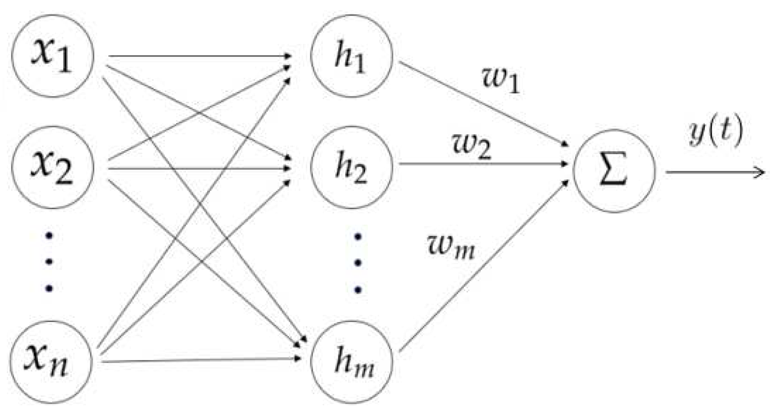
In what follows, the theorem is proposed make SFOSs satisfy the reaching condition. Besides, an RBF neural network approach is employed to deal with the nonlinear function. The RBF network structure with three hidden layers is shown in the Figure 1.

By the RBF neural network method, The nonlinear term $f(t,\overline{x}(t))$ is modeled as

$$f(t,\overline{x}(t))=W^{\mathrm{T}}h(\overline{x}(t))+{\delta }_f,$$

(31)

where $W={\left[\begin{array}{ccc}{w}_1& \cdots & w_m\end{array}\right]}^{\mathrm{T}}\in {\mathbb{R}}^{m\times l}$ is the optimal weight matrix, m is the number of neuron nodes. $h(\overline{x}(t))\in {\mathbb{R}}^m$ is the output of the Gaussian type functions, $h(\overline{x}(t))={\left[h_1(\overline{x}(t))h_2(\overline{x}(t))\cdots h_m(\overline{x}(t))\right]}^{\mathrm{T}},$ and

$$h_j(\overline{x}(t))=\exp \left(-\frac{{\Vert \overline{x}(t)-c_j\Vert }^2}{{\mu }_j^2}\right),j=1,2,\cdots ,m,$$

(32)

where $c_j={[c_{j1}{c}_{j2}\cdots c_{jn}]}^{\mathrm{T}}$ is the vector value of the center of the jth neuron and ${\mu }_j>0$ is the width of the Gaussian basis function. ${\delta }_f\in {\mathbb{R}}^l$ is the approximation error of the network, which satisfies $\Vert {\delta }_f\Vert \le \delta ,$ $\delta$ is a known constant. We use $\widehat{W}(t)$ to estimate $W^{\ast },$ and $\tilde{W}(t)=\widehat{W}(t)-W$ represents the estimation error. We set

$$\widehat{f}(t,\overline{x}(t))={\widehat{W}}^{\mathrm{T}}(t)h(\overline{x}(t))$$

(33)

to approximate $f(t,\overline{x}(t)).$ The estimation error function between $f(t,\overline{x}(t))$ and $\widehat{f}(t,\overline{x}(t))$ is defined as

$$e(t)=f(t,\overline{x}(t))-\widehat{f}(t,\overline{x}(t)).$$

(34)

Theorem 2.

System (1) moves to the sliding surface (21) in a finite time by the following adaptive SMC law:

$$u(t)={(\overline{G}\overline{B})}^{-1}(\overline{G}\overline{B}K\overline{x}(t)-\overline{G}\overline{A}\overline{x}(t)-\rho (t)\frac{s(t)}{\Vert s(t)\Vert }(-\widehat{f}(t,\overline{x}(t)),$$

(35)

where

$$\rho (t)=\lambda +\sigma \Vert \overline{G}\Vert \Vert \overline{x}(t)\Vert ,$$

(36)

λ is a positive constant, σ is the bound of the norm of the uncertain matrix $\mathsf{\Delta }\overline{A}$, which satisfies $\Vert \mathsf{\Delta }\overline{A}\Vert \le \sigma .$ The adaptive law is chosen as

$$\dot{\widehat{W}}(t)=\omega h(\overline{x}(t))s^{\mathrm{T}}(t)\overline{G}\overline{B},$$

(37)

where ω is designed as a positive constant.

Proof. 

The Lyapunov functional candidate is designed as

$$V(t)=\frac{1}{2}{s}^{\mathrm{T}}(t)s(t)+\frac{1}{2\omega }\mathrm{Tr}({\tilde{W}}^{\mathrm{T}}(t)\tilde{W}(t)).$$

(38)

Taking derivative of $V(t)$, (38) becomes

$$\dot{V}(t)=s^{\mathrm{T}}(t)((\overline{G}\tilde{A}+\tilde{G}\mathsf{\Delta }\tilde{A})\overline{x}(t)+\overline{G}\overline{B}u(t)+\overline{G}\overline{B}f(t,\overline{x}(t))-\overline{G}\overline{B}K\overline{x}(t))+\frac{1}{\omega }\mathrm{Tr}({\tilde{W}}^{\mathrm{T}}(t)\dot{\widehat{W}}(t)).$$

(39)

According to (35) and (39), (40) is obtained

$$\dot{V}(t)=s^{\mathrm{T}}(t)(\overline{G}\mathsf{\Delta }\overline{A}\overline{x}(t)-\rho (t)\frac{s(t)}{\Vert s(t)\Vert }+\overline{G}\overline{B}e(t))+\frac{1}{\omega }\mathrm{Tr}({\tilde{W}}^{\mathrm{T}}(t)\dot{\widehat{W}}(t)).$$

(40)

Thus, substituting (31), (33), (36), and (37) into (40), it follows that

$$\begin{array}{cc}\dot{V}(t)=\hfill & \Vert s(t)\Vert \Vert \overline{G}\Vert (\Vert \mathsf{\Delta }\overline{A}\Vert -\sigma )\Vert \overline{x}(t)\Vert +s^{\mathrm{T}}(t)\overline{G}\overline{B}(W^{\mathrm{T}}h(\overline{x}(t))+{\delta }_f-\widehat{W}{(t)}^{\mathrm{T}}h(\overline{x}(t)))\\ & +\mathrm{Tr}({\tilde{W}}^{\mathrm{T}}(t)h(\overline{x}(t))s^{\mathrm{T}}(t)\overline{G}\overline{B})-\lambda \Vert s(t)\Vert .\hfill \end{array}$$

(41)

Considering that

$$s^{\mathrm{T}}(t)\overline{G}\overline{B}{\tilde{W}}^{\mathrm{T}}(t)h(\overline{x}(t))=\mathrm{Tr}(s^{\mathrm{T}}(t)\overline{G}\overline{B}{\tilde{W}}^{\mathrm{T}}(t)h(\overline{x}(t)))=\mathrm{Tr}({\tilde{W}}^{\mathrm{T}}(t)h(\overline{x}(t))s^{\mathrm{T}}(t)\overline{G}\overline{B}).$$

(42)

It follows from (41) and (42) that

$$\dot{V}(t)\le -\lambda \Vert s(t)\Vert +\delta \Vert \overline{G}\overline{B}\Vert \Vert s(t)\Vert .$$

(43)

Hence, by choosing the appropriate $\lambda$ such that $\lambda -\delta \Vert \overline{G}\overline{B}\Vert =\varphi >0,$ (43) is rewritten as

$$\dot{V}(t)\le -\varphi \Vert s(t)\Vert <0,\forall \Vert s(t)\Vert \ne 0.$$

(44)

Therefore, the state trajectory of system (1) with control law (35) converges to the sliding surface (21) in a finite time. □

4. Simulation Example

This example is utilized to prove the validity of theorems 1 and 2. We consider uncertain SFOSs (1) with $\alpha =0.6$ and

$$E=\left[\begin{array}{ccc}1& 0& 0\\ 0& 1& 0\\ 0& 0& 0\end{array}\right],A=\left[\begin{array}{ccc}-3& 6& 4\\ -1& 3& 2\\ 3& 5& 4\end{array}\right],B=\left[\begin{array}{c}1\\ 1\\ 1\end{array}\right],U={\left[\begin{array}{c}1\\ 0\\ 0\end{array}\right]}^{\mathrm{T}},$$

$$V_1=\left[\begin{array}{ccc}2& 4& 6\end{array}\right],V_2=\left[\begin{array}{ccc}0.1& 0& 0\end{array}\right].$$

The system nonlinearity $f(t,x(t))$ is assumed to be $x_{1}sin(x_1(t))$ and $G_1,G_2$ are chosen as $G_1=\left[\begin{array}{ccc}1& 1& 1\end{array}\right]$ and $G_2=\left[\begin{array}{ccc}1& 1& 2\end{array}\right],$ respectively. Now, it is obtained that a set of solutions to the LMIs in (10) and (27) as follows

$$P_1=\left[\begin{array}{ccc}0.4894& 0.0746& -0.2180\\ -0.0122& 0.8121& -0.4094\\ -0.1631& -0.5117& 0.4602\end{array}\right],P_2=\left[\begin{array}{ccc}-0.8372& 1.1917& 6.7398\\ -1.2525& -0.6139& -0.8990\\ -6.7398& 0.8990& -0.7791\end{array}\right],$$

$$P_3=\left[\begin{array}{ccc}-0.8398& -2.8558& -3.3495\\ 0.2087& 0.3848& -0.6844\\ 8.5856& 1.1226& 2.9914\end{array}\right],Z=\left[\begin{array}{ccc}0.3528& 0.4067& -2.1462\end{array}\right],ϵ=1.3348.$$

Therefore, a desired matrix $K_1$ is calculated as

$$K_1=\left[\begin{array}{ccc}-3.7864& -7.3260& -12.9738\end{array}\right].$$

Thus, system (25) is admissible. By SMC law (35), system (1) moves to the sliding surface (21) in a finite time.

Furthermore, we select

$$x(0)={\left[\begin{array}{ccc}-1& -2& 0.58\end{array}\right]}^{\mathrm{T}}.$$

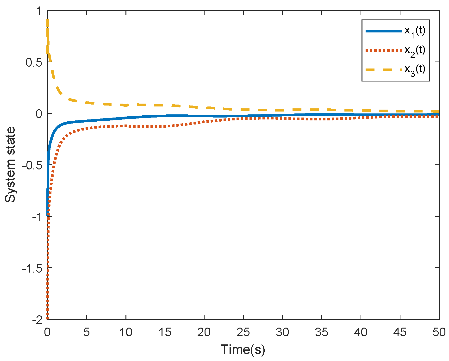
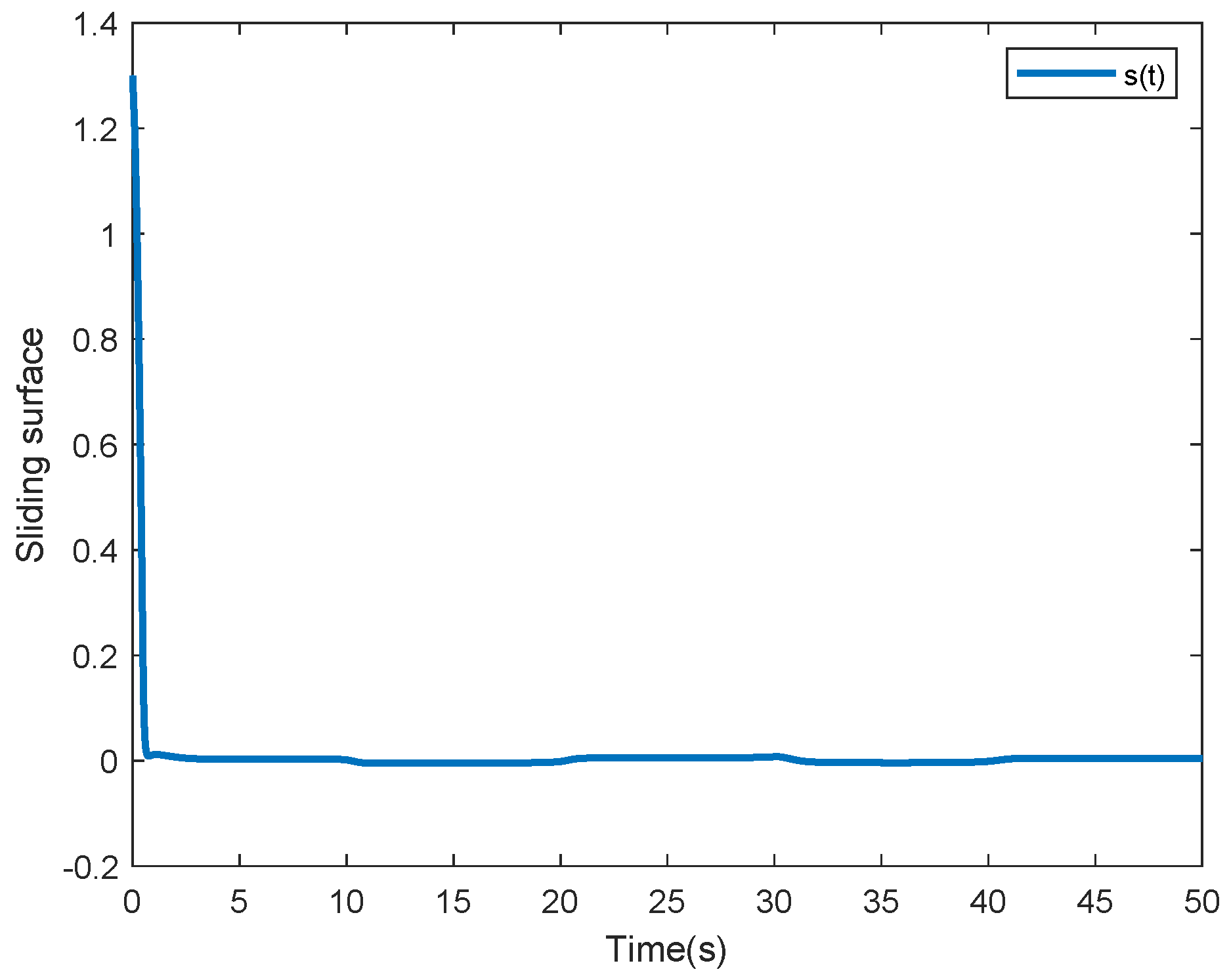
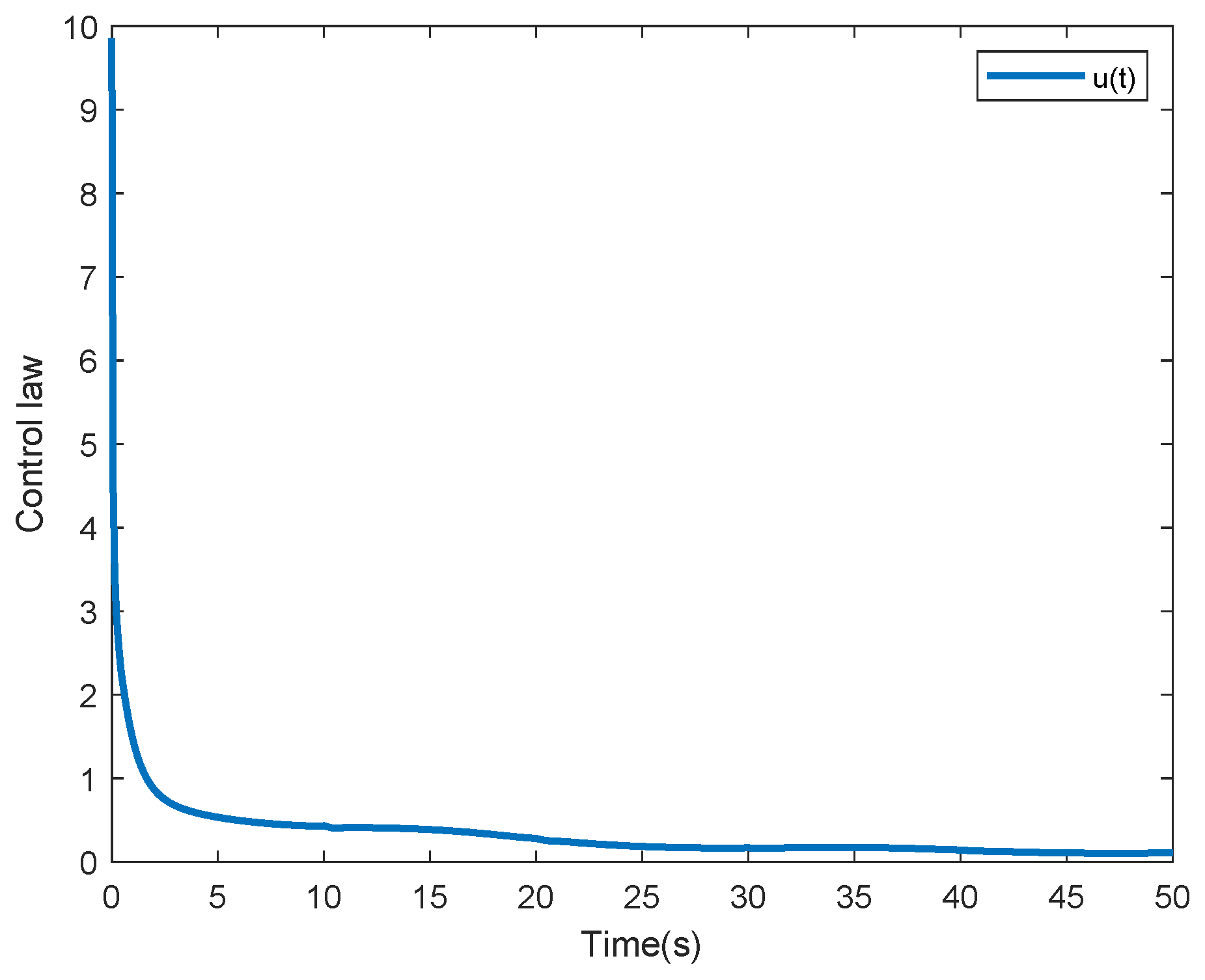
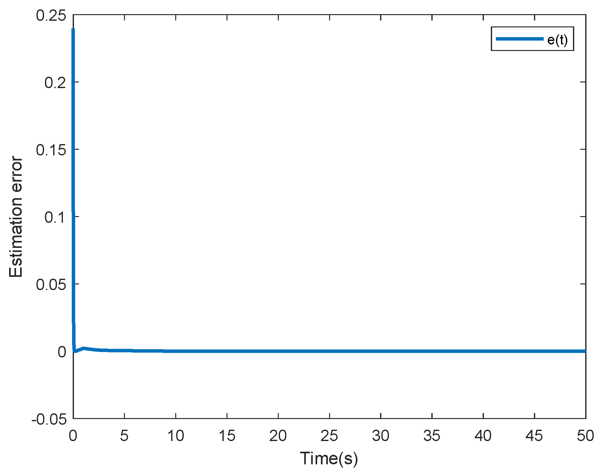
The neural network parameters are selected as $m=5,$ ${\mu }_j=0.2,$ and $c_{ji}$ is uniformly distributed in $[-2,2]$. The state response of system (1) with adaptive SMC law $u(t)$ is displayed in Figure 2. Figure 3 shows the state response of system (1) without SMC law. Compared Figure 2 with Figure 3, it is easy to see that the designed control scheme is effective. Figure 4 shows the surface function $s(t)$. Figure 5 depicts the control input $u(t).$ It is easy to see that the nonlinear term $f(t,\overline{x}(t))$ is well estimated by $\widehat{f}(t,\overline{x}(t))$ from Figure 6.

5. Conclusions

This paper investigated the issue of adaptive SMC for mismatched uncertain SFOSs. The new necessary and sufficient condition for the admissibility of SFOSs is developed, which is strict LMIs. The integral sliding mode surface with expanded dimension is constructed so that mismatched uncertainty does not exist in the derivative matrix of the sliding mode dynamic. By RBF neural network method, the adaptive control law is devised to make SFOSs satisfy the reaching condition. The restrictive assumption that the nonlinearity $f(t,x(t))$ is norm bounded is removed. In the further, the issues of SMC for SFOSs with time delay will be studied.

References

- Li, D.Z.; Tian, X.Y.; Jin, Q.B.; Hirasawa, K. Adaptive fractional-order total variation image restoration with split Bregman iteration. ISA Trans. 2018, 82, 210–222. [Google Scholar] [CrossRef]
- Su, X.; Yu, K.S.; Yu, M. Research on early warning algorithm for economic management based on Lagrangian fractional calculus. Chaos Solitons Fractals 2019, 128, 44–50. [Google Scholar] [CrossRef]
- Guo, Y.X.; Ma, B.L. Global sliding mode with fractional operators and application to control robot manipulators. Int. J. Control 2017, 92, 1497–1510. [Google Scholar] [CrossRef]
- Matignon, D. Stability properties for generalized fractional differential systems. In Proceedings of the IMACS-SMC, Lille, France, 9–12 July 1996. [Google Scholar]
- Li, Y.; Chen, Y.Q.; Podlubuy, I. Stability of fractional-order nonlinear dynamic systems: Lyapunov direct method and generalized Mittag-Leffler stability. Comput. Math. Appl. 2010, 59, 1810–1821. [Google Scholar] [CrossRef] [Green Version]
- Sabatier, J.; Moze, M.; Farges, C. LMI stability conditions for fractional order systems. Comput. Math. Appl. 2010, 59, 1594–1609. [Google Scholar] [CrossRef]
- Lu, J.G.; Chen, Y.Q. Robust stability and stabilization of fractional-order interval systems with the fractional order α: 0 < α < 1 case. IEEE Trans. Autom. Control 2010, 55, 152–158. [Google Scholar]
- Lu, J.G.; Chen, G.R. Robust stability and stabilization of fractional-order interval systems: An LMI approach. IEEE Trans. Autom. Control 2009, 54, 1294–1299. [Google Scholar]
- Zhang, X.F.; Chen, Y.Q. D-stability based LMI criteria of stability and stabilization for fractional order systems. In Proceedings of the ASME 2015 International Design Engineering Technical Conference and Computers and Information in Engineering Conference, Boston, MA, USA, 2–5 August 2015. [Google Scholar]
- Liang, S.; Wei, Y.H.; Pan, J.W.; Gao, Q.; Wang, Y. Bounded real lemmas for fractional order systems. Int. J. Autom. Comput. 2015, 12, 192–198. [Google Scholar] [CrossRef] [Green Version]
- Shen, J.; Lam, J. Non-existence of finite-time stable equilibria in fractional-order nonlinear systems. Automatica 2014, 50, 547–551. [Google Scholar] [CrossRef]
- Dai, L. Singular Control Systems; Springer: Berlin, Germany, 1989. [Google Scholar]
- Xu, S.Y.; Lam, J.; Zou, Y.; Li, J.Z. Roubst admissibility of time-varying singular systems with commensurate time delays. Automatica 2009, 45, 2714–2717. [Google Scholar] [CrossRef]
- Ren, J.C.; Zhang, Q.L. Robust normalization and guaranteed cost control for a class of uncertain descriptor systems. Automatica 2012, 48, 1693–1697. [Google Scholar] [CrossRef]
- Ma, Y.C.; Jia, X.R.; Zhang, Q.L. Robust observer-based finite-time H∞ control for discrete-time singular Markovian jumping system with time delay and actuator saturation. Nonlinear Anal. Hybrid Syst. 2018, 28, 1–22. [Google Scholar] [CrossRef]
- Ibrir, S.; Bettayeb, M. New sufficient conditions for observer-based control of frational order uncertain systems. Automatica 2015, 59, 216–223. [Google Scholar] [CrossRef]
- Marir, S.; Chadli, M.; Bouagada, D. A novel approach of admissibility for singular linear continuous-time fractional-order systems. Int. J. Control. Autom. Syst. 2017, 15, 959–964. [Google Scholar] [CrossRef]
- Lin, C.; Chen, B.; Shi, P.; Yu, J.P. Necessary and sufficient conditions of observer-based stabilization for a class of fractional-order descriptor systems. Syst. Control Lett. 2018, 112, 31–35. [Google Scholar] [CrossRef]
- Zhang, X.F.; Chen, Y.Q. Admissibility and robust stabilization of continuous linear singular fractional order systems with the fractional order α: The 0 < α < 1 case. ISA Trans. 2017, 82, 42–50. [Google Scholar]
- Zhang, X.F.; Zhao, Z.L. Normalization and stabilization for rectangular singular fractional order T-S fuzzy systems. Fuzzy Sets Syst. 2020, 381, 140–153. [Google Scholar] [CrossRef]
- Wei, Y.H.; Tse, P.W.; Yao, Z.; Wang, Y. The output feedback control synthesis for a class of singular fractional order systems. ISA Trans. 2017, 69, 1–9. [Google Scholar] [CrossRef]
- Zhan, T.; Liu, X.Z.; Ma, S.P. A new singular system approach to output feedback sliding mode control for fractional order nonlinear systems. J. Frankl. Inst. 2018, 355, 6746–6762. [Google Scholar] [CrossRef]
- Zhang, Q.H.; Lu, J.Q. Robust stability of output feedback controlled fractional-order systems with structured uncertainties in all system coefficient matrices. ISA Trans. 2020, 105, 51–62. [Google Scholar] [CrossRef] [PubMed]
- Wei, Y.H.; Wang, J.C.; Liu, T.Y.; Wang, Y. Sufficient and necessary conditions for stabilizing singular fractional order systems with partially measurable state. J. Frankl. Inst. 2019, 356, 1975–1990. [Google Scholar] [CrossRef] [Green Version]
- Ren, J.C.; Zhang, Q.L. Robust H∞ control for uncertain descriptor systems by proportional-derivative state feedback. Int. J. Control 2010, 83, 89–96. [Google Scholar] [CrossRef]
- Nguyen, A.T.; Xuan-Mung, N.; Hong, S.K. Quadcopter adaptive trajectory tracking control: A new approach via backstepping technique. Appl. Sci. 2019, 9, 3873. [Google Scholar] [CrossRef] [Green Version]
- Xuan-Mung, N.; Hong, S.K. Robust backstepping trajectory tracking control of a quadrotor with input saturation via extended state observer. Appl. Sci. 2019, 9, 5184. [Google Scholar] [CrossRef] [Green Version]
- Yan, X.G.; Edwards, C. Adaptive sliding-mode-observer-based fault reconstruction for nonlinear systems with parametric uncertainties. IEEE Trans. Ind. Electron. 2008, 55, 4029–4036. [Google Scholar]
- Wang, Y.Y.; Gao, Y.B.; Karimi, H.R.; Shen, H.; Fang, Z.J. Sliding mode control of fuzzy singularly perturbed systems with application to electric circuit. IEEE Trans. Syst. Man Cybern. Syst. 2018, 48, 1667–1675. [Google Scholar] [CrossRef]
- Xuan-Mung, N.; Hong, S.K. Improved altitude control algorithm for quadcopter unmanned aerial vehicles. Appl. Sci. 2019, 9, 2122. [Google Scholar] [CrossRef] [Green Version]
- Mung, N.; Hong, S.K. Robust adaptive formation control of quadcopters based on a leader- follower approach. Int. J. Adv. Robot. Syst. 2019, 16, 1–11. [Google Scholar]
- Zhao, Y.; Wang, J.H.; Yan, F.; Shen, Y. Adaptive sliding mode fault-tolerant control for type-2 fuzzy systems with distributed delays. Inf. Sci. 2019, 473, 227–238. [Google Scholar] [CrossRef]
- Zhang, J.X.; Yang, G.H. Prescribed performance fault-tolerant control of uncertain nonlinear systems with unknown control directions. IEEE Trans. Autom. Control 2017, 62, 6529–6535. [Google Scholar] [CrossRef]
- Zhang, J.X.; Yang, G.H. Fault-tolerant output-constrained control of unknown Euler-Lagrange systems with prescribed tracking accuracy. Automatica 2020, 111, 108606. [Google Scholar] [CrossRef]
- Gao, Q.; Feng, G.; Xi, Z.Y.; Wang, Y.; Qiu, J.B. A new design of robust H∞ sliding mode control for uncertain stochastic T–S fuzzy time-delay systems. IEEE Trans. Cybern. 2014, 9, 1556–1566. [Google Scholar] [CrossRef] [PubMed]
- Su, X.J.; Liu, X.X.; Shi, P.; Yang, R.N. Sliding mode control of discrete-time switched systems with repeated scalar nonlinearities. IEEE Trans. Autom. Control 2017, 62, 4604–4610. [Google Scholar] [CrossRef]
- Edwards, C.; Spurgeon, S.K. Sliding Mode Control: Theory and Applications; Taylor: London, UK, 1998. [Google Scholar]
- Yin, C.; Dadras, S.; Zhong, S.M.; Chen, Y.Q. Control of a novel class of fractional-order chaotic systems via adaptive sliding mode control approach. Appl. Math. Model. 2013, 37, 2469–2483. [Google Scholar] [CrossRef]
- Nian, F.Z.; Liu, X.M.; Zhang, Y.Q. Sliding mode synchronization of fractional-order complex chaotic system with parametric and external disturbances. Chaos Solitons Fractals 2018, 116, 22–28. [Google Scholar] [CrossRef]
- Wang, J.; Shao, C.F.; Chen, Y.Q. Fractional order sliding mode control via disturbance observer for a class of fractional order systems with mismatched disturbance. Mechatronics 2018, 53, 8–19. [Google Scholar] [CrossRef]
- Li, R.C.; Zhang, X.F. Adaptive sliding mode observer design for a class of T-S fuzzy descriptor fractional order systems. IEEE Trans. Fuzzy Syst. 2019, 28, 1951–1960. [Google Scholar] [CrossRef]
- Ma, X.; Sun, F.C.; Li, H.B.; He, B. Neural network-based sliding-mode control for multiple rigid-body attitude tracking with inertial information completely unknuwn. Inf. Sci. 2017, 400, 91–104. [Google Scholar] [CrossRef]
- Lin, F.J.; Shen, P.H. Robust fuzzy neural network sliding-mode control for two-axis motion control system. IEEE Trans. Ind. Electron. 2006, 4, 1209–1225. [Google Scholar] [CrossRef]
- Song, S.; Zhang, B.Y.; Song, X.N.; Zhang, Y.J.; Zhang, Z.Q.; Li, W.J. Fractional-order adaptive neuro-fuzzy sliding mode H∞ control for fuzzy singularly perturbed systems. J. Frankl. Inst. 2019, 356, 5027–5048. [Google Scholar] [CrossRef]
- Li, R.C.; Yang, Y. Sliding-mode observer-based fault reconstruction for T-S fuzzy descriptor systems. IEEE Trans. Syst. Man Cybern. Syst. 2019, 99, 2945998. [Google Scholar] [CrossRef]
- Wang, L.Y.; Chai, T.Y.; Zhai, L.F. Neural-network-based terminal sliding-mode control of robotic manipulators including actuator dynamics. IEEE Trans. Ind. Electron. 2009, 56, 3296–3304. [Google Scholar] [CrossRef]
- Xuan-Mung, N.; Hong, S.K. Barometric altitude measurement fault diagnosis for the improvement of quadcopter altitude control. In Proceedings of the 19th International Conference on Control, Automation and Systems, Jeju, Korea, 15–18 October 2019. [Google Scholar]
Figure 1.
The radial basis function (RBF) network structure.
Figure 4.
Sliding surface function .
Figure 5.
Control law .
Figure 6.
Estimation error .
Publisher’s Note: MDPI stays neutral with regard to jurisdictional claims in published maps and institutional affiliations. |
© 2020 by the authors. Licensee MDPI, Basel, Switzerland. This article is an open access article distributed under the terms and conditions of the Creative Commons Attribution (CC BY) license (http://creativecommons.org/licenses/by/4.0/).
Share and Cite
MDPI and ACS Style
Zhang, X.; Huang, W. Adaptive Neural Network Sliding Mode Control for Nonlinear Singular Fractional Order Systems with Mismatched Uncertainties. Fractal Fract. 2020, 4, 50. https://0-doi-org.brum.beds.ac.uk/10.3390/fractalfract4040050
AMA Style
Zhang X, Huang W. Adaptive Neural Network Sliding Mode Control for Nonlinear Singular Fractional Order Systems with Mismatched Uncertainties. Fractal and Fractional. 2020; 4(4):50. https://0-doi-org.brum.beds.ac.uk/10.3390/fractalfract4040050
Chicago/Turabian StyleZhang, Xuefeng, and Wenkai Huang. 2020. "Adaptive Neural Network Sliding Mode Control for Nonlinear Singular Fractional Order Systems with Mismatched Uncertainties" Fractal and Fractional 4, no. 4: 50. https://0-doi-org.brum.beds.ac.uk/10.3390/fractalfract4040050