Realization of Cole–Davidson Function-Based Impedance Models: Application on Plant Tissues

Abstract

The Cole–Davidson function is an efficient tool for describing the tissue behavior, but the conventional methods of approximation are not applicable due the form of this function. In order to overcome this problem, a novel scheme for approximating the Cole–Davidson function, based on the utilization of a curve fitting procedure offered by the MATLAB software, is introduced in this work. The derived rational transfer function is implemented using the conventional Cauer and Foster RC networks. As an application example, the impedance model of the membrane of mesophyll cells is realized, with simulation results verifying the validity of the introduced procedure.

1. Introduction

Electrical Impedance Spectroscopy (EIS) is a scientific field of great interest with a wide range of applications, particularly in characterizing biological tissues as well as different materials and interfaces [1,2,3,4,5,6,7,8,9]. A typical function that is used, in order to describe electrical impedance, is based on the Debye dielectric relaxation function and is given by (1)

$$Z_D\left(s\right)=\frac{Z_0}{1+\tau s}$$

(1)

where $Z_0$ is a characteristic impedance in $Ohms$ ($\mathrm{\Omega }$), $s=j\omega$ is the Laplacian operator, and $\tau$ is a time constant related to the material characteristic frequency ${\omega }_0$ as $\tau =1/{\omega }_0$. Despite its usefulness and popularity, this function does not take into consideration the dispersive nature of many materials, which is a result of distributed time-constants that represent the inherent built-in memory in these materials. For this reason, improved versions of the Debye function have been introduced; the first of which is the single-dispersion Cole–Cole model described by the expression in (2).

$$Z_{CC}\left(s\right)=\frac{Z_0}{1+{\left(\tau s\right)}^{\alpha }}$$

(2)

This model has been widely used in many practical applications [10,11,12,13,14,15,16,17,18]. The non-integer exponent $\alpha \in (0,1)$ is known as the dispersion coefficient and is related to the fractal structure (geometry and morphology) of the material and also to its memory behavior. Because of this exponent, the Cole–Cole model is fractional-order and its circuit implementation requires using Constant Phase Elements (CPEs; known also as fractional-order capacitors) [19,20,21,22,23,24,25]. However, there is no commercial production of fractional-order capacitors yet, and they need to be approximated using RC networks. In this regard, various methods for the approximation of the operator ${\left(\tau s\right)}^{\alpha }$ are available, such as Matsuda’s method, Continued Fraction Expansion (CFE), Oustaloup’s method, El-Khazali’s method, and others [26,27,28,29].

A second enhanced version of the Debye function is the Cole–Davidson model described by

$$Z_{CD}\left(s\right)=\frac{Z_0}{{\left(1+\tau s\right)}^{\alpha }}$$

(3)

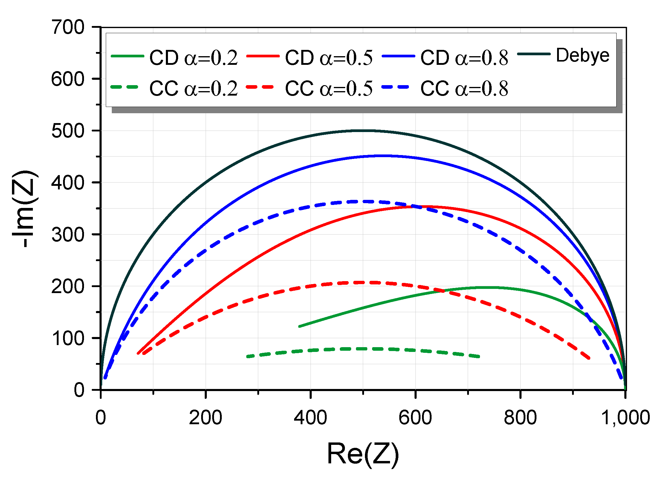
The difference between the Cole–Cole and Cole–Davidson models is illustrated through the Nyquist plots of Figure 1 [30].

It is clear that in the case of the Cole–Cole function only the operator $\left(\tau s\right)$ is raised to the power $\alpha$, while in the Cole–Davidson function the whole denominator $\left(1+\tau s\right)$ is raised to $\alpha$. For that reason, neither Constant Phase Elements nor the conventional approximation methods can be used for the realization of the Cole–Davidson impedance function.

The investigation of an alternative method, in order to approximate this type of function, is the main task and, also, the contribution of this work. MATLAB built-in functions are the key tools used in this procedure, which leads to an approximated impedance function, feasible to be implemented by simple RC networks.

The paper is organized as follows. Section 2 analytically presents the realization steps of the Cole–Davidson impedance function on circuit level. An application example in Section 3, related to the tissues of Scots Pine needles, verifies the validity of the proposed procedure through simulation results. A discussion of the conclusions and the potential applications of the presented work is given in Section 4.

2. Approximation and Implementation of the Cole–Davidson Impedance Function

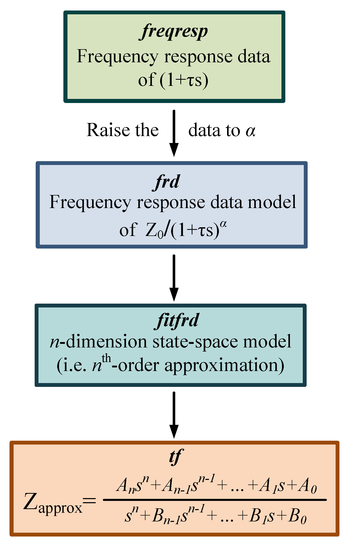
A simple method to achieve an accurate approximation of the Cole–Davidson model is to apply a curve-fitting approximation technique, exploiting appropriate built-in functions provided by the MATLAB Software. The main tools for this procedure are the commands freqresp, frd, and fitfrd, which allow the extraction and process of the frequency response data of any desired function [31,32].

Having available the parameters of the model ($Z_0,\tau ,\alpha$), obtained by using a suitable optimization algorithm applied to the experimentally measured impedance, the steps for approximating the function in (3) are as follows.

Step 1: Extract the frequency response data of the operator $\left(1+\tau s\right)$ using the freqresp built-in function.

Step 2: Raise this data to the power $\alpha$.

Step 3: Create the frequency response data model using the frd built-in function.

Step 4: Fit this frequency response data with a state-space model of n dimensions (i.e., nth-order approximation) using the fitfrd built-in function.

Step 5: Form the derived transfer function using the tf built-in function.

The block diagram in Figure 2 visualizes the above steps of the approximation process. The complexity of the procedure arises only from the fact that it is a multi-step procedure. However, its execution in MATLAB is straightforward and can be easily automated in a single script file.

At the end of this procedure, the Cole–Davidson function is transformed into a rational, integer-order transfer function of the form

$$Z_{CD,approx}\left(s\right)\cong \frac{A_n{s}^n+A_{n-1}{s}^{n-1}+\cdots +A_{1}s+A_0}{s^n+B_{n-1}{s}^{n-1}+\cdots +B_{1}s+B_0}$$

(4)

The coefficients $A_i$, $(i=0,1,...,n)$ and $B_j$, $(j=0,1,...,n-1)$ are positive real numbers, with n being the order of approximation.

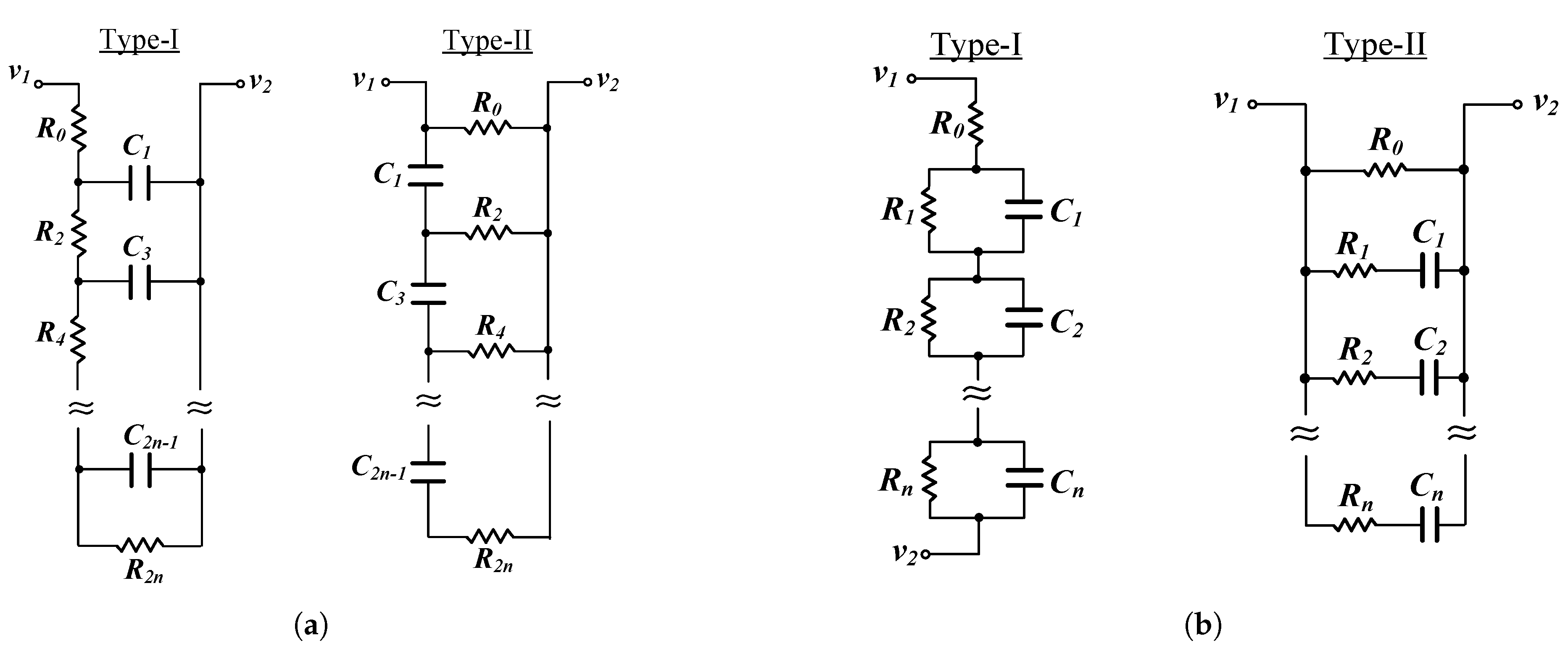
This transfer function can be easily implemented using the typical Cauer or Foster RC networks, demonstrated in Figure 3 [33]. It must be mentioned at this point that Type-I Cauer and Type-I Foster networks have similar behavior on the limits, as the impedance of both topologies at very low frequencies is equal to the series equivalent resistance of the network resistors and at very high frequencies is equal to the resistor $R_0$. A similar condition holds for Type-II Causer and Foster networks, with the corresponding impedances at very low and very high frequencies being equal to the resistor $R_0$ and the parallel connection of the network resistors, respectively.

In the case of Type-I Cauer network (Figure 3a), the expression in (4) is arranged in the form of descending powers of the variable s (starting from the highest power to the lowest power). Thus, the CFE of (4) results in

$$\begin{array}{c}\hfill Z_{CD,approx}\left(s\right)=q_0+\frac{1}{q_{1}s+\frac{1}{q_2+\frac{1}{q_{3}s+\frac{1}{.................}}}}\\ \hfill \frac{1}{q_{2n-1}s+\frac{1}{q_{2n}}}\end{array}$$

(5)

The impedance of the Type-I Cauer network in Figure 3a is given by the formula

$$\begin{array}{c}\hfill Z_{C-I}\left(s\right)=R_0+\frac{1}{C_{1}s+\frac{1}{R_2+\frac{1}{C_{3}s+\frac{1}{.................}}}}\\ \hfill \frac{1}{C_{2n-1}s+\frac{1}{R_{2n}}}\end{array}$$

(6)

and, consequently, the values of passive elements (derived by comparing the coefficients of (5) and (6)) are summarized in

Table 1. Design equations of the Cauer and Foster types of RC networks [33].

Design Equations
Cauer		Foster
Type-I	Type-II	Type-I	Type-II
$R_0=q_0$	$R_0=1/q_0$	$R_0=k$	$R_0=1/k$
$R_i=q_i,(i=2,4,...,2n)$	$R_i=1/q_i,(i=2,4,...,2n)$	$R_i=\frac{r_i}{\left|p_i\right|},(i=1,2,...,n)$	$R_i=\frac{1}{r_i},(i=1,2,...,n)$
$C_j=q_j,(j=1,3,...,2n-1)$	$C_i=1/q_j,(j=1,3,...,2n-1)$	$C_i=\frac{1}{r_i},(i=1,2,...,n)$	$C_i=\frac{r_i}{\left|p_i\right|},(i=1,2,...,n)$

.

For the Type-II Cauer network in Figure 3a, the expression in (4) is formed by arranging both the numerator and denominator in descending powers of s and performing CFE from the lowest to the highest power into the expression $Z_{CD,approx}\left(s\right)$/s. Therefore, (4) can be written as

$$\begin{array}{c}\hfill \frac{Z_{CD,approx}\left(s\right)}{s}=\frac{1}{q_{0}s+\frac{1}{q_1+\frac{1}{q_{2}s+\frac{1}{.................}}}}\\ \hfill \frac{1}{q_{2n-1}+q_{2n}s}\end{array}$$

(7)

$$\begin{array}{c}\hfill Z_{CD,approx}\left(s\right)=\frac{1}{q_0+\frac{1}{\frac{q_1}{s}+\frac{1}{q_2+\frac{1}{.................}}}}\\ \hfill \frac{1}{\frac{q_{2n-1}}{s}+q_{2n}}\end{array}$$

(8)

Comparing the coefficients of (8) and (9), the formulae for calculating the values of passive elements are as provided in Table 1.

$$\begin{array}{c}\hfill Z_{C-II}\left(s\right)=\frac{1}{\frac{1}{R_0}+\frac{1}{\frac{1}{C_{1}s}+\frac{1}{\frac{1}{R_2}+\frac{1}{.................}}}}\\ \hfill \frac{1}{\frac{1}{C_{2n-1}s}+R_{2n}}\end{array}$$

(9)

For the Type-I Foster network in Figure 3b, the Partial Fraction Expansion tool is used and (4) can be expressed as

$$Z_{CD,approx}\left(s\right)=k+\sum _{i=1}^n\frac{r_i}{s-p_i}$$

(10)

with $r_i$ and $p_i$ being the residues and poles. Meanwhile, the impedance of a Type-I Foster network is given by

$$Z_{F-I}\left(s\right)=R_0+\sum _{i=1}^n\frac{\frac{1}{C_i}}{s+\frac{1}{R_i{C}_i}}$$

(11)

Comparing the coefficients of (10) and (11), the resulting design equations are provided in Table 1.

Finally, in the case of the Type-II Foster network (Figure 3b), the expression $Y_{CD,approx}\left(s\right)/s$, where $Y_{CD,approx}\left(s\right)$ is the admittance derived from (4), is expressed using a Partial Fraction Expansion and the derived expression is

$$\frac{Y_{CD,approx}\left(s\right)}{s}=\frac{k}{s}+\sum _{i=1}^n\frac{r_i}{s-p_i}$$

(12)

or, equivalently,

$$Y_{CD,approx}\left(s\right)=k+\sum _{i=1}^n\frac{r_i·s}{s-p_i}$$

(13)

As the admittance of this network is known to be

$$Y_{F-II}\left(s\right)=\frac{1}{R_0}+\sum _{i=1}^n\frac{\frac{1}{R_i}s}{s+\frac{1}{R_i{C}_i}}$$

(14)

the equalization of the coefficients in (13) and (14) leads to the formulae in Table 1.

3. Application Example: Cell Membrane of Mesophyll Tissue in Scots Pine Needles

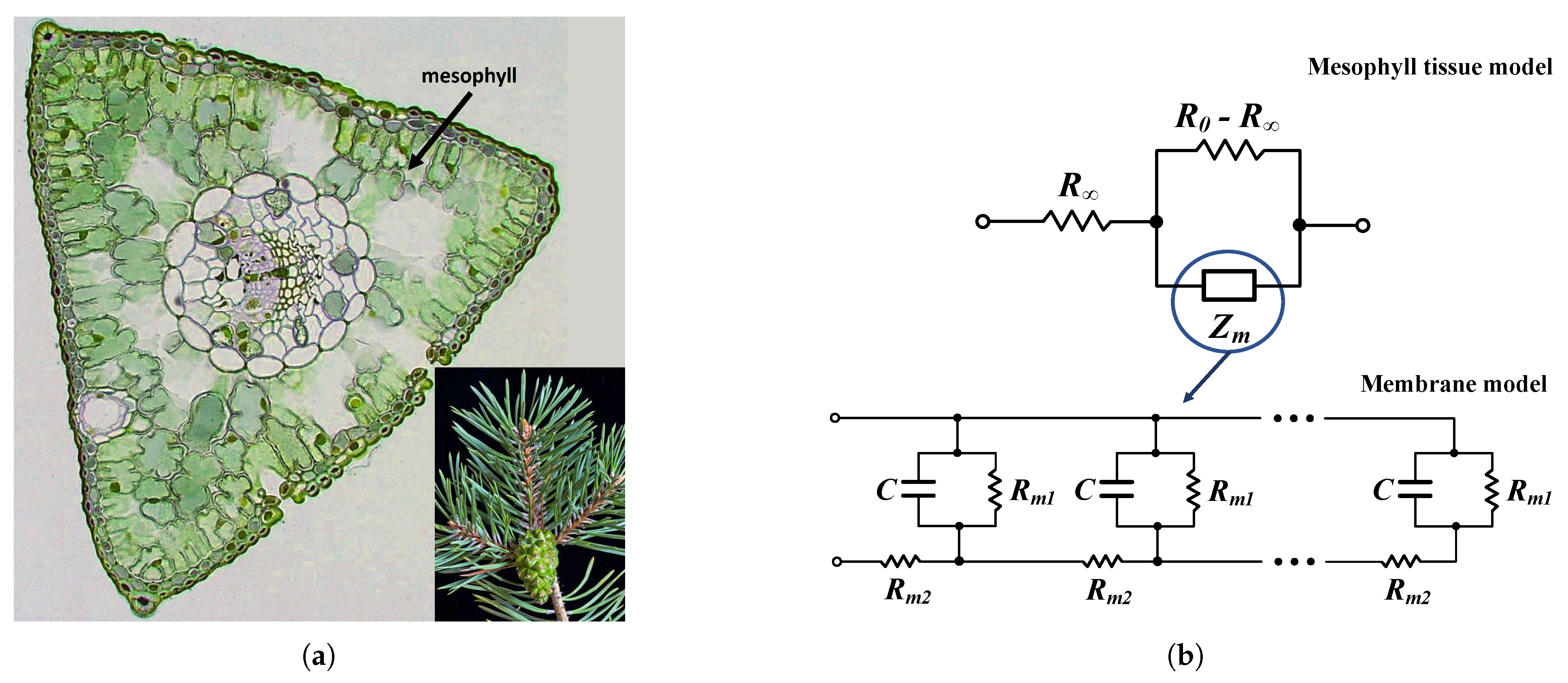
Biological tissues are composed of complexes of identical cells. The study of their function can be performed using electrical equivalents, which emulate their behavior. Considering the mesophyll tissue in Scots Pine needles, pointed out in the needle cross section in Figure 4, the electrical equivalent circuit is demonstrated in the same Figure [34]. The membrane of the tissue cells, denoted as $Z_m$ in the model, behaves as an infinite transmission line with $R_{m1}$ and C expressing a specific resistance ($\mathrm{\Omega }·$cm${}^2$) and capacitance (F/cm${}^2$), respectively, and $R_{m2}$ describing the lateral resistance in $Ohms$ ($\mathrm{\Omega }$) along a surface area of 1 cm${}^2$.

The impedance of the mesophyll tissue model is given by the expression

$$Z_t\left(s\right)=R_{\infty }+\frac{R_0-R_{\infty }}{\frac{R_0-R_{\infty }}{Z_m}+1}$$

(15)

where the coefficients $R_{\infty }$ and $R_0$ describe the extracellular and intracellular resistances of the tissue cells and $Z_m$ describes the impedance of the cells membrane.

For a mesophyll tissue of X cell layers, with each layer including Y cells, this impedance has the form of the Cole–Davidson function and is given by

$$Z_m\left(s\right)=\frac{\left(\frac{X}{Y}\right)Z_0}{{\left(1+{\tau }_{m}s\right)}^{0.5}}$$

(16)

The characteristic impedance $Z_0$ is dependent on the resistances $R_{m1}$ and $R_{m2}$ of the membrane model, while the time constant is equal to ${\tau }_m=R_{m1}C$.

Inspecting three cases of different conditions of the needles, i.e., non-infiltrated, non-hardy, and hardy stages, the parameters of the equivalent model within the frequency range $f\in \left[100,1M\right]$Hz are tabulated in

Table 2. Parameters of the Scots Pine needle equivalent model of Figure 4 [34].

Parameters	Non-Infiltrated	Non-Hardy	Hardy
$X/Y$	1/15	1/16	1/16
$R_{\infty }$ (k$\mathrm{\Omega }$)	200	95	113
$R_0$ (M$\mathrm{\Omega }$)	2.04	1.55	1.98
$Z_0$ (M$\mathrm{\Omega }$)	203	70.54	134
${\tau }_m$ (msec)	1.73	1.3	1.19

. It must be mentioned at this point that in [34] the measured spectral impedance data have been fitted to the Cole–Davidson model using a suitable optimization algorithm in order for the model parameters ($Z_0,{\tau }_m,\alpha$) to be identified. Having available these experimentally identified parameters, the aim of this work is the implementation of the electrical circuit model in Figure 4.

Applying the curve-fitting approximation method described in Section 2 on the membrane impedance function in (16), the obtained impedance functions for the three stages have the form of (4). Considering a 6th-order approximation and, indicatively, selecting the Type-I Cauer network of Figure 3a for the implementation of the functions, the values of resistors and capacitors of the network for each case are summarized in

Table 3. Values of resistors and capacitors of the Type-I Cauer network for implementing the membrane impedance model of the cases in Table 2.

Parameters	Non-Infiltrated	Non-Hardy	Hardy
$R_0$ (k$\mathrm{\Omega }$)	36.5	13.3	26.1
$R_2$ (k$\mathrm{\Omega }$)	205	75	154
$R_4$ (k$\mathrm{\Omega }$)	536	196	383
$R_6$ (k$\mathrm{\Omega }$)	1100	402	825
$R_8$ (k$\mathrm{\Omega }$)	2150	787	1540
$R_{10}$ (M$\mathrm{\Omega }$)	4.42	1.47	2.74
$R_{12}$ (M$\mathrm{\Omega }$)	4.87	1.40	2.61
$C_1$$\left(pF\right)$	1.05	2.74	1.4
$C_3$$\left(pF\right)$	3.32	8.66	4.22
$C_5$$\left(pF\right)$	7.5	19.6	10
$C_7$$\left(pF\right)$	15.4	40.2	20.5
$C_9$$\left(pF\right)$	36.5	95.3	46.4
$C_{11}$$\left(pF\right)$	147	402	196

. These values were rounded to the standard electronic component values, conforming to the E48 series defined in IEC 60063. The employed Matlab code is provided in the Appendix A, where all the cases of the Figure 3 are considered.

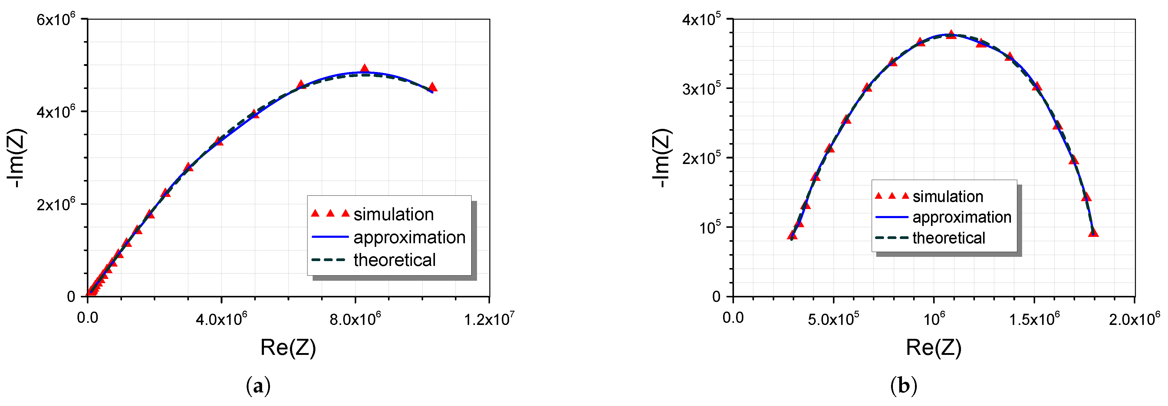
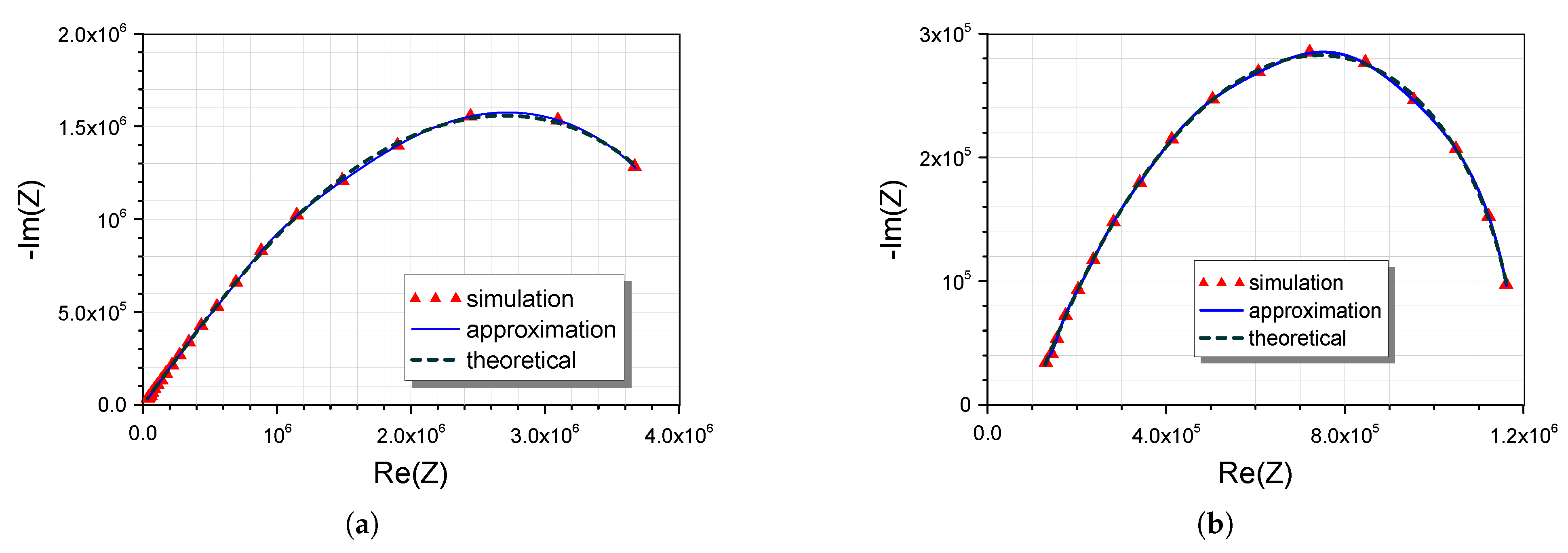
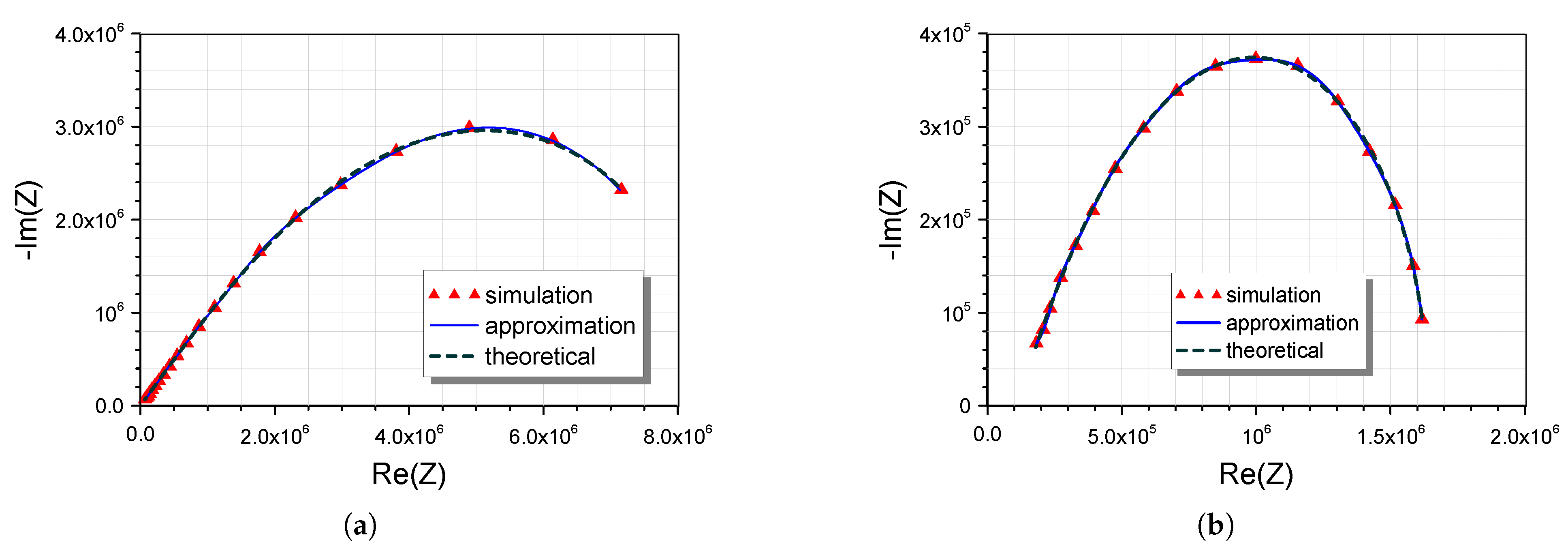
Utilizing the OrCAD PSpice simulator, the derived Nyquist plots for the membrane model, as well as the total tissue model, are presented in Figure 5 for the non-infiltrated stage, in Figure 6 for the non-hardy stage, and in Figure 7 for the hardy stage of the needle. The simulation (red triangle symbols) and approximation (blue, solid line) plots, derived using PSpice and Equation (4), respectively, converge to the theoretical (black, dashed line) plot which corresponds to the model parameters experimentally obtained in [34] in all cases. Therefore, the efficient performance of the proposed circuit implementation of the electrical membrane model as part of the whole tissue model, is confirmed.

The study of the sensitivity behavior of the network is performed using the Monte Carlo analysis tool, provided by the OrCAD PSpice simulator, for 500 runs and assuming a tolerance equal to 2%. For demonstration purposes, the case of the impedance model of the non-infiltrated stage of the needle is presented. The derived results for the impedance magnitude and phase at the center frequency $f_0$ = 10 kHz indicate mean values equal to 1.04 M$\mathrm{\Omega }$ and $-44.8°$, respectively, with the corresponding standard deviation values being 0.18 M$\mathrm{\Omega }$ and $0.62°$.

4. Discussion and Conclusions

Electrical circuit approximations of biological tissue models based on using Constant Phase Elements (CPEs) are already known in the literature. The Cole–Cole model, as well as many other models, can be constructed from combinations of passive resistors, capacitors, and CPEs [35,36]. Each CPE can be approximated using Cauer or Foster networks based on the fact that the fractional-order Laplacian operator $s^{\alpha }$ can be expressed as a rational integer-order transfer function in various ways. This, however, is not the case in the Cole–Davidson model, where an isolated operator $s^{\alpha }$ does not exist. As a result, a circuit-realizable rational integer-order impedance function cannot be derived. Having available the model parameters, extracted from spectral impedance data which are fitted to the Cole–Davidson model using any suitable optimization algorithm, we proposed in this work a novel procedure for implementing the electrical equivalent of the tissue, based on using the powerful curve fitting and state-space construction functions available in MATLAB. It must be mentioned at this point that the introduced multi-step procedure is general and can be applied to any other model. Moreover, curve fitting can be either applied to the magnitude response only, phase response only or both. The provided example of the approximation and implementation of the Cole–Davidson function of the membrane tissue of Scots Pine needles proves the validity of the proposed procedure. It must be stressed at this point that we have not introduced a novel tissue impedance model but a novel implementation procedure of the Cole–Davidson model, and we are not aware of any other circuit synthesis method available in the literature for the Cole–Davidson model. Future research is ongoing to study the feasibility of applying the proposed method on higher-order Cole–Davidson models formed of cascading multiple functions with different sets of values for ($Z_0,\tau ,\alpha$).

References

- Kun, S.; Ristic, B.; Peura, R.; Dunn, R. Real-time extraction of tissue impedance model parameters for electrical impedance spectrometer. Med. Biol. Eng. Comput. 1999, 37, 428–432. [Google Scholar] [CrossRef]
- Farinholt, K.M.; Leo, D.J. Modeling the electrical impedance response of ionic polymer transducers. J. Appl. Phys. 2008, 104, 014512. [Google Scholar] [CrossRef] [Green Version]
- Dean, D.; Ramanathan, T.; Machado, D.; Sundararajan, R. Electrical impedance spectroscopy study of biological tissues. J. Electrost. 2008, 66, 165–177. [Google Scholar] [CrossRef] [PubMed] [Green Version]
- Ionescu, C.; Desager, K.; De Keyser, R. Fractional order model parameters for the respiratory input impedance in healthy and in asthmatic children. Comput. Methods Programs Biomed. 2011, 101, 315–323. [Google Scholar] [CrossRef] [PubMed]
- Jesus, I.S.; Tenreiro Machado, J. Application of integer and fractional models in electrochemical systems. Math. Probl. Eng. 2012, 2012, 248175. [Google Scholar] [CrossRef]
- Lopes, A.M.; Machado, J.T. Modeling vegetable fractals by means of fractional-order equations. J. Vib. Control 2016, 22, 2100–2108. [Google Scholar] [CrossRef]
- Gómez-Aguilar, J.; Escalante-Martínez, J.; Calderón-Ramón, C.; Morales-Mendoza, L.; Benavidez-Cruz, M.; Gonzalez-Lee, M. Equivalent circuits applied in electrochemical impedance spectroscopy and fractional derivatives with and without singular kernel. Adv. Math. Phys. 2016, 2016, 9720181. [Google Scholar] [CrossRef] [Green Version]
- Lopes, A.M.; Machado, J.T.; Ramalho, E. On the fractional-order modeling of wine. Eur. Food Res. Technol. 2017, 243, 921–929. [Google Scholar] [CrossRef]
- Tenreiro Machado, J.; Lopes, A.M.; de Camposinhos, R. Fractional-order modelling of epoxy resin. Philos. Trans. R. Soc. A 2020, 378, 20190292. [Google Scholar] [CrossRef]
- Laufer, S.; Ivorra, A.; Reuter, V.E.; Rubinsky, B.; Solomon, S.B. Electrical impedance characterization of normal and cancerous human hepatic tissue. Physiol. Meas. 2010, 31, 995. [Google Scholar] [CrossRef]
- Vosika, Z.B.; Lazovic, G.M.; Misevic, G.N.; Simic-Krstic, J.B. Fractional calculus model of electrical impedance applied to human skin. PLoS ONE 2013, 8, e59483. [Google Scholar] [CrossRef] [PubMed] [Green Version]
- Lazarevi, M.; Caji, M. Biomechanical modelling and simulation of soft tissues using fractional memristive elements. In Proceedings of the 8th International Congress on Computational Mechanics (GRACM), Volos, Greece, 13–15 July 2015; Volume 3, pp. 1–7. [Google Scholar]
- Freeborn, T.J.; Fu, B. Fatigue-induced cole electrical impedance model changes of biceps tissue bioimpedance. Fractal Fract. 2018, 2, 27. [Google Scholar] [CrossRef] [Green Version]
- Kapoulea, S.; AbdelAty, A.M.; Elwakil, A.S.; Psychalinos, C.; Radwan, A.G. Cole-Cole Bio-Impedance Parameters Extraction From a Single Time-Domain Measurement. In Proceedings of the 2019 8th International Conference on Modern Circuits and Systems Technologies (MOCAST), Thessaloniki, Greece, 13–15 May 2019; pp. 1–4. [Google Scholar]
- Cabrera-López, J.J.; Velasco-Medina, J. Structured Approach and Impedance Spectroscopy Microsystem for Fractional-Order Electrical Characterization of Vegetable Tissues. IEEE Trans. Instrum. Meas. 2019, 69, 469–478. [Google Scholar] [CrossRef]
- Kaskouta, E.; Kapoulea, S.; Psychalinos, C.; Elwakil, A.S. Implementation of a Fractional-Order Electronically Reconfigurable Lung Impedance Emulator of the Human Respiratory Tree. J. Low Power Electron. Appl. 2020, 10, 18. [Google Scholar] [CrossRef]
- Tsikritsi, E.; Kapoulea, S.; Psychalinos, C. Implementation of the Fractional-Order Model of the Biceps Tissue During Fatigue Exercise. In Proceedings of the 2020 43rd International Conference on Telecommunications and Signal Processing (TSP), Milan, Italy, 7–9 July 2020; pp. 496–499. [Google Scholar]
- Herencsar, N.; Freeborn, T.J.; Kartci, A.; Cicekoglu, O. A Comparative Study of Two Fractional-Order Equivalent Electrical Circuits for Modeling the Electrical Impedance of Dental Tissues. Entropy 2020, 22, 1117. [Google Scholar] [CrossRef]
- Elwakil, A.S. Fractional-order circuits and systems: An emerging interdisciplinary research area. IEEE Circuits Syst. Mag. 2010, 10, 40–50. [Google Scholar] [CrossRef]
- Agambayev, A.; Farhat, M.; Patole, S.P.; Hassan, A.H.; Bagci, H.; Salama, K.N. An ultra-broadband single-component fractional-order capacitor using MoS2-ferroelectric polymer composite. Appl. Phys. Lett. 2018, 113, 093505. [Google Scholar] [CrossRef] [Green Version]
- Biswas, K.; Bohannan, G.; Caponetto, R.; Lopes, A.M.; Machado, J.A.T. Fractional-Order Devices; Springer: New York, NY, USA, 2017. [Google Scholar]
- John, D.A.; Banerjee, S.; Bohannan, G.W.; Biswas, K. Solid-state fractional capacitor using MWCNT-epoxy nanocomposite. Appl. Phys. Lett. 2017, 110, 163504. [Google Scholar] [CrossRef]
- Koton, J.; Kubanek, D.; Herencsar, N.; Dvorak, J.; Psychalinos, C. Designing constant phase elements of complement order. Analog Integr. Circuits Signal Process. 2018, 97, 107–114. [Google Scholar] [CrossRef]
- Domansky, O.; Sotner, R.; Langhammer, L.; Jerabek, J.; Psychalinos, C.; Tsirimokou, G. Practical design of RC approximants of constant phase elements and their implementation in fractional-order PID regulators using CMOS voltage differencing current conveyors. Circuits Syst. Signal Process. 2019, 38, 1520–1546. [Google Scholar] [CrossRef]
- Rezazadehshabilouyoliya, V.; Atasoyu, M.; Ozoguz, S. Emulation of a constant phase element by utilizing a lattice structure based fractional-order differentiator. AEU Int. J. Electron. Commun. 2020, 127, 153418. [Google Scholar] [CrossRef]
- AbdelAty, A.M.; Elwakil, A.S.; Radwan, A.G.; Psychalinos, C.; Maundy, B. Approximation of the Fractional-Order Laplacian sα As a Weighted Sum of First-Order High-Pass Filters. IEEE Trans. Circuits Syst. II Express Briefs 2018, 65, 1114–1118. [Google Scholar] [CrossRef]
- El-Khazali, R. On the biquadratic approximation of fractional-order Laplacian operators. Analog Integr. Circuits Signal Process. 2015, 82, 503–517. [Google Scholar] [CrossRef]
- Oustaloup, A.; Levron, F.; Mathieu, B.; Nanot, F.M. Frequency-band complex noninteger differentiator: Characterization and synthesis. IEEE Trans. Circuits Syst. I Fundam. Theory Appl. 2000, 47, 25–39. [Google Scholar] [CrossRef]
- Matsuda, K.; Fujii, H. H∞ optimized wave-absorbing control-Analytical and experimental results. J. Guid. Control. Dyn. 1993, 16, 1146–1153. [Google Scholar] [CrossRef]
- Barbé, K. Measurement of Cole–Davidson Diffusion Through Padé Approximations for (Bio) Impedance Spectroscopy. IEEE Trans. Instrum. Meas. 2019, 69, 301–310. [Google Scholar] [CrossRef]
- Bingi, K.; Ibrahim, R.; Karsiti, M.N.; Hassan, S.M.; Harindran, V.R. Fractional-Order Systems and PID Controllers: Using Scilab and Curve Fitting Based Approximation Techniques; Springer Nature: Cham, Switzerland, 2019; Volume 264. [Google Scholar]
- Ozdemir, A.A.; Gumussoy, S. Transfer function estimation in system identification toolbox via vector fitting. IFAC Pap. Online 2017, 50, 6232–6237. [Google Scholar] [CrossRef]
- Tsirimokou, G. A systematic procedure for deriving RC networks of fractional-order elements emulators using MATLAB. AEU Int. J. Electron. Commun. 2017, 78, 7–14. [Google Scholar] [CrossRef]
- Zhang, M.; Repo, T.; Willison, J.; Sutinen, S. Electrical impedance analysis in plant tissues: On the biological meaning of Cole-Cole α in Scots pine needles. Eur. Biophys. J. 1995, 24, 99–106. [Google Scholar] [CrossRef]
- Freeborn, T.J. A survey of fractional-order circuit models for biology and biomedicine. IEEE J. Emerg. Sel. Top. Circuits Syst. 2013, 3, 416–424. [Google Scholar] [CrossRef]
- Grossi, M.; Ricco, B. Electrical impedance spectroscopy (EIS) for biological analysis and food characterization: A review. J. Sens. Sens. Syst. 2017, 6, 303–325. [Google Scholar] [CrossRef] [Green Version]
Figure 1.
Nyquist plots of the Cole–Cole (CC) and Cole–Davidson (CD) impedance functions for over the frequency range f = [100,1M] Hz with = 628.3 s and = 1 k.
Figure 2.
Schematic representation of the approximation process applied to the Cole–Davidson model.
Figure 3.
Configurations of (a) Cauer and (b) Foster RC networks.
Figure 4.
Scots Pine needles (a) cross section and (b) electrical equivalent circuit of the mesophyll cell.
Figure 5.
Nyquist plots of (a) the membrane and (b) the total tissue model of the non-infiltrated stage of the Scots Pine needles.
Figure 6.
Nyquist plots of (a) the membrane and (b) the total tissue model of the non-hardy stage of the Scots Pine needles.
Figure 7.
Nyquist plots of (a) the membrane and (b) the total tissue model of the hardy stage of the Scots Pine needles.