Optimal Modelling of (1 + α) Order Butterworth Filter under the CFE Framework


Department of Electronics and Communication Engineering, National Institute of Technology Durgapur, M.G. Avenue, Durgapur 713209, India
*
Author to whom correspondence should be addressed.
Fractal Fract. 2020, 4(4), 55; https://0-doi-org.brum.beds.ac.uk/10.3390/fractalfract4040055
Submission received: 25 October 2020
/
Revised: 30 November 2020
/
Accepted: 2 December 2020
/
Published: 3 December 2020
(This article belongs to the Special Issue Fractional-Order Circuits and Systems)
Abstract
:This paper presents the optimal rational approximation of (1+α) order Butterworth filter, where α ∊ (0,1) under the continued fraction expansion framework, by employing a new cost function. Two simple techniques based on the constrained optimization and the optimal pole-zero placements are proposed to model the magnitude-frequency response of the fractional-order lowpass Butterworth filter (FOLBF). The third-order FOLBF approximants achieve good agreement to the ideal characteristic for six decades of design bandwidth. Circuit realization using the current feedback operational amplifier is presented, and the modelling efficacy is validated in the OrCAD PSPICE platform.
1. Introduction
The applications of the theory of fractional calculus (FC) in various fields of science and engineering have received significant attention from researchers in the last two decades [1]. FC generalizes the definitions of the traditional integral and derivative operators, which provides more flexibility in modelling the real-world systems [2]. Various definitions of the fractional-order derivative/integral operators are available in the literature [3]. The Riemann-Liouville definition for the fractional-order derivative of a function , where , is given as a representative in (1) [3].
where a and t are the limits of the operation; n is an integer; and denotes the gamma function.
For zero initial conditions, the Laplace transform of (1) is given by . The term is also known as the fractional-order Laplacian operator, which may represent a fractional-order differentiator (FOD) or a fractional-order integrator (FOI), for and , respectively. The frequency-domain response of is given by (2).
where is the angular frequency in radians per second (rad/s).
From (2), it can be inferred that the FOD/FOI exhibits a phase characteristic independent of the operating frequency. Several approximations of in terms of an integer-order transfer function (ITF) based on the series expansion (e.g., continued fractions expansion (CFE)), frequency-domain fitting, optimization techniques, etc., have been reported [4,5,6,7,8,9,10,11,12,13,14,15]. The accuracy of some of these approximation techniques, such as those reported in [4,5,8,12], have been compared for the design of fractional-order KHN filter in [16]. The realization of FOI/FOD using passive and active filter design techniques are also reported in [17,18]. Considering (2) from the perspective of an impedance has led to the development of the fractional-order elements (FOEs), such as the fractional-order capacitor and the fractional-order inductor . The impedance profile of a FOE can be emulated using the passive RC networks [19,20], or by active devices [21]. Fabrication of the FOEs using chemical, nanotechnology, or microelectronics technology is a dynamic area of research. An excellent recent survey paper covers the historical development and the state of the art in this regard [22].
Fractional-orders filters, being the generalization of the classical filters, can attain a precise transition band roll-off characteristic [23]. The design of fractional-order filters for the Chebyshev, inverse-Chebyshev, and elliptic types were reported in [24,25,26,27]. Fractional-order transfer function (FTF) models, which approximate the magnitude-frequency characteristic of the fractional-order lowpass [28] and bandpass [29,30] filters, were also proposed. The effectiveness of the Laguerre approximation technique for the design of fractional-order lowpass filters was demonstrated in [31]. The design and implementation of parallel fractional-order resonator systems were reported in [32]. In contrast, ITF approximants were optimally designed to model the characteristics of and order generalized lowpass, highpass, and bandpass filters in [33,34].
Butterworth filter belongs to an important class of analog filters which exhibit the maximal flatness in the magnitude response near the origin in the s-plane. The magnitude-frequency characteristic of a fractional-order lowpass Butterworth filter (FOLBF) of order is given by (3).
where is the cut-off frequency in rad/s; and .
FTF approximations of the FOLBF based on the numerical method [35], s-plane to W-plane transformation [36], least-squares curve-fitting [37], and Particle Swarm Optimization (PSO) algorithm [38] have been reported. Several FTF models of the highpass and bandpass fractional-order Butterworth filter (FOBF) were reported in [39]. Symbiotic Organisms Search algorithm based optimal FTF models for the FOBF exhibiting the highpass characteristics were proposed in [40]. In [9,38,41,42], the operator is substituted by its rational approximant in the FTF model to realize the integer-order FOLBF. In [43], the optimal ITF approximation of the order FOLBF using the Gravitational Search algorithm was demonstrated. In [44], a two-step design technique was suggested for the optimal rational approximation of the FOLBF using the Genetic Algorithm and Powell’s Conjugate Direction Algorithm (PCDA). In [45], the Colliding Bodies Optimization algorithm was used to obtain stable, rational FOLBF approximants. Comparative studies based on nine state-of-the-art nature-inspired algorithms were carried out in [46] to realize the optimal ITF models for and order FOLBFs. Optimal designs of symmetric and asymmetric type bandpass FOBFs were reported in [47,48], respectively. Optimal digital FOLBF models were recently reported in [49,50]. One of the significant challenges in an ITF-based approximation of the fractional-order filters is to achieve larger bandwidth with lower hardware overhead (design order). The approximation bandwidth for the third-order optimal models reported in [43,44] are restricted in the frequency range from 0.01–10 rad/s and 0.01–100 rad/s, respectively. Additionally, the bandwidth of the FOLBF based on the substitution method is limited by the order of the rational approximant corresponding to the operator [9].
This paper proposes two different techniques to improve the bandwidth of the third-order approximants corresponding to the order Butterworth filter. In the first approach, the CFE-based biquadratic approximation of the operator is substituted in an FTF model of the FOLBF. The coefficients of this non-optimal model are then treated as an initial point for the design variables in the optimization routine, which also employs a new cost function. The proposed method incorporates inequality constraints to ensure a stable design; thus, it requires a constrained optimization (CO) problem solver. Hence, this approach can be regarded as an optimal extension of the technique reported in [9,38,41].
In contrast, the second proposed method comprises of two design steps. At first, a scaled and shifted FOI is cascaded with a transfer function having a pole at s = −1. The center frequency of the FOI in the resultant transfer function is determined in an optimal sense by minimizing the magnitude-frequency error concerning the ideal FOLBF. Then, pole-zero optimization (PZO) is carried out to obtain the stable and minimum-phase response FOLBF using only the design variable bounds. This approach can be implemented using an unconstrained optimizer.
Comparisons with the state of the art demonstrate significant improvement in modelling accuracy of the proposed models for the design bandwidth of rad/s. Circuit implementation using the current feedback operational amplifier (CFOA) [51,52,53] is presented. SPICE simulations for the 1.5th-order FOLBF model are shown as a representative case to demonstrate the practical viability.
2. Proposed Techniques
The biquadratic approximation of the operator with a center frequency of is given by (4).
where (i = 0, 1, 2) denotes the coefficients of . The values of , , and based on the CFE technique, as reported in [9], are , , and , respectively.
2.1. First Method: Constrained Optimization
An FTF model of the FOLBF, reported in (1) of [37], is given by (5).
where the coefficients and of are expressed as a function of as per (6) and (7), respectively.
Substituting (4) in (5) leads to an integer-order model of the form (8).
where ; ; ; ; ; ; ; and = 1 rad/s.
The proposed rational approximant of the order FOLBF is defined by (9).
where is a scalar number which denotes the coefficient terms of the numerator and denominator polynomials of .
The FOLBF design can be formulated as an optimization (minimization) problem, with the fitness function proposed in (10).
subject to
where rad/s; rad/s; L (=1000) denotes the number of sampled frequency points which are logarithmically spaced in the interval rad/s; and represents the decision variable vector. The initial points provided to the optimizer are given by The inequality constraints, as shown in (11) and (12), are formulated using the Routh-Hurwitz criteria [54] to ensure stable and minimum-phase response of the proposed approximant.
2.2. Second Method: Pole-Zero Optimization
Consider the transfer function as defined by (13).
where is used to ensure dB.
The optimal value of , i.e., , is evaluated by conducting the single variable optimization (minimization) of two different objective functions, as proposed by (14) and (15).
The proposed FOLBF approximant is modelled by (16).
where k is the gain; (i = 1, 2) and (i = 1, 2, 3) denote the zeros and poles, respectively, of .
The optimal model is then determined by minimizing the fitness function, as proposed in (17).
subject to , , and .
It may be noted that these constraints can be satisfied by setting the boundary values of the decision variables only. The vector of decision variables is represented as . The initial points for the design variables are given by (18)–(21).
3. Simulation Results and Discussions
The optimization algorithms to minimize (10) and (17) are implemented in MATLAB (software: MATLAB 2014a) using the following framework-Solver: fmincon (algorithm: ‘active-set’); maximum number of objective function evaluations allowed (MaxFunEvals) = 50,000; termination tolerance on the fitness function value (TolFun) = 1 × 10⁻¹⁰; termination tolerance on the decision variable (TolX) = 1 × 10⁻¹⁰; and maximum number of iterations allowed (MaxIter) = 50,000. In the case of (14) and (15), the MATLAB function fminbnd (with search bounds in the range [0, 1000]) is used to determine the optimal value of . The lower bound (Lb) and upper bound (Ub) of the decision variable k for the PZO are set as 0 and 100, respectively; for the other design variables, the Lb and Ub are chosen as 0 and , respectively. The Lb and Ub of the decision variables for the CO technique are set as 0 and 1000, respectively.
3.1. Modelling Performance
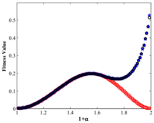
The FOLBF models, for varying from 0.01 to 0.99 in steps of 0.01, are designed using both the proposed approaches. The error fitness values (f1 and f4) yielded for the designs are compared in Figure 1. It is found that: (i) the solution quality for the PZO method is the same irrespective of the two different evaluation techniques for ; (ii) the same accuracy is attained by the FOLBFs designed using the PZO and the CO methods for ; and (iii) for , the CO method achieves a better modelling accuracy than PZO.
The initial points for the 1.2nd-, 1.5th-, and 1.8th-order FOLBFs based on the CO method are obtained as [1.6000 4.9600 2.4000 2.4000 7.0979 7.3986 2.5384], [1.0000 4.7500 3.0000 3.0000 7.5458 8.2765 3.3318], and [0.4000 4.3600 3.6000 3.6000 8.7459 9.4521 3.9187], respectively. The corresponding optimal models are given by (22)–(24), respectively.
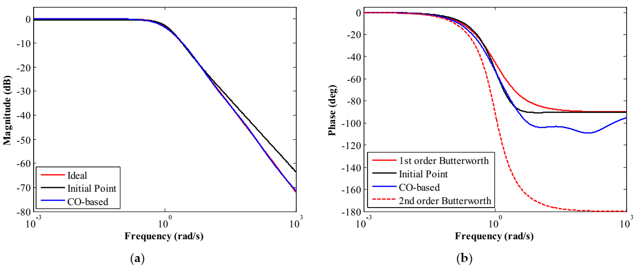
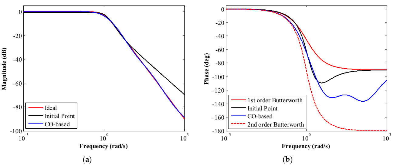
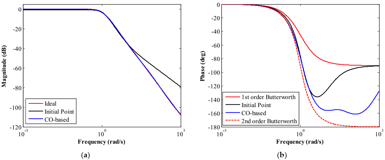
The magnitude and phase plots of the CO-based 1.2nd-, 1.5th-, and 1.8th-order FOLBFs are shown in Figure 2, Figure 3 and Figure 4, respectively. The responses of the models before optimization (i.e., the initial point) are also presented in the corresponding figures. It can be observed that the optimal designs demonstrate close agreement to the ideal magnitude-frequency characteristic for six decades of frequency. Since the FOLBFs are defined in terms of the magnitude function, their ideal phase characteristic is undefined. However, it is well-known that as , the first- and second-order Butterworth filters attain the phase value of and , respectively. Hence, it is expected that the phase of the order Butterworth filter will be , as . From the phase plots, it can be seen that as , the initial point yields a phase value of which is similar to that of the first-order Butterworth filter. For the proposed models, although fractional-stepping in the phase characteristic is exhibited, however, the responses display significantly large ripples in the higher frequencies and deviate considerably from the desired theoretical value when . Specifically, the phase values for the proposed 1.2nd-, 1.5th-, and 1.8th-order models at rad/s are obtained as , , , respectively. It may be noted that the cost function (10) does not consider the phase characteristic; hence, the proposed approximants can attain good magnitude response accuracy only. The coefficients of the CO-based 1.01–1.99th-order FOLBFs are presented in the Appendix A (Table A1).
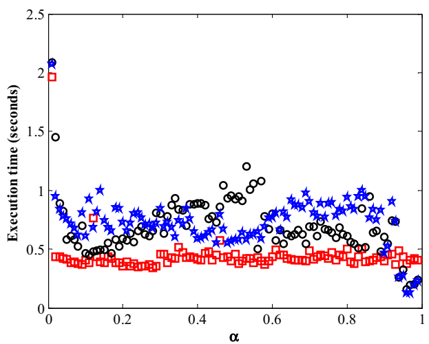
The execution times for the CO- and PZO-based optimization routines are compared in Figure 5. Both the PZO methods consume a higher execution time than CO for all the design orders, except 0.12 and 0.94–0.99. It may be recalled that similar to the CO, PZO also solves for seven design variables, where one decision variable is obtained using either (14) or (15), and six others are yielded from (17). Overall, the CO method may be regarded as a computationally faster and more accurate method to solve the proposed FOLBF approximation problem.
3.2. Determination of Generalized Expressions for Model Coefficients
This section investigates the modelling performance where the coefficients of the CO-based FOLBFs are represented as a function of For this purpose, the rational approximant as given by (9) is expressed by (25).
The polynomial expression in terms of for the coefficient (j = 1, 2, …, 6) is approximated using (26).
where the coefficients are generated using the MATLAB function polyfit. The values of the coefficients for the polynomial expression corresponding to m = 12 for to are presented in Table 1. The norm of residuals (normr), which is a measure of the accuracy of approximation between the actual and the curve-fitted data points, is also presented in Table 1. A lower value of normr indicates a smaller error between the original (optimal) value of the coefficient and the polynomial approximation.
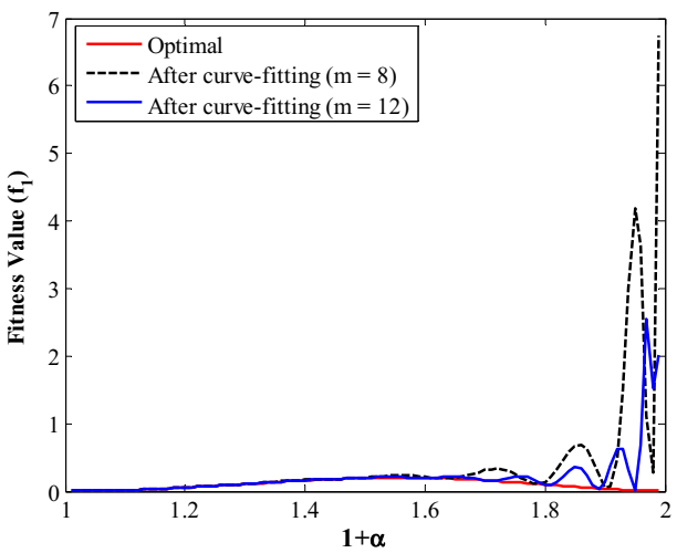
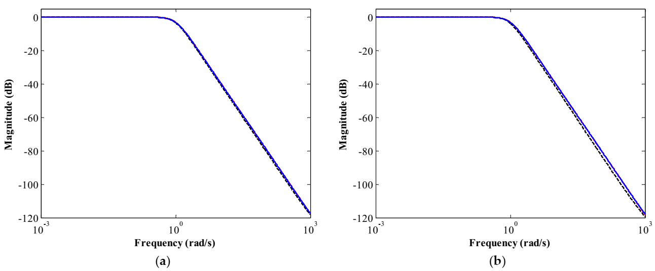
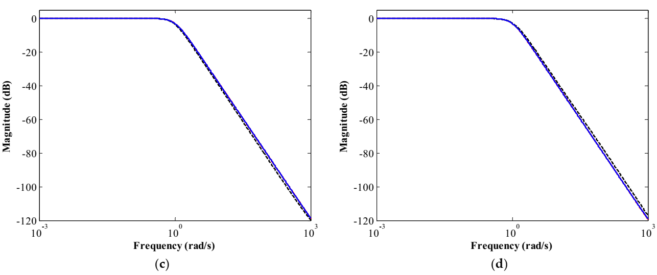
The error function values yielded by the FOLBFs based on the generalized expressions of coefficients for m = 8 and 12 are compared with that of the optimal model in Figure 6. It is found that the function value attained for m = 8 exhibits increased error beyond . Increasing m to 12 results in an error profile nearly similar to the optimal one for up to the 1.82th-order model. The worst accuracy of the generalized FOLBF (m = 12) occurs for . In Figure 7a–d, the magnitude plots of the curve-fitted models for m = 12 are compared with the optimal and the ideal ones for the 1.96–1.99th-order FOLBFs, respectively. For all four cases, although the roll-off behavior of the fitted models remains in proximity to the ideal characteristics, however, the accuracy of these models is slightly inferior when compared against the optimal ones. It may be pointed out that the same modelling errors throughout the entire design range were achieved for the fitted and optimal FOBFs based on the FTF approximation cited in [37,40]. This is due to the small range of variation (between 0 and 2) in the coefficients of the reported optimal FTF models. In contrast, this paper determines the optimal coefficients of the ITF approximant, where the coefficients vary between 0 and 1000. Then, the curve fitting is carried out where the (minimum and maximum) values of the variation for to are (3.2605 × 10⁻⁴, 0.9350), (1.0601, 164.5454), (30.4311, 1339.6233), (31.3957, 1716.1039), (44.0916, 1516.4026), and (30.4168, 1338.3116), respectively. As indicated by the large normr yielded for and it is challenging even for a 12th-degree polynomial approximation to obtain exact matching with the optimal coefficient values.
3.3. Comparison with the Literature
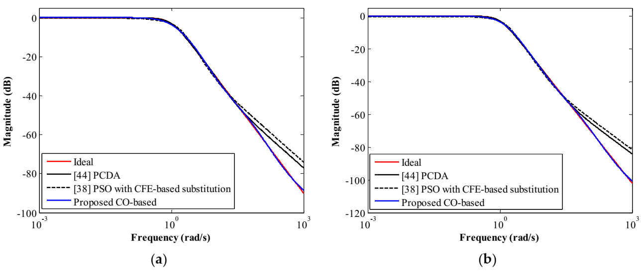
The efficacy of the CO method is demonstrated by comparing with the third-order approximants reported in [38,44]. For demonstration purposes, two arbitrarily chosen models, such as the 1.5th- and the 1.7th-order FOLBFs, are considered. The 1.5th- and 1.7th-order models reported in [38] are given by (27) and (28), respectively; the same for [44] are shown in (29) and (30), respectively.
The magnitude comparison plots for these two design cases are presented in Figure 8a,b. It can be observed that the proposed models achieve good agreement with the theoretical characteristics for six decades of frequency. In contrast, the reported FOLBFs given by (27)–(30) markedly deviates from the ideal response beyond 22.61 Hz, 31.08 Hz, 63.81 Hz, and 55.56 Hz, respectively. Similar results are also found for the other fractional-orders, which are not shown here to avoid redundancy.
3.4. Circuit Realization
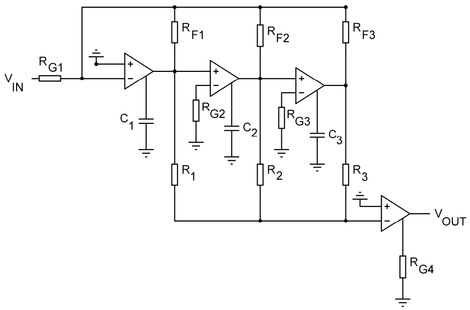
The circuit realization of the proposed rational approximants using the CFOA in follow-the-leader feedback topology is presented in Figure 9. The transfer function of the circuit is given by (31).
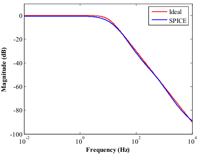
The implementation of the CO-based 1.5th-order model, with a cut-off frequency of 10 Hz, is considered. Since there are 6 design equations and 13 unknown parameters, the following values of components are kept fixed: RG1 = 10 kΩ, RG2 = 10 kΩ, RG3 = 10 kΩ, RG4 = 1 kΩ, RF1 = 1 kΩ, RF2 = 10 kΩ, and R3 = 1 kΩ. The actual values of the other circuit components are derived as follows: R1 = 198.31 kΩ, R2 = 18.59 kΩ, RF3 = 10.12 kΩ, C1 = 224 nF, C2 = 47.87 nF, and C3 = 2.25 uF. For practical purposes, the derived values of components are replaced by the nearest ones from the E96 industrial series as follows: R1 = 200 kΩ, R2 = 18.7 kΩ, RF3 = 10.2 kΩ, C1 = 226 nF, C2 = 47.5 nF, and C3 = 2.26 uF. Simulations are carried out in OrCAD PSPICE with AD844A/AD integrated circuit used as the CFOA. SPICE simulations reveal good agreement to the theoretical magnitude response, as highlighted in Figure 10.
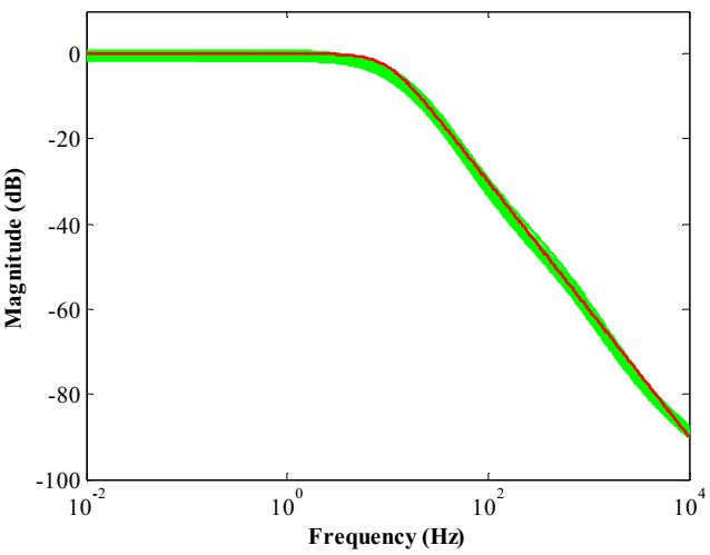
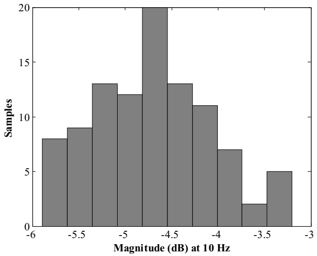
Performance sensitivity to the variations in the passive components is investigated by performing the Monte-Carlo simulations in OrCAD PSPICE. The resistors and capacitors are varied by 5% and 10%, respectively, following the uniform distribution. As demonstrated in Figure 11, the magnitude responses based on 100 Monte-Carlo simulation runs attain proximity to the ideal response throughout the design bandwidth. It is found that the minimum, maximum, mean, and standard deviation indices corresponding to the magnitude at the design cut-off frequency of 10 Hz are −5.890, −3.202, −4.704, and 0.627 dB, respectively. The corresponding Monte-Carlo histogram is shown in Figure 12.
4. Conclusions
A popular technique to obtain an integer-order approximation of a fractional-order filter is to substitute the rational approximant of in the fractional-order transfer function of the filter. The bandwidth of the resultant integer-order model is dependent on the order of the approximated operator. This paper shows that such an integer-order model, when employed as an initial point for a constrained optimization routine, can significantly improve the bandwidth of a FOLBF approximant. The proposed third-order models achieve good agreement with the theoretical magnitude-frequency characteristic over much wider bandwidth (0.001–1000 rad/s) as compared to the state of the art. Future work will investigate the effectiveness of the proposed concept in improving the design bandwidth of the fractional-order generalized filters [55].
Author Contributions
Conceptualization, S.M.; Methodology, S.M.; Software, S.M.; Formal Analysis, S.M.; Investigation, S.M.; Visualization, S.M. and R.K.; Validation, S.M.; Supervision, R.K. and D.M.; Writing—original draft preparation, S.M.; Writing—review & editing, S.M. and R.K. All authors have read and agreed to the published version of the manuscript.
Funding
This research received no external funding.
Acknowledgments
S.M. gratefully acknowledges the fellowship provided by Visvesvaraya PhD Scheme for Electronics & IT, Digital India Corporation, under the Ministry of Electronics & Information Technology, Govt. of India.
Conflicts of Interest
The authors declare no conflict of interest.
Appendix A

Table A1.
Optimal FOLBF models based on the CO method.
| 0.01 | [0.0072, 1.2670, 10.3151, 0.0077, 1.3214, 11.6763, 10.3050] |
| 0.02 | [0.0086, 1.3930, 10.0776, 0.0098, 1.5038, 11.6360, 10.0680] |
| 0.03 | [0.0086, 1.3867, 10.0211, 0.0104, 1.5499, 11.6526, 10.0071] |
| 0.04 | [0.0084, 1.3664, 9.9621, 0.0108, 1.5811, 11.6519, 9.9438] |
| 0.05 | [0.0081, 1.3449, 9.9065, 0.0113, 1.6111, 11.6522, 9.8840] |
| 0.06 | [0.0079, 1.3293, 9.9140, 0.0117, 1.6487, 11.7239, 9.8873] |
| 0.07 | [0.0077, 1.3046, 9.8491, 0.0121, 1.6751, 11.7098, 9.8185] |
| 0.08 | [0.0074, 1.2770, 9.7623, 0.0125, 1.6974, 11.6682, 9.7280] |
| 0.09 | [0.0072, 1.2583, 9.7403, 0.0129, 1.7314, 11.7031, 9.7021] |
| 0.10 | [0.0071, 1.2651, 9.9167, 0.0137, 1.8020, 11.9774, 9.8738] |
| 0.11 | [0.0071, 1.2740, 10.1144, 0.0145, 1.8786, 12.2794, 10.0669] |
| 0.12 | [0.0068, 1.2489, 10.0388, 0.0149, 1.9060, 12.2504, 9.9879] |
| 0.13 | [0.0066, 1.2194, 9.9298, 0.0153, 1.9264, 12.1786, 9.8759] |
| 0.14 | [0.0064, 1.2105, 9.9830, 0.0160, 1.9794, 12.3055, 9.9252] |
| 0.15 | [0.0063, 1.1985, 10.0109, 0.0167, 2.0285, 12.4014, 9.9494] |
| 0.16 | [0.0060, 1.1702, 9.8988, 0.0171, 2.0498, 12.3230, 9.8347] |
| 0.17 | [0.0059, 1.1709, 10.0313, 0.0180, 2.1227, 12.5488, 9.9630] |
| 0.18 | [0.0062, 1.2422, 10.7786, 0.0201, 2.3308, 13.5487, 10.7018] |
| 0.19 | [0.0057, 1.1634, 10.2238, 0.0198, 2.2591, 12.9125, 10.1478] |
| 0.20 | [0.0055, 1.1475, 10.2137, 0.0205, 2.3061, 12.9604, 10.1346] |
| 0.21 | [0.0054, 1.1416, 10.2904, 0.0214, 2.3740, 13.1183, 10.2077] |
| 0.22 | [0.0054, 1.1511, 10.5089, 0.0227, 2.4772, 13.4582, 10.4215] |
| 0.23 | [0.0052, 1.1300, 10.4494, 0.0234, 2.5166, 13.4424, 10.3596] |
| 0.24 | [0.0051, 1.1250, 10.5364, 0.0245, 2.5926, 13.6146, 10.4430] |
| 0.25 | [0.0049, 1.1100, 10.5293, 0.0254, 2.6470, 13.6649, 10.4333] |
| 0.26 | [0.0047, 1.0760, 10.3376, 0.0259, 2.6549, 13.4739, 10.2408] |
| 0.27 | [0.0047, 1.0922, 10.6276, 0.0276, 2.7884, 13.9107, 10.5257] |
| 0.28 | [0.0046, 1.0920, 10.7638, 0.0290, 2.8848, 14.1476, 10.6580] |
| 0.29 | [0.0044, 1.0662, 10.6449, 0.0298, 2.9143, 14.0485, 10.5380] |
| 0.30 | [0.0065, 1.5869, 16.0490, 0.0466, 4.4880, 21.2656, 15.8844] |
| 0.31 | [0.0053, 1.3280, 13.6042, 0.0410, 3.8857, 18.0972, 13.4620] |
| 0.32 | [0.0057, 1.4319, 14.8591, 0.0464, 4.3348, 19.8429, 14.7010] |
| 0.33 | [0.0057, 1.4722, 15.4761, 0.0501, 4.6110, 20.7449, 15.3086] |
| 0.34 | [0.0067, 1.7562, 18.7022, 0.0629, 5.6907, 25.1622, 18.4966] |
| 0.35 | [0.0051, 1.3692, 14.7721, 0.0515, 4.5901, 19.9465, 14.6073] |
| 0.36 | [0.0051, 1.3869, 15.1596, 0.0548, 4.8102, 20.5423, 14.9883] |
| 0.37 | [0.0046, 1.2682, 14.0445, 0.0526, 4.5505, 19.0971, 13.8838] |
| 0.38 | [0.0047, 1.3204, 14.8156, 0.0576, 4.9014, 20.2135, 14.6441] |
| 0.39 | [0.0046, 1.3156, 14.9573, 0.0603, 5.0522, 20.4739, 14.7823] |
| 0.40 | [0.0041, 1.2142, 13.9871, 0.0584, 4.8235, 19.2073, 13.8220] |
| 0.41 | [0.0042, 1.2402, 14.4772, 0.0627, 5.0969, 19.9423, 14.3048] |
| 0.42 | [0.0036, 1.1025, 13.0409, 0.0585, 4.6868, 18.0183, 12.8844] |
| 0.43 | [0.0039, 1.2008, 14.3948, 0.0670, 5.2809, 19.9476, 14.2208] |
| 0.44 | [0.0036, 1.1534, 14.0127, 0.0676, 5.2474, 19.4736, 13.8424] |
| 0.45 | [0.0051, 1.6556, 20.3845, 0.1019, 7.7912, 28.4071, 20.1355] |
| 0.46 | [0.0020, 0.6436, 8.0327, 0.0416, 3.1334, 11.2242, 7.9341] |
| 0.47 | [0.0029, 0.9848, 12.4571, 0.0669, 4.9591, 17.4517, 12.3038] |
| 0.48 | [0.0034, 1.1617, 14.8945, 0.0829, 6.0509, 20.9188, 14.7107] |
| 0.49 | [0.0032, 1.1101, 14.4287, 0.0832, 5.9814, 20.3136, 14.2503] |
| 0.50 | [0.0031, 1.1026, 14.5279, 0.0868, 6.1452, 20.5010, 14.3482] |
| 0.51 | [0.0030, 1.0828, 14.4643, 0.0896, 6.2425, 20.4570, 14.2853] |
| 0.52 | [0.0028, 1.0534, 14.2677, 0.0915, 6.2821, 20.2225, 14.0913] |
| 0.53 | [0.0026, 0.9935, 13.6444, 0.0907, 6.1288, 19.3792, 13.4760] |
| 0.54 | [0.0027, 1.0471, 14.5817, 0.1004, 6.6815, 20.7515, 14.4021] |
| 0.55 | [0.0029, 1.1801, 16.6642, 0.1189, 7.7887, 23.7603, 16.4598] |
| 0.56 | [0.0027, 1.1208, 16.0508, 0.1187, 7.6517, 22.9271, 15.8547] |
| 0.57 | [0.0027, 1.1153, 16.1996, 0.1241, 7.8763, 23.1796, 16.0027] |
| 0.58 | [0.0024, 1.0352, 15.2501, 0.1210, 7.5616, 21.8567, 15.0658] |
| 0.59 | [0.0027, 1.2057, 18.0170, 0.1481, 9.1100, 25.8624, 17.8008] |
| 0.60 | [0.0043, 1.9166, 29.0515, 0.2473, 14.9784, 41.7631, 28.7055] |
| 0.61 | [0.0045, 2.0864, 32.0832, 0.2829, 16.8658, 46.1853, 31.7044] |
| 0.62 | [0.0039, 1.8406, 28.7167, 0.2622, 15.3909, 41.3930, 28.3809] |
| 0.63 | [0.0041, 1.9664, 31.1286, 0.2944, 17.0081, 44.9245, 30.7686] |
| 0.64 | [0.0032, 1.5892, 25.5274, 0.2501, 14.2180, 36.8830, 25.2355] |
| 0.65 | [0.0031, 1.5686, 25.5689, 0.2594, 14.5160, 36.9823, 25.2803] |
| 0.66 | [0.0029, 1.5267, 25.2565, 0.2653, 14.6143, 36.5664, 24.9753] |
| 0.67 | [0.0030, 1.6265, 27.3106, 0.2971, 16.1054, 39.5763, 27.0112] |
| 0.68 | [0.0027, 1.4764, 25.1627, 0.2835, 15.1217, 36.4942, 24.8913] |
| 0.69 | [0.0025, 1.4347, 24.8223, 0.2896, 15.2004, 36.0278, 24.5592] |
| 0.70 | [0.0031, 1.8126, 31.8372, 0.3846, 19.8646, 46.2412, 31.5061] |
| 0.71 | [0.0023, 1.4146, 25.2277, 0.3156, 16.0369, 36.6640, 24.9706] |
| 0.72 | [0.0022, 1.3841, 25.0635, 0.3246, 16.2311, 36.4453, 24.8135] |
| 0.73 | [0.0025, 1.6088, 29.5825, 0.3967, 19.5149, 43.0370, 29.2942] |
| 0.74 | [0.0021, 1.3737, 25.6544, 0.3562, 17.2378, 37.3378, 25.4105] |
| 0.75 | [0.0020, 1.3367, 25.3552, 0.3645, 17.3517, 36.9153, 25.1205] |
| 0.76 | [0.0020, 1.4175, 27.3108, 0.4065, 19.0337, 39.7740, 27.0652] |
| 0.77 | [0.0017, 1.2282, 24.0392, 0.3704, 17.0603, 35.0174, 23.8295] |
| 0.78 | [0.0017, 1.3039, 25.9285, 0.4136, 18.7362, 37.7757, 25.7095] |
| 0.79 | [0.0015, 1.2049, 24.3452, 0.4021, 17.9110, 35.4732, 24.1467] |
| 0.80 | [0.0015, 1.2300, 25.2545, 0.4318, 18.9149, 36.8003, 25.0561] |
| 0.81 | [0.0013, 1.0970, 22.8910, 0.4052, 17.4522, 33.3566, 22.7183] |
| 0.82 | [0.0012, 1.0436, 22.1344, 0.4056, 17.1764, 32.2528, 21.9744] |
| 0.83 | [0.0011, 1.0048, 21.6630, 0.4109, 17.1089, 31.5632, 21.5136] |
| 0.84 | [0.0015, 1.4195, 31.1132, 0.6109, 25.0061, 45.3263, 30.9092] |
| 0.85 | [0.0010, 0.9745, 21.7182, 0.4415, 17.7615, 31.6342, 21.5833] |
| 0.86 | [0.0010, 0.9937, 22.5204, 0.4738, 18.7388, 32.7957, 22.3885] |
| 0.87 | [0.0009, 0.9506, 21.9110, 0.4772, 18.5479, 31.9003, 21.7907] |
| 0.88 | [0.0007, 0.8297, 19.4536, 0.4386, 16.7516, 28.3148, 19.3542] |
| 0.89 | [0.0007, 0.8079, 19.2700, 0.4497, 16.8778, 28.0388, 19.1789] |
| 0.90 | [0.0005, 0.6690, 16.2360, 0.3922, 14.4626, 23.6161, 16.1656] |
| 0.91 | [0.0004, 0.6131, 15.1406, 0.3785, 13.7151, 22.0149, 15.0810] |
| 0.92 | [0.0010, 1.5090, 37.9257, 0.9815, 34.9327, 55.1237, 37.7919] |
| 0.93 | [0.0004, 0.5827, 14.9106, 0.3994, 13.9631, 21.6633, 14.8642] |
| 0.94 | [0.0015, 2.5610, 66.7134, 1.8497, 63.5111, 96.8854, 66.5341] |
| 0.95 | [0.0002, 0.4555, 12.0859, 0.3468, 11.6951, 17.5441, 12.0586] |
| 0.96 | [0.0002, 0.4357, 11.7790, 0.3498, 11.5845, 17.0910, 11.7576] |
| 0.97 | [0.0002, 0.3917, 10.7896, 0.3316, 10.7837, 15.6482, 10.7748] |
| 0.98 | [0.0001, 0.3434, 9.6451, 0.3067, 9.7951, 13.9818, 9.6362] |
| 0.99 | [0.0001, 0.2963, 8.5055, 0.2795, 8.7751, 12.3236, 8.5015] |
References
- Sun, H.G.; Zhang, Y.; Baleanu, D.; Chen, W.; Chen, Y.Q. A new collection of real world applications of fractional calculus in science and engineering. Commun. Nonlinear Sci. Numer. Simul. 2018, 64, 213–231. [Google Scholar] [CrossRef]
- Ortigueira, M.D. An introduction to the fractional continuous-time linear systems: The 21st century systems. IEEE Circuits Syst. Mag. 2008, 8, 19–26. [Google Scholar] [CrossRef] [Green Version]
- Ortiguera, M.D.; Machado, J.A.T. What is a fractional derivative? J. Comput. Phys. 2015, 293, 4–13. [Google Scholar] [CrossRef]
- Matsuda, K.; Fujii, H. H∞—Optimized wave-absorbing control: Analytical and experimental results. J. Guid. Control. Dyn. 1993, 16, 1146–1153. [Google Scholar] [CrossRef]
- Oustaloup, A.; Levron, F.; Mathieu, B.; Nanot, F.; Florence, M. Frequency-band complex noninteger differentiator: Characterization and synthesis. IEEE Trans. Circuits Syst. I Fundam. Theory Appl. 2000, 47, 25–39. [Google Scholar] [CrossRef]
- Xue, D.Y.; Zhao, C.N.; Chen, Y.Q. A modified approximation method of fractional order system. In Proceedings of the 2006 International Conference on Mechatronics and Automation, Luoyang, China, 25–28 June 2006; pp. 1043–1044. [Google Scholar]
- Freeborn, T.J.; Maundy, B.; Elwakil, A. Second-order approximation of the fractional laplacian operator for equal-ripple response. In Proceedings of the 2010 53rd IEEE International Midwest Symposium on Circuits and Systems, Seattle, WA, USA, 1–4 August 2010; pp. 1173–1176. [Google Scholar]
- Krishna, B.T. Studies on fractional order differentiators and integrators: A survey. Signal Process. 2011, 91, 386–426. [Google Scholar] [CrossRef]
- Maundy, B.; Elwakil, A.S.; Freeborn, T.J. On the practical realization of higher-order filters with fractional stepping. Signal Process. 2011, 91, 484–491. [Google Scholar] [CrossRef]
- Gao, Z.; Liao, X. Improved Oustaloup approximation of fractional-order operators using adaptive chaotic particle swarm optimization. J. Syst. Eng. Electron. 2012, 23, 145–153. [Google Scholar] [CrossRef]
- Gao, Z.; Liao, X. Rational approximation for fractional-order system by particle swarm optimization. Nonlinear Dyn. 2012, 67, 1387–1395. [Google Scholar] [CrossRef]
- Valsa, J.; Vlach, J. RC models of a constant phase element. Int. J. Circuit Theory Appl. 2013, 41, 59–61. [Google Scholar] [CrossRef]
- El-Khazali, R. On the biquadratic approximation of fractional-order laplacian operators. Analog. Integr. Circuits Signal Process. 2015, 82, 503–517. [Google Scholar] [CrossRef]
- AbdelAty, A.M.; Elwakil, A.S.; Radwan, A.G.; Psychalinos, C.; Maundy, B.J. Approximation of the fractional-order laplacian sα as a weighted sum of first-order high-pass filters. IEEE Trans. Circuits Syst. II Express Briefs 2018, 65, 1114–1118. [Google Scholar] [CrossRef]
- Yousri, D.; AbdelAty, A.M.; Radwan, A.G.; Elwakil, A.S.; Psychalinos, C. Comprehensive comparison based on meta-heuristic algorithms for approximation of the fractional-order Laplacian sα as a weighted sum of first-order high-pass filters. Microelectron. J. 2019, 87, 110–120. [Google Scholar] [CrossRef]
- Hamed, E.M.; AbdelAty, A.M.; Said, L.A.; Radwan, A.G. Effect of different approximation techniques on fractional-order KHN filter design. Circuits Syst. Signal Process. 2018, 37, 5222–5252. [Google Scholar] [CrossRef]
- Muniz-Montero, C.; Garcia-Jimenez, L.V.; Sanchez-Gaspariano, L.A.; Sanchez-Lopez, C.; Gonzalez-Diaz, V.R.; Tlelo-Cuautle, E. New alternatives for analog implementation of fractional-order integrators, differentiators and PID controllers based on integer-order integrators. Nonlinear Dyn. 2017, 90, 241–256. [Google Scholar] [CrossRef]
- Bertsias, P.; Psychalinos, C.; Elwakil, A.S. Partial fraction expansion based realizations of fractional-order differentiators and integrators using active filters. Int. J. Circuit Theory Appl. 2019, 47, 513–531. [Google Scholar] [CrossRef]
- Kartci, A.; Agambayev, A.; Farhat, M.; Herencsar, N.; Brancik, L.; Bagci, H.; Salama, K.N. Synthesis and optimization of fractional-order elements using a genetic algorithm. IEEE Access 2019, 7, 80233–80246. [Google Scholar] [CrossRef]
- Adhikary, A.; Shil, A.; Biswas, K. Realization of foster structure-based ladder fractor with phase band specification. Circuits Syst. Signal Process. 2020, 39, 2272–2292. [Google Scholar] [CrossRef]
- Kapoulea, S.; Psychalinos, C.; Elwakil, A.S.; Radwan, A.G. One-terminal electronically controlled fractional-order capacitor and inductor emulator. Int. J. Electron. Commun. (AEU) 2019, 103, 32–45. [Google Scholar] [CrossRef]
- Shah, Z.M.; Kathjoo, M.Y.; Khanday, F.A.; Biswas, K.; Psychalinos, C. A survey of single and multi-component fractional-order elements (FOEs) and their applications. Microelectron. J. 2019, 84, 9–25. [Google Scholar] [CrossRef]
- Elwakil, A.S. Fractional-order circuits and systems: An emerging interdisciplinary research area. IEEE Circuits Syst. Mag. 2010, 10, 40–50. [Google Scholar] [CrossRef]
- Freeborn, T.; Maundy, B.; Elwakil, A.S. Approximated fractional order chebyshev lowpass filters. Math. Prob. Eng. 2015, 2015, 832468. [Google Scholar] [CrossRef]
- AbdelAty, A.M.; Soltan, A.; Ahmed, W.A.; Radwan, A.G. On the analysis and design of fractional-order Chebyshev complex filter. Circuits Syst. Signal Process. 2018, 37, 915–938. [Google Scholar] [CrossRef]
- Freeborn, T.; Elwakil, A.S.; Maundy, B. Approximated fractional-order inverse chebyshev lowpass filters. Circuits Syst. Signal Process. 2016, 35, 1973–1982. [Google Scholar] [CrossRef]
- Freeborn, T.J.; Kubanek, D.; Koton, J.; Dvorak, J. Validation of fractional-order lowpass elliptic responses of (1+α)-order analog filters. Appl. Sci. 2018, 8, 1–17. [Google Scholar]
- Said, L.A.; Ismail, S.M.; Radwan, A.G.; Madian, A.H.; El-Yazeed, M.F.A.; Soliman, A.M. On the optimization of fractional order low-pass filters. Circuits Syst. Signal Process. 2016, 35, 2017–2039. [Google Scholar] [CrossRef]
- Ahmadi, P.; Maundy, B.; Elwakil, A.S.; Belostotski, L. High-quality factor asymmetric-slope band-pass filters: A fractional-order capacitor approach. IET Circuits Devices Syst. 2012, 6, 187–198. [Google Scholar] [CrossRef]
- Kubanek, D.; Freeborn, T.; Koton, J. Fractional-order band-pass filter design using fractional-characteristic specimen functions. Microelectron. J. 2019, 86, 77–86. [Google Scholar] [CrossRef]
- Baranowski, J.; Pauluk, M.; Tutaj, A. Analog realization of fractional filters: Laguerre approximation approach. Int. J. Electron. Commun. (AEU) 2018, 81, 1–11. [Google Scholar] [CrossRef]
- Adhikary, A.; Sen, S.; Biswas, K. Practical realization of tunable fractional order parallel resonator and fractional order filters. IEEE Trans Circuits Syst. I 2016, 63, 1142–1151. [Google Scholar] [CrossRef]
- Mahata, S.; Saha, S.K.; Kar, R.; Mandal, D. Approximation of fractional-order low pass filter. IET Signal Process. 2019, 13, 112–124. [Google Scholar] [CrossRef]
- Mahata, S.; Saha, S.; Kar, R.; Mandal, D. Optimal integer-order rational approximation of α and α+β fractional-order generalised analogue filters. IET Signal Process. 2019, 13, 516–527. [Google Scholar] [CrossRef]
- Ali, A.S.; Radwan, A.G.; Soliman, A.M. Fractional order butterworth filter: Active and passive realizations. IEEE J. Emerg. Sel. Top. Circuits Syst. 2013, 3, 346–354. [Google Scholar] [CrossRef]
- Acharya, A.; Das, S.; Pan, I.; Das, S. Extending the concept of analog butterworth filter for fractional order systems. Signal Process. 2014, 94, 409–420. [Google Scholar] [CrossRef] [Green Version]
- Freeborn, T.J. Comparison of (1+α) fractional-order transfer functions to approximate lowpass butterworth magnitude responses. Circuits Syst. Signal Process. 2016, 35, 1983–2002. [Google Scholar] [CrossRef]
- Singh, N.; Mehta, U.; Kothari, K.; Cirrincione, M. Optimized fractional low and highpass filters of (1+α) order on FPAA. Bull. Pol. Acad. Sci. 2020, 68, 635–644. [Google Scholar]
- Kubanek, D.; Freeborn, T.; Koton, J.; Herencsar, N. Evaluation of (1+α) fractional-order approximated butterworth high-pass and band-pass filter transfer functions. Elektron. Elektrotechnika 2018, 24, 37–41. [Google Scholar] [CrossRef] [Green Version]
- Mahata, S.; Kar, R.; Mandal, D. Optimal fractional-order highpass Butterworth magnitude characteristics realization using current-mode filter. Int. J. Electron. Commun. (AEU) 2019, 102, 78–89. [Google Scholar] [CrossRef]
- Psychalinos, C.; Tsirimokou, G.; Elwakil, A.S. Switched-capacitor fractional-step butterworth filter design. Circuits Syst. Signal Process. 2016, 35, 1377–1393. [Google Scholar] [CrossRef]
- Freeborn, T.J.; Maundy, B.; Elwakil, A.S. Field programmable analogue array implementation of fractional step filters. IET Circuits Devices Syst. 2010, 4, 514–524. [Google Scholar] [CrossRef]
- Mahata, S.; Saha, S.K.; Kar, R.; Mandal, D. Optimal design of fractional order low pass Butterworth filter with accurate magnitude response. Digit. Signal Process. 2018, 72, 96–114. [Google Scholar] [CrossRef]
- Mahata, S.; Banerjee, S.; Kar, R.; Mandal, D. Revisiting the use of squared magnitude function for the optimal approximation of (1+α) order Butterworth filter. Int. J. Electron. Commun. (AEU) 2019, 110, 152826. [Google Scholar] [CrossRef]
- Mahata, S.; Saha, S.K.; Kar, R.; Mandal, D. Accurate integer order rational approximation of fractional order low pass Butterworth filter using a metaheuristic optimization approach. IET Signal Process. 2018, 12, 581–589. [Google Scholar] [CrossRef]
- Mahata, S.; Kar, R.; Mandal, D. Comparative study of nature-inspired algorithms to design (1+α) and (2+α)-order filters using a frequency-domain approach. Swarm Evol. Comput. 2020, 55, 100685. [Google Scholar] [CrossRef]
- Mahata, S.; Kar, R.; Mandal, D. Optimal rational approximation of bandpass Butterworth filter with symmetric fractional-order roll-off. Int. J. Electron. Commun. (AEU) 2020, 117, 153106. [Google Scholar] [CrossRef]
- Mahata, S.; Kar, R.; Mandal, D. Optimal approximation of asymmetric type fractional-order bandpass Butterworth filter using decomposition technique. Int. J. Circuit Theory Appl. 2020, 48, 1554–1560. [Google Scholar] [CrossRef]
- Mahata, S.; Kar, R.; Mandal, D. Direct digital fractional-order Butterworth filter design using constrained optimization. Int. J. Electron. Commun. (AEU) 2020, 128, 153511. [Google Scholar] [CrossRef]
- Mahata, S.; Kar, R.; Mandal, D. Optimal design of lattice wave digital fractional-order Butterworth filter. Int. J. Circuit Theory Appl. 2020. [Google Scholar] [CrossRef]
- Soliman, A.M. Applications of the current feedback operational amplifiers. Analog. Integr. Circuits Signal Process. 1996, 11, 265–302. [Google Scholar] [CrossRef]
- Tsirimokou, G.; Koumousi, S.; Psychalinos, C. Design of fractional-order filters using current feedback operational amplifiers. J. Eng. Sci. Technol. Rev. 2016, 9, 77–81. [Google Scholar] [CrossRef]
- Mahata, S.; Kar, R.; Mandal, D. Optimal approximation of fractional-order systems with model validation using CFOA. IET Signal Process. 2019, 13, 787–797. [Google Scholar] [CrossRef]
- Ogata, K. System Dynamics, 4th ed.; Pearson Prentice Hall: Upper Saddle River, NJ, USA, 2004. [Google Scholar]
- Tsirimokou, G.; Psychalinos, C.; Elwakil, A.S. Fractional-order electronically controlled generalized filters. Int. J. Circuit Theory Appl. 2017, 45, 595–612. [Google Scholar] [CrossRef]
Figure 1.
Comparison of error fitness values for the designed FOLBFs based on the pole-zero optimization with (14) (black circle), pole-zero optimization with (15) (blue pentagon), and the constrained optimization technique (red square).
Figure 1.
Comparison of error fitness values for the designed FOLBFs based on the pole-zero optimization with (14) (black circle), pole-zero optimization with (15) (blue pentagon), and the constrained optimization technique (red square).

Figure 2.
Comparison plots for the 1.2nd-order FOLBFs before and after optimization regarding the (a) magnitude, and (b) phase.
Figure 2.
Comparison plots for the 1.2nd-order FOLBFs before and after optimization regarding the (a) magnitude, and (b) phase.

Figure 3.
Comparison plots for the 1.5th-order FOLBFs before and after optimization regarding the (a) magnitude, and (b) phase.
Figure 3.
Comparison plots for the 1.5th-order FOLBFs before and after optimization regarding the (a) magnitude, and (b) phase.

Figure 4.
Comparison plots for the 1.8th-order FOLBFs before and after optimization regarding the (a) magnitude, and (b) phase.
Figure 4.
Comparison plots for the 1.8th-order FOLBFs before and after optimization regarding the (a) magnitude, and (b) phase.

Figure 5.
Comparison of execution time for the designed FOLBFs based on the pole-zero optimization with (14) (black circle), pole-zero optimization with (15) (blue pentagon), and the constrained optimization technique (red square).
Figure 5.
Comparison of execution time for the designed FOLBFs based on the pole-zero optimization with (14) (black circle), pole-zero optimization with (15) (blue pentagon), and the constrained optimization technique (red square).

Figure 6.
Comparison of function values between the optimal and curve-fitted FOLBFs.

Figure 7.
Magnitude comparison plots for the curve-fitted (m = 12) models (dashed black) with the optimal (solid blue) and ideal FOLBFs (solid red) for α of (a) 0.96, (b) 0.97, (c) 0.98, and (d) 0.99.
Figure 7.
Magnitude comparison plots for the curve-fitted (m = 12) models (dashed black) with the optimal (solid blue) and ideal FOLBFs (solid red) for α of (a) 0.96, (b) 0.97, (c) 0.98, and (d) 0.99.


Figure 8.
Magnitude response comparison plots with the cited literature for the (1+α)-order FOLBFs with α of (a) 0.50, and (b) 0.70.
Figure 8.
Magnitude response comparison plots with the cited literature for the (1+α)-order FOLBFs with α of (a) 0.50, and (b) 0.70.

Figure 9.
CFOA-based circuit realization of the proposed FOLBF.

Figure 10.
SPICE simulated magnitude-frequency plot for the CO-based 1.5th-order FOLBF.

Figure 11.
Magnitude response of the CO-based 1.5th-order FOLBF based on Monte-Carlo simulations (green) as compared to the theoretical characteristic (red).
Figure 11.
Magnitude response of the CO-based 1.5th-order FOLBF based on Monte-Carlo simulations (green) as compared to the theoretical characteristic (red).

Figure 12.
Monte-Carlo histogram for the magnitude of the CO-based 1.5th-order FOLBF at the cut-off frequency.
Figure 12.
Monte-Carlo histogram for the magnitude of the CO-based 1.5th-order FOLBF at the cut-off frequency.

Table 1.
Coefficients of the polynomial based on (26) for m = 12 and the norm of residuals.
| j | normr | |
|---|---|---|
| 1 | [−3296.4822 20,463.0535 −55,956.3172 88,645.9592 −90,004.6700 61,177.1067 −28,220.1541 8748.7235 −1744.8383 188.7039 3.8243 −5.9044 0.9941] | 0.0121 |
| 2 | [5,360,719.0307 −33,661,093.4010 93,344,686.5258 −150,459,613.8980 156,126,064.8060 −109,126,929.1226 52,244,368.4342 −17,082,989.8734 3,738,541.4525 −526,969.6843 45,711.4164 −2677.7164 184.9341] | 5.5319 |
| 3 | [98,181,518.8867 −616,171,022.1666 1,707,614,135.6472 −2,750,396,416.1026 2,851,379,332.7390 −1,990,736,903.7900 951,625,592.6166 −310,495,794.2945 67,704,359.2792 −9,459,845.1519 791,119.5979 −37,614.9184 1602.1394] | 102.8524 |
| 4 | [5,655,736.7928 −35,483,357.2034 98,304,655.4191 −158,285,807.3359 164,049,687.1309 −114,509,031.6440 54,735,501.9212 −17,864,163.7748 3,898,895.3782 −545,744.8998 45,696.4819 −2222.8002 187.4012] | 5.7409 |
| 5 | [104,678,306.0497 −656,934,043.5111 1,820,552,445.4560 −2,932,252,271.2739 3,039,861,753.9281 −2,122,300,914.9943 1,014,512,284.2268 −331,018,580.3175 72,181,180.2320 −10,084,151.3121 842,086.1104 −39,808.1889 1793.5872] | 109.4323 |
| 6 | [97,902,861.1308 −614,425,103.7567 1,702,785,070.0630 −2,742,636,550.9125 2,843,357,267.3012 −1,985,155,645.3550 948,969,406.0082 −309,634,398.9421 67,518,446.8187 −9,434,553.4453 789,240.7331 −37,575.9960 1600.7331] | 102.5444 |
Publisher’s Note: MDPI stays neutral with regard to jurisdictional claims in published maps and institutional affiliations. |
© 2020 by the authors. Licensee MDPI, Basel, Switzerland. This article is an open access article distributed under the terms and conditions of the Creative Commons Attribution (CC BY) license (http://creativecommons.org/licenses/by/4.0/).
Share and Cite
MDPI and ACS Style
Mahata, S.; Kar, R.; Mandal, D. Optimal Modelling of (1 + α) Order Butterworth Filter under the CFE Framework. Fractal Fract. 2020, 4, 55. https://0-doi-org.brum.beds.ac.uk/10.3390/fractalfract4040055
AMA Style
Mahata S, Kar R, Mandal D. Optimal Modelling of (1 + α) Order Butterworth Filter under the CFE Framework. Fractal and Fractional. 2020; 4(4):55. https://0-doi-org.brum.beds.ac.uk/10.3390/fractalfract4040055
Chicago/Turabian StyleMahata, Shibendu, Rajib Kar, and Durbadal Mandal. 2020. "Optimal Modelling of (1 + α) Order Butterworth Filter under the CFE Framework" Fractal and Fractional 4, no. 4: 55. https://0-doi-org.brum.beds.ac.uk/10.3390/fractalfract4040055