Fractional-Fractal Modeling of Filtration-Consolidation Processes in Saline Saturated Soils

Abstract

To study the peculiarities of anomalous consolidation processes in saturated porous (soil) media in the conditions of salt transfer, we present a new mathematical model developed on the base of the fractional-fractal approach that allows considering temporal non-locality of transfer processes in media of fractal structure. For the case of the finite thickness domain with permeable boundaries, a finite-difference technique for numerical solution of the corresponding one-dimensional non-linear boundary value problem is developed. The paper also presents a fractional-fractal model of a filtration-consolidation process in clay soils of fractal structure saturated with salt solutions. An analytical solution is found for the corresponding one-dimensional boundary value problem in the domain of finite thickness with permeable upper and impermeable lower boundaries.

1. Introduction

The determination of the conditions for the safe functioning of industrial and domestic wastewater storage facilities, as well as numerous other engineering facilities that pollute soils and groundwater, are among the most important and relevant, primarily in the connection with environment protection issues. This makes urgent the development of effective and reliable methods for mathematical modeling of deformation and compaction (consolidation) dynamics in saturated soils, particularly, in the foundations of hydraulic structures. Theoretical studies of the peculiarities of filtration-consolidation dynamics in porous media are often reduced to the solution of boundary value problems for the corresponding systems of partial differential or integro-differential equations [1,2,3,4,5,6,7,8]. In recent decades, a number of mathematical models in fractional-differential formulation have been developed to study the features of anomalous consolidation processes taking into account memory effects and spatial correlations [9,10,11,12].

In this paper, to simulate anomalous dynamics of filtration-consolidation processes in saturated porous (soil) media in the conditions of salt transfer we use the fractional-fractal approach [13,14,15] that allows taking into account temporal non-locality of processes in soils of fractal structure in the corresponding mathematical models. We combine the space-fractal advection-dispersion equation introduced in Reference [13] with time-fractional filtration-consolidation model studied in References [10,12] obtaining a new fractional-fractal model of an anomalous process of filtration-consolidation in a compacting soil of fractal structure. Comparing to the model studied in Reference [13], the presented model is time-fractional and contains an equation for determining a velocity field taking chemical osmosis [16,17] into account. For this new model we pose an initial-boundary value problem and present a finite-difference technique for its numerical solution. We also obtain an exact solution of a similar model that is considered in the case when ultrafiltration phenomenon [17] is taken into account but advection term can be neglected.

2. Fractional-Fractal Mathematical Model of Filtration-Consolidation Processes in Saline Saturated Soils

Considering a non-local in time isothermal filtration-consolidation process in a soil of fractal structure saturated with a salt solution, we start from the following generalizations of the Darcy’s and Fick’s laws:

$$u_x=D_t^{1-\beta }\frac{\partial }{\partial x^{\alpha }}\left(-kH+\nu C\right),$$

(1)

$$q_c=D_t^{1-\beta }\left(-d_{*}\frac{\partial C}{\partial x^{\alpha }}+C{J}_t^{1-\beta }{u}_x\right),$$

(2)

where $u_x$ is the filtration rate, $H(x,t)=p/\gamma$ is the water head, p is the pore pressure, $\gamma$ is the liquid density, $C(x,t)$ is the concentration of salts in the liquid phase, k is the filtration coefficient, $\nu$ is the coefficient of chemical osmosis [2], $q_c$ is the diffusion flow, $d_{*}$ is the coefficient of convective diffusion [18], $J_t^{1-\beta }f\left(t\right)=\frac{1}{\mathsf{\Gamma }(1-\beta )}{\int }_0^t{(t-\tau )}^{-\beta }f\left(\tau \right)d\tau$ is the fractional Riemann-Liouville integral of order $1-\beta$, $0<\beta \le 1$, $D_t^{1-\beta }f\left(t\right)=\frac{d}{dt}{J}_t^{\beta }$ is the operator of Riemann-Liouville fractional differentiation of the same order with respect to the variable t [19,20,21], $\frac{\partial }{\partial x^{\alpha }}f\left(x\right)={\displaystyle \underset{x_1\to x}{lim}}\frac{f\left(x\right)-f\left(x_1\right)}{x^{\alpha }-x_1^{\alpha }}$ is the operator of the fractal derivative [13,14,15], $\alpha >0$ is the fractal dimension.

The Equations (1) and (2) are obtained combining fractal-fractional generalizations of the corresponding laws presented in Reference [14] and an approach for taking chemical osmosis into account described in Reference [16].

Following the classical soil consolidation theory of V.A. Florin [5,8] we consider an approximation of porosity change in the form $\frac{\partial n}{\partial t}\approx \frac{1}{1+\widehat{e}}\frac{\partial e}{\partial t}$ where n is the porosity of the medium, e is the coefficient of porosity, $\widehat{e}$ is its average value. Further we use a generalized equation of filtration flow continuity [14] for the case of fractal-structured media in the form $\frac{\partial n}{\partial t}=\frac{\partial u_x}{\partial x^{\alpha }}$. Assuming [5,8] that changes in porosity coefficient depend only on the sum of principal stresses and the strain-stress state of soil depends only on hydraulic pressure, we obtain the following form of a linear law of compaction:

$$\frac{\partial u_x}{\partial x^{\alpha }}+\frac{k}{C_{\upsilon }}\frac{\partial H}{\partial t}=0$$

(3)

Substituting Equation (1) into Equation (3) we get the equation for water head in the form

$$D_t^{\left(\beta \right)}H=\frac{\partial }{\partial x^{\alpha }}\left(\frac{\partial }{\partial x^{\alpha }}\left(C_{\upsilon }H-\mu C\right)\right),$$

(4)

where $C_{\upsilon }$ is the consolidation coefficient [5,6,7,8], $\mu =\frac{\nu C_{\upsilon }}{k}$, $D_t^{\left(\beta \right)}f\left(t\right)=\frac{1}{\mathsf{\Gamma }(1-\beta )}\frac{\partial }{\partial t}\left({\int }_0^t{(t-\tau )}^{-\beta }f\left(\tau \right)d\tau -{\tau }^{-\beta }f\left(0\right)\right)$ is the operator of the regularized fractional Caputo-Gerasimov derivative of the order $\beta$ with respect to the variable t [19,20,21]. The usage of the regularized derivative is here motivated by the known restrictions on initial conditions imposed in the case then the non-regularized derivative is used [22,23]

From the generalized balance equation for salts in the liquid phase in a soil of fractal structure, taking Equation (2) into account we obtain an equation for determination of salts concentration in groundwater flow in the form

$$\sigma D_t^{\left(\beta \right)}C=d_{*}\frac{\partial }{\partial x^{\alpha }}\left(\frac{\partial C}{\partial x^{\alpha }}\right)+\frac{\partial }{\partial x^{\alpha }}\left(kH-\nu C\right)·\frac{\partial C}{\partial x^{\alpha }},$$

(5)

where $\sigma$ is the porosity of the medium [18].

From Equations (4) and (5) when $\alpha \to 1$ we obtain a system of equations [24] of the fractional-differential model of filtration-consolidation in a soil saturated with a salt solution without considering its fractal properties. When $\alpha ,\beta \to 1$ the system (4) and (5) becomes reduced to the following well-known system of equations in the classical formulation [1,2]:

$$\frac{\partial H}{\partial t}=\frac{{\partial }^2}{\partial x^2}\left(C_{\upsilon }H-\mu C\right),$$

$$\sigma \frac{\partial C}{\partial t}=d_{*}\frac{{\partial }^{2}C}{\partial x^2}+\frac{\partial }{\partial x}\left(kH-\nu C\right)·\frac{\partial C}{\partial x}.$$

Using the representation of fractal derivative operator through integer-order derivative in the form $\frac{d}{d{x}^{\alpha }}f\left(x\right)=\frac{d}{dx}f\left(x\right)\frac{1}{\alpha x^{\alpha -1}}$ [13,14,15] in Equations (4) and (5) and reducing similar terms, we obtain the model’s system of equations in the following form:

$$D_t^{\left(\beta \right)}H=C_{\upsilon }\left[s_{\alpha }\left(x\right)\frac{{\partial }^{2}H}{\partial x^2}+r_{\alpha }\left(x\right)\frac{\partial H}{\partial x}\right]-\mu \left[s_{\alpha }\left(x\right)\frac{{\partial }^{2}C}{\partial x^2}+r_{\alpha }\left(x\right)\frac{\partial C}{\partial x}\right],$$

(6)

$$\sigma D_t^{\left(\beta \right)}C=d_{*}\left[s_{\alpha }\left(x\right)\frac{{\partial }^{2}C}{\partial x^2}+r_{\alpha }\left(x\right)\frac{\partial C}{\partial x}\right]+s_{\alpha }\left(x\right)\frac{\partial \upsilon }{\partial x}·\frac{\partial C}{\partial x}$$

(7)

where

$$\upsilon (x,t)=kH(x,t)-\nu C(x,t),r_{\alpha }\left(x\right)=\frac{1-\alpha }{{\alpha }^2}{x}^{1-2\alpha },s_{\alpha }\left(x\right)=\frac{1}{{\alpha }^2}{x}^{2(1-\alpha )}.$$

Within the framework of such non-classical mathematical model, the fractional-differential dynamics of a non-local in time filtration-consolidation process in a soil of fractal structure saturated with a salt solution in the case of the domain of finite thickness l with permeable boundaries is described in the domain $\mathsf{\Omega }=\left\{(x,t):0<x<l,t>0\right\}$ by the system of Equations (6) and (7) with the following boundary conditions:

$$H(0,t)=0,H(l,t)=0,H(x,0)=H_0,$$

(8)

$$C(0,t)=C_0,C(l,t)=0,C(x,0)=0,$$

(9)

where $H_0$ is the initial value of water head, $C_0$ is the value of salts concentration at the inlet of the filtration flow.

3. Numerical Modeling of Fractional-Differential Consolidation Dynamics of a Saline Saturated Soil Massif of Finite Thickness and Fractal Structure

Below we present a brief summary of a finite-difference technique for constructing an approximate solution of the non-linear boundary value problem (6)–(9).

We define the grid domain

$${\omega }_{h\tau }=\left\{(x_i,t_j):x_i=ih(i=\overline{0,m+1}),t_j=j\tau (j=\overline{0,n}),\right\}$$

where $h,\tau$ are the grid steps with respect to the geometric variable and time, and discretize the considered problem at the time step $t_{j+1}$ and in the point $x_i$, $C=C_i^{j+1}=C(x_i,t_{j+1})$, $\widehat{C}=C_i^j$ using the linearized Crank–Nicholson scheme as

$$\sigma {\Delta }_t^{\left(\beta \right)}C=0.5d_{*}\left[s_{\alpha }\left({\widehat{C}}_{\overline{x}x}+C_{\overline{x}x}\right)+r_{\alpha }\left({\widehat{C}}_{\stackrel{0}{x}}+C_{\stackrel{0}{x}}\right)\right]+0.5s_{\alpha }{\upsilon }_{\stackrel{0}{x}}\left({\widehat{C}}_{\stackrel{0}{x}}+C_{\stackrel{0}{x}}\right),$$

(10)

$$\begin{array}{c}{\Delta }_t^{\left(\beta \right)}H=0.5C_{\upsilon }\left[s_{\alpha }\left({\widehat{H}}_{\overline{x}x}+H_{\overline{x}x}\right)+r_{\alpha }\left({\widehat{H}}_{\stackrel{0}{x}}+H_{\stackrel{0}{x}}\right)\right]-\hfill \\ -0.5\mu \left[s_{\alpha }\left({\widehat{C}}_{\overline{x}x}+C_{\overline{x}x}\right)+r_{\alpha }\left({\widehat{C}}_{\stackrel{0}{x}}+C_{\stackrel{0}{x}}\right)\right]\hfill \end{array},$$

(11)

where [25] $C_{\overline{x}x}=\frac{1}{h^2}(C_{i-1}-2C_i+C_{i+1})$, $C_{\stackrel{0}{x}}=\frac{1}{h}(C_{i+1}-C_{i-1})$ and the same notations are used for H.

The operator ${\Delta }_t^{\left(\beta \right)}u$ denotes a discrete analogue of the Caputo-Gerasimov fractional derivative $D_t^{\left(\beta \right)}u$ and is defined as

$${\Delta }_{t_{j+1}}^{\left(\beta \right)}u\approx \frac{u^{j+1}-u^j}{{\tau }^{\beta }\mathsf{\Gamma }(2-\beta )}+\sum _{v=0}^{j-1}{\omega }_v^{\left(j\right)}\frac{u^{v+1}-u^v}{\tau },$$

(12)

${\omega }_v^{\left(j\right)}=\frac{{\tau }^{1-\beta }}{\mathsf{\Gamma }(2-\beta )}\left[{(j-v+1)}^{1-\beta }-{(j-v)}^{1-\beta }\right]$, $\mathsf{\Gamma }\left(z\right)$ is the Euler’s gamma function [26,27]. Let us note that in the class of sufficiently smooth functions we have $D_t^{\left(\beta \right)}u={\Delta }_t^{\left(\beta \right)}u+O\left(\tau \right)$ [19,20,21].

Taking Equation (12) into account in Equations (10) and (11) we reduce the solution of the considered problem at the $(j+1)$-th time step to the solution of the following systems of linear algebraic equations:

$$A_i^j{C}_{i-1}^{j+1}-S_i^j{C}_i^{j+1}+B_i^j{C}_{i+1}^{j+1}=F_i^j(i=\overline{1,m};j=\overline{0,n}),$$

(13)

$${\tilde{A}}_i^j{H}_{i-1}^{j+1}-{\tilde{S}}_i^j{H}_i^{j+1}+{\tilde{B}}_i^j{H}_{i+1}^{j+1}={\tilde{F}}_i^j(i=\overline{1,m};j=\overline{0,n}),$$

(14)

$$C_0^{j+1}=C_0,C_{m+1}^{j+1}=0,C_i^0=0(i=\overline{0,m+1};j=\overline{0,n}),$$

(15)

$$H_0^{j+1}=0,H_{m+1}^{j+1}=0,H_i^0=H_0(i=\overline{0,m+1};j=\overline{0,n}),$$

(16)

where

$$A_i^j=\frac{0.5}{h}\left[d_{*}\left(\frac{s_{\alpha }^i}{h}-\frac{r_{\alpha }^i}{2}\right)-\frac{s_{\alpha }^i}{4h}\left({\upsilon }_{i+1}^j-{\upsilon }_{i-1}^j\right)\right],B_i^j=\frac{0.5}{h}\left[d_{*}\left(\frac{s_{\alpha }^i}{h}+\frac{r_{\alpha }^i}{2}\right)+\frac{s_{\alpha }^i}{4h}\left({\upsilon }_{i+1}^j-{\upsilon }_{i-1}^j\right)\right],$$

$$S_i^j=A_i^j+B_i^j+\frac{\sigma }{{\tau }^{\beta }\mathsf{\Gamma }(2-\beta )},$$

$$\begin{array}{c}{F}_i^j=\sigma \left[\sum _{v=0}^{j-1}{\omega }_v^{\left(j\right)}\frac{C_i^{v+1}-C_i^v}{\tau }-\frac{C_i^j}{{\tau }^{\beta }\mathsf{\Gamma }(2-\beta )}\right]-\frac{0.5d_{*}}{h}\left[\frac{s_{\alpha }^i}{h}\left(C_{i-1}^j-2C_i^j+C_{i+1}^j\right)+\frac{r_{\alpha }^i}{2}\left(C_{i+1}^j-C_{i-1}^j\right)\right]-\hfill \\ -\frac{0.5s_{\alpha }^i}{4h^2}\left({\upsilon }_{i+1}^j-{\upsilon }_{i-1}^j\right)\left(C_{i+1}^j-C_{i-1}^j\right),\hfill \end{array}$$

$${\tilde{A}}_i^j=\frac{0.5C_{\upsilon }}{h}\left(\frac{s_{\alpha }^i}{h}-\frac{r_{\alpha }^i}{2}\right),{\tilde{B}}_i^j=\frac{0.5C_{\upsilon }}{h}\left(\frac{s_{\alpha }^i}{h}+\frac{r_{\alpha }^i}{2}\right),{\tilde{S}}_i^j={\tilde{A}}_i^j+{\tilde{B}}_i^j+\frac{1}{{\tau }^{\beta }\mathsf{\Gamma }(2-\beta )},$$

$$\begin{array}{c}{\tilde{F}}_i^j=\sum _{v=0}^{j-1}{\omega }_v^{\left(j\right)}\frac{H_i^{v+1}-H_i^v}{\tau }-\frac{H_i^j}{{\tau }^{\beta }\mathsf{\Gamma }(2-\beta )}-\frac{0.5C_{\upsilon }}{h}\left[\frac{s_{\alpha }^i}{h}\left(H_{i-1}^j-2H_i^j+H_{i+1}^j\right)+\frac{r_{\alpha }^i}{2}\left(H_{i+1}^j-H_{i-1}^j\right)\right]+\hfill \\ +\frac{0.5\mu }{h}\left[\frac{s_{\alpha }^i}{h}\left(C_{i-1}^{j+1}-2C_i^{j+1}+C_{i+1}^{j+1}+C_{i-1}^j-2C_i^j+C_{i+1}^j\right)+\frac{r_{\alpha }^i}{2}\left(C_{i+1}^{j+1}-C_{i-1}^{j+1}+C_{i+1}^j-C_{i-1}^j\right)\right],\hfill \end{array}$$

$$s_{\alpha }^i=s_{\alpha }\left(x_i\right),r_{\alpha }^i=r_{\alpha }\left(x_i\right),{\upsilon }_i^j=k{H}_i^j-\nu C_i^j.$$

The sums in $F_i^j,{\tilde{F}}_i^j$ are here considered to be equal to zero when $j=0$.

Difference Equations (13) and (14) are three-point and can be effectively solved by the Thomas algorithm [25] as follows:

$$C_i^{j+1}={\tilde{\xi }}_{i+1}^j{C}_{i+1}^{j+1}+{\tilde{\zeta }}_{i+1}^j,H_i^{j+1}={\xi }_{i+1}^j{H}_{i+1}^{j+1}+{\zeta }_{i+1}^j(i=\overline{1,m};j=\overline{0,n}),$$

$${\tilde{\xi }}_{i+1}^j=\frac{B_i^j}{S_i^j-A_i^j{\tilde{\xi }}_i^j},{\tilde{\zeta }}_{i+1}^j=\frac{{\tilde{\xi }}_{i+1}^j}{B_i^j}\left(A_i^j{\tilde{\zeta }}_i^j-F_i^j\right)(i=\overline{1,m};j=\overline{0,n}),$$

$${\xi }_{i+1}^j=\frac{{\tilde{B}}_i^j}{{\tilde{S}}_i^j-{\tilde{A}}_i^j{\xi }_i^j},{\zeta }_{i+1}^j=\frac{{\xi }_{i+1}^j}{{\tilde{B}}_i^j}\left({\tilde{A}}_i^j{\zeta }_i^j-{\tilde{F}}_i^j\right)(i=\overline{1,m};j=\overline{0,n}).$$

To determine the starting values of the coefficients, we use finite-difference analogues of the boundary conditions (15) and (16) obtaining

$${\tilde{\xi }}_1^j=0,{\tilde{\zeta }}_1^j=C_0,{\xi }_1^j=0,{\zeta }_1^j=0(j=\overline{0,n}).$$

Recalling that the Thomas algorithm is stable when linear system’s matrix is diagonally dominant [25], we can state that it is stable for the systems (13) and (14) for such existing values of $\tau \left(h\right)$ that $|S_i^j|>|A_i^j|$ and $|S_i^j|>|B_i^j|$.

4. Results of Numerical Experiments on Modeling the Dynamics of the Consolidation Process

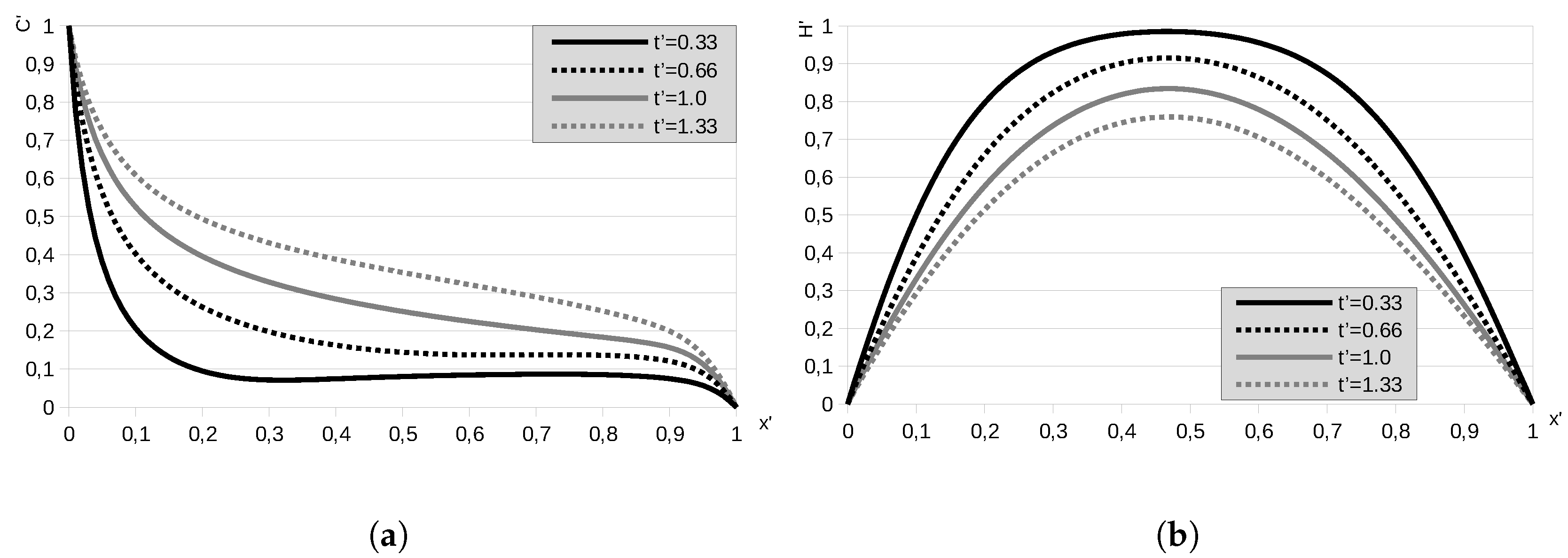
Numerical modeling of the dynamics of water head and concentration fields according to the presented mathematical model was performed for input data from Reference [2]. Some results obtained with respect to the dimensionless variables $x^{\prime }=\frac{x}{x_0}$, $t^{\prime }=\frac{t}{t_0}$, $C^{\prime }=\frac{C}{C_0}$, $H^{\prime }=\frac{H}{H_0}$ are shown in Figure 1, Figure 2 and Figure 3. Here $C_0=200$ g/L, $H_0=10$ m, $x_0=25$ m, $t_0=60$ days.

The analysis of numerical experiments’ results allows us to draw the following conclusions:

• The general tendencies in the distribution of concentration and water head fields in the consolidating soil massif modeled within the framework of the presented fractional-fractal model is generally in concordance with the tendencies in the distribution of similar fields obtained using the fractional-differential model [9,24] that takes into account memory effects, but not fractal properties of the medium, as well as with the classical consolidation model [2].
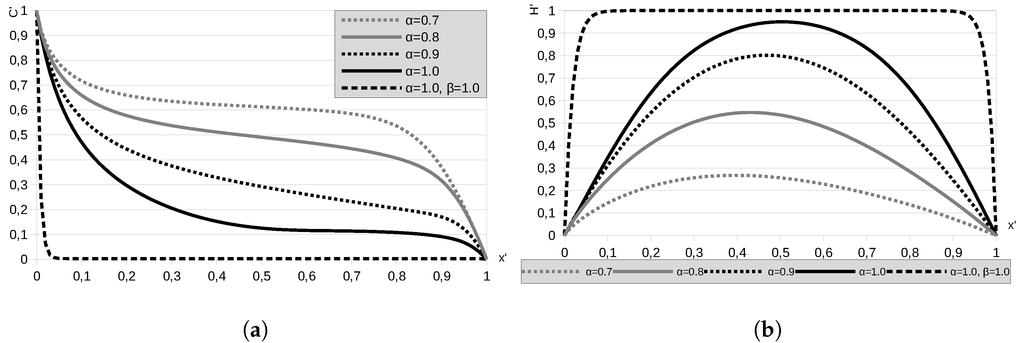
• A decrease of the fractal dimension $\alpha$ for $0<\alpha <1$ results in both an acceleration of salinization processes in the compacting massif (Figure 2a), and an acceleration of water head dispersion in it (Figure 2b), that is, to a reduction of the compaction time compared to the case when the process is described by the fractional-differential model that takes only memory effects into account [24].
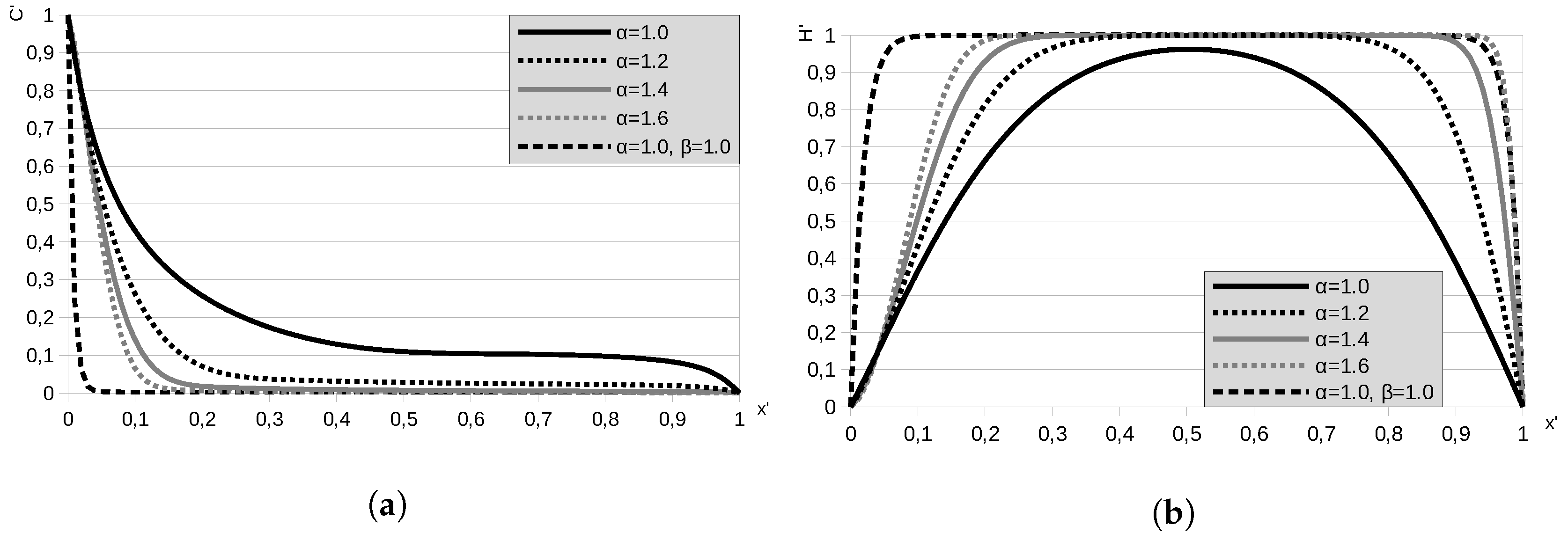
• With an increase of the fractal dimension $\alpha$ for $\alpha >1$, the processes of salinization (Figure 3a) and water heads dispersion (Figure 3b) significantly slow down compared to the case when these processes are modeled using the fractional-differential mathematical model [9,24], which indicates the presence of sub-diffusion properties in the presented fractional-fractal consolidation model.

Let us note that the above-described results are in good agreement with the results of numerical modeling on the base of the fractal advection-dispersion equation that were obtained in Reference [13] and show that the fractal formulation of the advection-dispersion equation describes both super-diffusion and sub-diffusion processes. This conclusion also holds in the case of the considered fractional-fractal mathematical model of filtration consolidation in porous media saturated with salt solutions.

5. Fractional-Fractal Model of Filtration-Consolidation Process in Clay Soils Saturated with Salt Solutions: An Exact Solution of the Boundary-Value Problem

This section presents an exact analytical solution of a specific problem of anomalous consolidation dynamics posed within the framework of the fractional-fractal approach taking into account temporal non-locality of the process of excess pressures dissipation in a soil of fractal structure. The solution is obtained for a mathematical model of consolidation dynamics of a saline-saturated porous medium, specifically for a clay soil under the conditions of temporal non-locality of the process taking into account fractal properties of a medium.

In the case of a non-local in time isothermal filtration-consolidation process in a soil of fractal structure saturated with a salt solution, taking into account the phenomena of chemical osmosis and ultrafiltration, we use the constitutive equation for diffusion flow in the form of the following Fick’s law’s generalization obtained combining fractal-fractional generalization presented in Reference [14], an approach for chemical osmosis description from Reference [16] and ultrafiltration description from Reference [17]:

$$q_C=D_t^{1-\beta }\left(-d_{*}\frac{\partial C}{\partial x^{\alpha }}+C{J}_t^{1-\beta }{u}_x+\gamma d_u\frac{\partial H}{\partial x^{\alpha }}\right),$$

(17)

where $d_u$ is the ultrafiltration coefficient, H is the water head, C is the concentration. Then, from the corresponding generalized equation of salts balance in the liquid phase, taking Equation (17) into account, we have an equation for the determination of salts concentration in the form

$$\sigma D_t^{\left(\beta \right)}C=\frac{\partial }{\partial x^{\alpha }}\left(d_{*}\frac{\partial C}{\partial x^{\alpha }}+C\frac{\partial }{\partial x^{\alpha }}\left(kH-\nu C\right)-\gamma d_u\frac{\partial H}{\partial x^{\alpha }}\right)$$

(18)

where $D_t^{\left(\beta \right)}$ is the operator of Caputo-Gerasimov fractional differentiation [19,20,21] of the order $\beta$, $0<\beta \le 1$, $\frac{\partial }{\partial x^{\alpha }}$ is the fractal derivative operator [13,15], $\alpha >0$ is the fractal dimension.

Equations (4) and (18) are the governing equations of the new fractional-fractal model that describes the dynamics of a filtration-consolidation process in saline saturated soils in the conditions of temporal non-locality taking into account their fractal properties, chemical osmosis, and ultrafiltration.

For the case of a clay soil with small filtration velocities, we follow Reference [17] and neglect the corresponding second term in the right-hand side of Equation (18). As a result, we obtain a system of equations in the form

$$D_t^{\left(\beta \right)}H=\frac{\partial }{\partial x^{\alpha }}\left(\frac{\partial }{\partial x^{\alpha }}\left(C_{\upsilon }H-\mu C\right)\right),$$

(19)

$$\sigma D_t^{\left(\beta \right)}C=\frac{\partial }{\partial x^{\alpha }}\left(\frac{\partial }{\partial x^{\alpha }}\left(d_{*}C-\gamma d_{u}H\right)\right).$$

(20)

Here, when $\alpha =1$ we have the system of equations of consolidation theory without taking into account medium’s fractal properties, but considering temporal non-locality of the process [9,10,24]. When $\alpha ,\beta =1$ we obtain the system of consolidation equations for clay soil massif in the classical formulation [17].

Within the framework of the mathematical model defined by Equations (19) and (20), the problem of modeling the dynamics of an anomalous filtration-consolidation process in the domain of finite thickness l with permeable upper boundary $x=1$ and impermeable lower boundary $x=l$ ($l>1$) is reduced to the solution for $0<t<+\infty$ of the equations’ system (19) and (20) with the following conditions:

$$H(1,t)=0,\frac{\partial H}{\partial x}(l,t)=0,H(x,0)=H_0,$$

(21)

$$C(1,t)=C_0,\frac{\partial C}{\partial x}(l,t)=0,C(x,0)=0,$$

(22)

where $H_0$ is the initial value of water head, $C_0$ is the value of salts concentration at the inlet of the filtration flow.

Below we describe a technique for obtaining a closed-form solution of the boundary value problem (19)–(22).

According to the d’Alembert’s method [28], multiplying Equation (19) by an undefined real coefficient q and adding the result to Equation (20) we obtain

$$D_t^{\left(\alpha \right)}(qH+\sigma C)=\frac{\partial }{\partial x^{\alpha }}\left(\frac{\partial }{\partial x^{\alpha }}\left(\left(q{C}_{\upsilon }-\gamma d_u\right)H+\left(d_{*}-\mu q\right)C\right)\right).$$

(23)

Further, in Equation (23) we set

$$q{C}_{\upsilon }-\gamma d_u=qr,d_{*}-\mu q=\sigma r,$$

(24)

where r is the real constant determined as follows.

From Equation (24) we have the following quadratic equation to determine r:

$$\sigma r^2-(d_{*}+\sigma C_{\upsilon })r+C_{\upsilon }{d}_{*}-\mu \gamma d_u=0.$$

(25)

From it we obtain

$$r_{1,2}=\frac{1}{2\sigma }(d_{*}+\sigma C_{\upsilon }\pm \sqrt{\Delta }),\Delta ={(d_{*}-\sigma C_{\upsilon })}^2+4\sigma \mu \gamma d_u>0.$$

(26)

The following two values of q correspond to the roots $r=r_i(i=1,2)$ of Equation (25) determined according to (26):

$$q_i=\frac{d_{*}-\sigma r_i}{\mu }(i=1,2).$$

Let

$${\psi }_i(x,t)=q_{i}H(x,t)+\sigma C(x,t)(i=1,2).$$

(27)

Taking into account (23), (24), (27), for finding unknown functions ${\psi }_i(i=1,2)$ we obtain the set of equations

$$D_t^{\left(\beta \right)}{\psi }_i=r_i\frac{\partial }{\partial x^{\alpha }}\left(\frac{\partial }{\partial x^{\alpha }}{\psi }_i(x,t)\right)(i=1,2).$$

(28)

Considering the boundary conditions (21) and (22), we have the corresponding boundary conditions for the functions ${\psi }_i(i=1,2)$ in the form

$${\psi }_i(1,t)=\sigma C_0,{\psi }_{i_x}^{{}^{\prime }}(l,t)=0,{\psi }_i(x,0)=q_i{H}_0(i=1,2).$$

(29)

Let us note that for physical correctness of the considered problems, the conditions $r_i>0(i=1,2)$ must be satisfied. Making in the problems (28) and (29) a transition to homogeneous boundary conditions using the substitutions

$$U_i(x,t)={\psi }_i(x,t)-\sigma C_0(i=1,2)$$

we obtain the following homogeneous boundary value problems for the determination of the functions $U_i(x,t)(i=1,2)$:

$$D_t^{\left(\beta \right)}{U}_i(x,t)=r_i\frac{\partial }{\partial x^{\alpha }}\left(\frac{\partial }{\partial x^{\alpha }}{U}_i(x,t)\right)(i=1,2),$$

(30)

$$U_i(1,t)=0,U_{i_x}^{{}^{\prime }}(l,t)=0,U_i(x,0)=f_i(i=1,2)$$

(31)

where $f_i=q_i{H}_0-\sigma C_0$ and $r_i(i=1,2)$ are defined by (26).

Let us introduce a finite integral transform with respect to the geometric variable x in the form [29]

$${\overline{U}}_i^{\left(n\right)}\left(t\right)={\int }_1^l{U}_i(x,t){\phi }_n^{\left(\alpha \right)}\left(x\right)\frac{dx}{x^{1-\alpha }},$$

(32)

where the eigenfunctions of the Sturm-Liouville problem and the corresponding eigenvalues are as follows:

$${\phi }_n^{\left(\alpha \right)}\left(x\right)=sin\left[{\lambda }_n^{\left(\alpha \right)}(x^{\alpha }-1)\right],{\lambda }_n^{\left(\alpha \right)}=\frac{\pi (2n-1)}{2(l^{\alpha }-1)}(n\in N).$$

(33)

Applying the transform (32) and (33) to the problems (30) and (31), taking into account the properties of the corresponding spectral boundary value problem [29]

$$x^{2a}\frac{d^2\phi }{d{x}^2}+a{x}^{2a-1}\frac{d\phi }{dx}+{\lambda }^2\phi \left(x\right)=0,\phi \left(1\right)=0,{\phi }^{\prime }\left(l\right)=0,a=1-\alpha ,$$

we obtain

$$D_t^{\left(\beta \right)}{\overline{U}}_i^{\left(n\right)}\left(t\right)+r_i{\left({\lambda }_n^{\left(\alpha \right)}\right)}^2{\overline{U}}_i^{\left(n\right)}\left(t\right)=0(i=1,2;n\in N),$$

(34)

$${\overline{U}}_i^{\left(n\right)}\left(0\right)={\theta }_i^{\left(n\right)}(i=1,2;n\in N),$$

(35)

where ${\theta }_i^{\left(n\right)}=\left(q_i{H}_0-\sigma C_0\right){\int }_1^l{\phi }_n^{\left(\alpha \right)}\left(x\right)\frac{dx}{x^{1-\alpha }}$$(i=1,2;n\in N)$.

Solutions of the problems (34) and (35) can be easily obtained by the Laplace transform method [19,20,21] and have the form

$${\overline{U}}_i^{\left(n\right)}\left(t\right)={\theta }_i^{\left(n\right)}{E}_{\beta }(-r_i{\left({\lambda }_n^{\left(\alpha \right)}\right)}^2{t}^{\beta })(i=1,2;n\in N),$$

(36)

where $E_{\beta }\left(z\right)$ is the Mittag-Leffler function [27].

As the formula for the inversion of the used finite integral transform has the form [29]

$$U_i(x,t)=\frac{2\alpha }{l^{\alpha }-1}\sum _{n=1}^{\infty }{\overline{U}}_i^n\left(t\right){\phi }_n^{\left(\alpha \right)}\left(x\right)(i=1,2),$$

returning in (36) to the domain of originals with respect to the geometric variable we obtain

$$U_i^{}(x,t)=\frac{2\alpha }{l^{\alpha }-1}\sum _{n=1}^{\infty }{\theta }_i^{\left(n\right)}{E}_{\beta }(-r_i{\left({\lambda }_n^{\left(\alpha \right)}\right)}^2{t}^{\beta }){\phi }_n^{\left(\alpha \right)}\left(x\right)(i=1,2),$$

(37)

where ${\phi }_n^{\left(\alpha \right)}\left(x\right)$ are defined by (33).

Transition to the water head and concentration functions is carried out according to the following formulas:

$$H=\frac{{\psi }_1-{\psi }_2}{q_1-q_2},C=\frac{q_1{\psi }_2-q_2{\psi }_1}{\sigma (q_1-q_2)},$$

$${\psi }_i(x,t)=U_i(x,t)+\sigma C_0(i=1,2),$$

where $U_i(x,t)(i=1,2)$ are defined by (37).

From the above-described relations, as a special case when $\alpha \to 1$, we obtain the solution of the corresponding consolidation problem in the fractional-differential formulation [9,10] without taking into account fractal properties of a medium. When $\alpha ,\beta \to 1$, the found solution directly implies the solution of the classical consolidation problem [17].

6. Conclusions

This paper is devoted to the mathematical modeling of anomalous filtration-consolidation processes in fractal-structured soils saturated with salt solutions. For a theoretical description of the peculiarities of these media’s dynamics, we proposed to use models built within the framework of the fractional-fractal approach [13,14,15]. This makes it possible to take into account temporal non-locality of the considered consolidation processes in soil massifs of fractal structure. In particular, we considered the problem of modeling the dynamics of a non-local in time filtration-consolidation process in a salt-saturated fractal medium in the case of the domain of finite thickness with permeable boundaries presenting a technique for the numerical solution of the corresponding one-dimensional boundary value problem.

We have also constructed the fractional-fractal model of a filtration-consolidation process in a clay soil massif of fractal structure saturated with a salt solution. For this model, a closed-form solution of the corresponding one-dimensional boundary value problem for the domain of finite thickness with permeable upper and impermeable lower boundaries is obtained.

References

- Bulavatsky, V.M.; Kryvonos, I.G.; Skopetsky, V.V. Non-Classical Mathematical Models of Heat and Mass Transfer Processes; Naukova Dumka: Kyiv, Ukraine, 2005. (In Ukrainian) [Google Scholar]
- Vlasiuk, A.P.; Martyniuk, P.M. Mathematical Modeling of Consolidation in Soils in the Conditions of Salt Solution Filtration; Publishing House of UDUVHP: Rivne, Ukraine, 2004. (In Ukrainian) [Google Scholar]
- Lyashko, S.I.; Klyushin, D.A.; Timoshenko, A.A.; Lyashko, N.I.; Bondar, E.S. Optimal control of intensity of water point sources in unsaturated porous medium. J. Autom. Inf. Sci. 2019, 51, 24–33. [Google Scholar] [CrossRef]
- Bomba, A.Y.; Hladka, O.M. Methods of Complex Analysis of Parameters Identification of Quasiideal Processes in Nonlinear Doubly-layered Porous Pools. J. Autom. Inf. Sci. 2014, 46, 50–62. [Google Scholar] [CrossRef]
- Florin, V.A. Fundamentals of Soil Mechanics; National Technical Information Service: Moscow, Russia, 1961.
- Zaretsky, I.K. Theory of Soil Consolidation; Nauka: Moscow, Russia, 1967. (In Russian) [Google Scholar]
- Shirinkulov, T.S.; Zaretsky, I.K. Creep and Consolidation of Soils; Fan: Tashkent, Uzbekistan, 1986. (In Russian) [Google Scholar]
- Ivanov, P.L. Soils and the Bases of Hydro-Technical Facilities; Vysshaja Shkola: Moscow, Russia, 1991. (In Russian) [Google Scholar]
- Bulavatsky, V.M.; Kryvonos, Y.G. The numerically analytical solutions of some geomigratory problems within the framework of fractional-differential mathematical models. J. Autom. Inf. Sci. 2014, 46, 1–11. [Google Scholar] [CrossRef]
- Bulavatsky, V.M. Fractional differential mathematical models of the dynamics of nonequilibrium geomigration processes and problems with nonlocal boundary conditions. Cybern. Syst. Anal. 2014, 50, 81–89. [Google Scholar] [CrossRef]
- Bulavatsky, V.M. Some modelling problems of fractional-differential geofiltrational dynamics within the framework of generalized mathematical models. J. Autom. Inf. Sci. 2016, 48, 27–41. [Google Scholar] [CrossRef]
- Bulavatsky, V.M.; Bohaienko, V.O. Numerical simulation of fractional-differential filtration-consolidation dynamics within the framework of models with non-singular kernel. Cybern. Syst. Anal. 2018, 54, 193–204. [Google Scholar] [CrossRef]
- Allwright, A.; Atangana, A. Fractal advection-dispersion equation for groundwater transport in fractured aquifers with self-similarities. Eur. Phys. J. Plus 2018, 133, 1–14. [Google Scholar] [CrossRef] [Green Version]
- Chen, W. Time-space fabric underlying anomalous diffusion. Chaos Soliton. Fract. 2006, 28, 923–929. [Google Scholar] [CrossRef] [Green Version]
- Cai, W.; Chen, W.; Wang, F. Three-dimensional Hausdorff derivative diffusion model for isotropic/anisotropic fractal porous media. Therm. Sci. 2018, 22, S1–S6. [Google Scholar] [CrossRef]
- Kooi, H.; Garavito, A.M.; Bader, S. Numerical modelling of chemical osmosis and ultrafiltration across clay formations. J. Geochem. Explor. 2003, 78, 333–336. [Google Scholar] [CrossRef]
- Kaczmarek, M.; Huekel, T. Chemo-mechanical consolidation of clays: Analytical solution for a linearized one-dimensional problem. Transp. Porous Media 1998, 32, 49–74. [Google Scholar] [CrossRef]
- Liashko, I.I.; Demchenko, L.I.; Mystetsky, H.E. Numerical Solution of the Problems of Heat and Mass Transfer in Porous Media; Naukova Dumka: Kyiv, Ukraine, 1991. (In Russian) [Google Scholar]
- Podlubny, I. Fractional Differential Equations; Academic Press: New York, NY, USA, 1999. [Google Scholar]
- Kilbas, A.A.; Srivastava, H.M.; Trujillo, J.J. Theory and Applications of Fractional Differential Equations; Elsevier: Amsterdam, The Netherlands, 2006. [Google Scholar]
- Sandev, T.; Tomovsky, Z. Fractional Equations and Models. Theory and Applications; Springer: Cham, Switzerland, 2019. [Google Scholar]
- Samko, S.G.; Kilbas, A.A.; Marichev, O.I. Fractional Integrals and Derivatives: Theory and Applications; Gordon and Breach: New York, NY, USA, 1993. [Google Scholar]
- Eidelman, S.D.; Kochubei, A.N. Cauchy problem for fractional diffusion equations. J. Differ. Equ. 2004, 199, 211–255. [Google Scholar] [CrossRef] [Green Version]
- Bulavatsky, V.M. Mathematical Model of Geoinformatics for Investigation of Dynamics for Locally Nonequlibrium Geofiltration Processes. J. Autom. Inf. Sci. 2011, 43, 12–20. [Google Scholar] [CrossRef]
- Samarskii, A. The Theory of Difference Schemes; CRC Press: New York, NY, USA, 2001. [Google Scholar]
- Abramovitz, M.; Stegun, I.A. Handbook of Mathematical Functions; Dover: New York, NY, USA, 1965. [Google Scholar]
- Gorenflo, R.; Kilbas, A.A.; Mainardi, F.; Rogosin, S.V. Mittag-Leffler Functions, Related Topics and Applications; Springer: Berlin, Germany, 2014. [Google Scholar]
- Matveev, N.M. Methods of Ordinary Differential Equations Integration; Vysheishaia Shkola: Minsk, Belarus, 1974. (In Russian) [Google Scholar]
- Martynenko, N.A.; Pustylnikov, L.M. Finite Integral Transformations and Their Application to the Analysis of Distributed Parameters Systems; Nauka: Moscow, Russia, 1986. (In Russian) [Google Scholar]
Figure 1.
Dimensionless concentration (a) and water head where P is the pore pressure (b) depending on dimensionless space variable in the dimensionless moments of time for , g/L, m, m, days.
Figure 2.
Dimensionless concentration (a) and water head where P is the pore pressure (b) depending on dimensionless space variable in the dimensionless moments of time for , , g/L, m, m, days.
Figure 3.
Publisher’s Note: MDPI stays neutral with regard to jurisdictional claims in published maps and institutional affiliations. |
© 2020 by the authors. Licensee MDPI, Basel, Switzerland. This article is an open access article distributed under the terms and conditions of the Creative Commons Attribution (CC BY) license (http://creativecommons.org/licenses/by/4.0/).
Share and Cite
MDPI and ACS Style
Bohaienko, V.; Bulavatsky, V. Fractional-Fractal Modeling of Filtration-Consolidation Processes in Saline Saturated Soils. Fractal Fract. 2020, 4, 59. https://0-doi-org.brum.beds.ac.uk/10.3390/fractalfract4040059
AMA Style
Bohaienko V, Bulavatsky V. Fractional-Fractal Modeling of Filtration-Consolidation Processes in Saline Saturated Soils. Fractal and Fractional. 2020; 4(4):59. https://0-doi-org.brum.beds.ac.uk/10.3390/fractalfract4040059
Chicago/Turabian StyleBohaienko, Vsevolod, and Volodymyr Bulavatsky. 2020. "Fractional-Fractal Modeling of Filtration-Consolidation Processes in Saline Saturated Soils" Fractal and Fractional 4, no. 4: 59. https://0-doi-org.brum.beds.ac.uk/10.3390/fractalfract4040059