Article

Application of Fractal Dimension of Terrestrial Laser Point Cloud in Classification of Independent Trees

1
School of Remote Sensing and Information Engineering, Wuhan University, Wuhan 430072, China
2
Chang Guang Satellite Technology Co., Ltd., Changchun 251500, China
3
School of Resource and Environmental Sciences, Wuhan University, Wuhan 430072, China
*
Author to whom correspondence should be addressed.
Submission received: 27 November 2020 / Revised: 19 January 2021 / Accepted: 27 January 2021 / Published: 1 February 2021

Abstract

:
Tree precise classification and identification of forest species is a core issue of forestry resource monitoring and ecological effect assessment. In this paper, an independent tree species classification method based on fractal features of terrestrial laser point cloud is proposed. Firstly, the terrestrial laser point cloud data of an independent tree is preprocessed to obtain terrestrial point clouds of independent tree canopy. Secondly, the multi-scale box-counting dimension calculation algorithm of independent tree canopy dense terrestrial laser point cloud is proposed. Furthermore, a robust box-counting algorithm is proposed to improve the stability and accuracy of fractal dimension expression of independent tree point cloud, which implementing gross error elimination based on Random Sample Consensus. Finally, the fractal dimension of a dense terrestrial laser point cloud of independent trees is used to classify different types of independent tree species. Experiments on nine independent trees of three types show that the fractal dimension can be stabilized under large density variations, proving that the fractal features of terrestrial laser point cloud can stably express tree species characteristics, and can be used for accurate classification and recognition of forest species.

1. Introduction

Plants play an important role in the whole ecosystem because of their important impact on the ecological environment [1,2,3]. Tree species classification is the first basic work for correct understanding and research of trees [4,5,6]. It is also the core issue of remote sensing monitoring of forestry resources and ecological effect assessment [7,8]. Urban ecological construction and greening are important aspects of urban development [9]. This process not only considers the number of trees planted, but also fully considers the allocation of plant species to optimize urban environment from biomass and carbon balance [10,11,12]. At the same time, in the construction of smart cities and smart gardens, tree species classification is also important for automatic tree modeling [13].
Research on the identification and classification of tree species has focused on the appearance characteristics of plants, especially in the early period, mainly using 2D images of trees to identify tree species by extracting the shape of tree leaves. Guyer et al. [14] extracted 17 features to describe leaf shape in 1993 to classify plants. Abbasi et al. [15,16] used multi-scale curvature space to describe the boundaries and shapes of leaves and other features to classify chrysanthemums. Fu et al. [17] carried out a preliminary study on automatic plant classification in 1994. Qi et al. [18] established a plant classification recognition model to study plant classification by extracting leaf size, leaf shape, circularity parameters and leaf margins. In 2003, Wang et al. [19] proposed a new shape description method, CCD (centroid-countour distance), which can describe shape more effectively from a global perspective. However, because some plants and their varieties have similar leaf shapes, it is limited and difficult to use computer graphics and image recognition methods to classify and recognize plants simply according to their leaves.
In the past decade, Light Detection and Ranging technology has been widely used in the field of agricultural and forestry vegetation remote sensing [20,21,22,23] due to its high-precision and high-density 3D spatial information acquisition capability. High density terrestrial laser point clouds data can obtain accurate horizontal and vertical vegetation distribution structure [24,25,26,27]. It can provide not only stand-scale vegetation parameters, but also individual-tree-scale vegetation parameters. It plays an important role in vegetation survey, identification of complex tree species, inversion of vegetation parameters such as leaf area index (LAI) and chlorophyll content in canopy, analysis of forest stock, biomass and carbon sequestration potential [28,29]. It is an appropriate method to use fractal theory to analyze, process and classify the laser point cloud structure of independent tree, because of the remarkable scattering and non-linearity.
The research results of fractal theory and fractal technology in remote sensing field show that, fractal is very suitable for object expression with nonlinear and self-similar characteristics [30,31,32]. In fact, fractal dimension has been widely used to generate expressions of different types of trees in the field of forest visual computing, forest tree species simulation and forest modeling expression. L-system (Lindenmayer system) is an algorithm proposed by Aristid Lindenmayer in 1968 [33,34]. It can describe processes such as the growth of plants. References [35,36] used L-system to simulate the basic shape of trees, stochastic L-system to simulate the growth of apical buds, and control the growth direction of branches to simulate the phototaxis and geotaxis of tree growth. Iterated function system (IFS) theory, introduced by Zadeh [37], is an extension of fuzzy set theory and more suitable for explaining human thinking than fuzzy set theory. IFS theory is a powerful way to deal with uncertainty and vagueness, and was introduced by Atanassov [38]. Zhong et al. [39] constructed tree mathematical model, proposed a three-dimensional tree simulation method, and constructed a visualization system based on IFS theory [40]. Wang Xiaoming [41] put forward tree simulation methods based on skeleton customization and particle system model, the branch and leaf model was generated by particle system method, and the branch growth model was achieved based on these static models.
It can be seen that fractal dimension values are widely used in ecology, but independent tree species classification based on fractal characteristics of terrestrial laser point clouds is less studied. Zheng et al. [42] used terrestrial laser point cloud data to calculate the fractal dimension of tree canopy, but only sparse point cloud data was used, and there was no validation of whether the fractal value remained stable during the decline of point cloud data. In this study, by using the dense terrestrial laser point cloud data of different types of independent tree species, the fractal algorithm is used to calculate the fractal dimension of terrestrial point clouds data and achieve the classification of independent tree species according to the fractal characteristics of natural tree canopy.

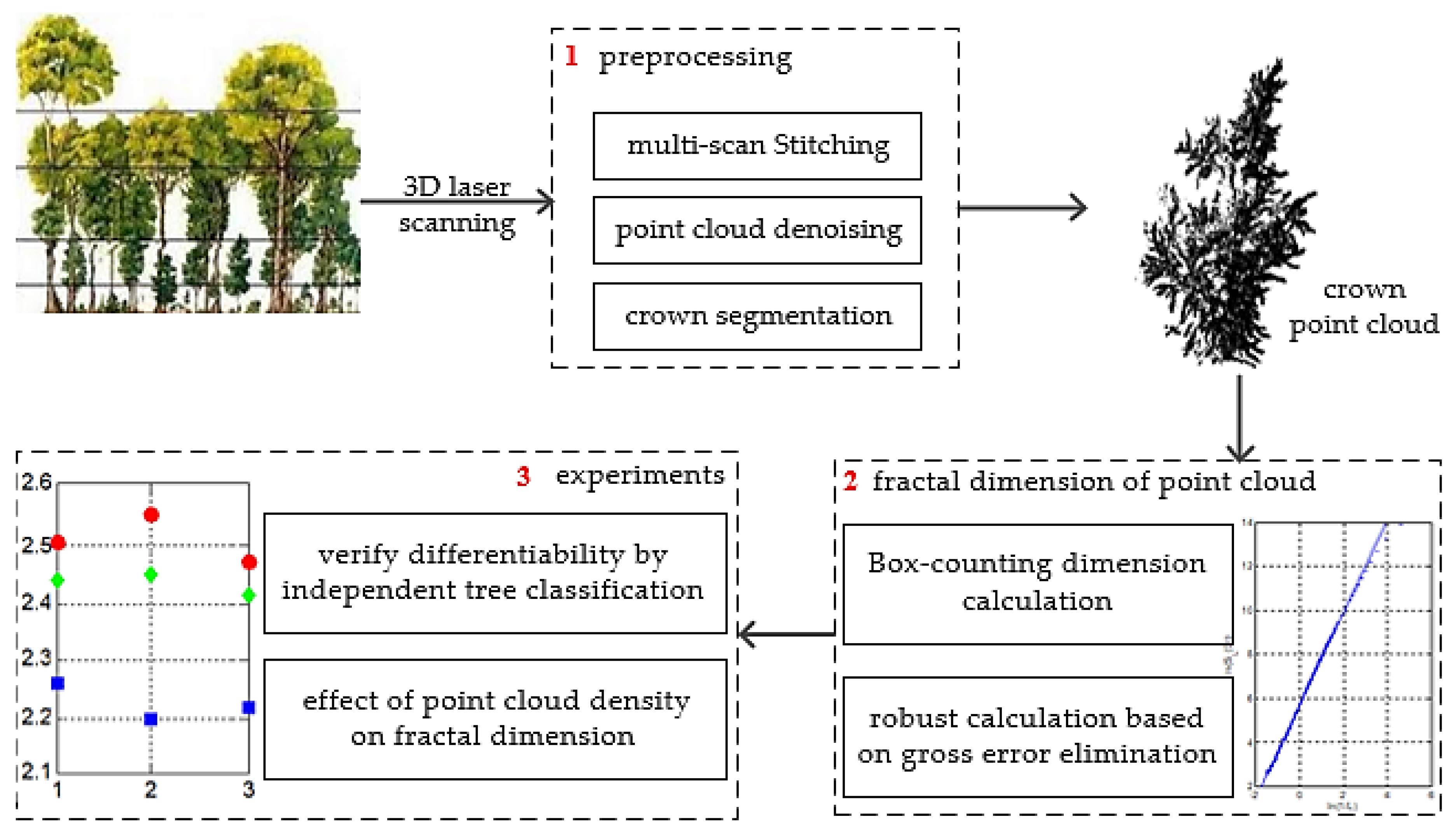
2. Materials and Methods

The ractal analysis method was introduced to tree species classification using terrestrial laser point clouds in this study. Point clouds of trees were obtained by using terrestrial laser scanner, and fractal dimension values of point clouds of different tree species were calculated. The classification of tree species could be achieved according to the fractal dimension features. The whole technical process is shown in Figure 1.

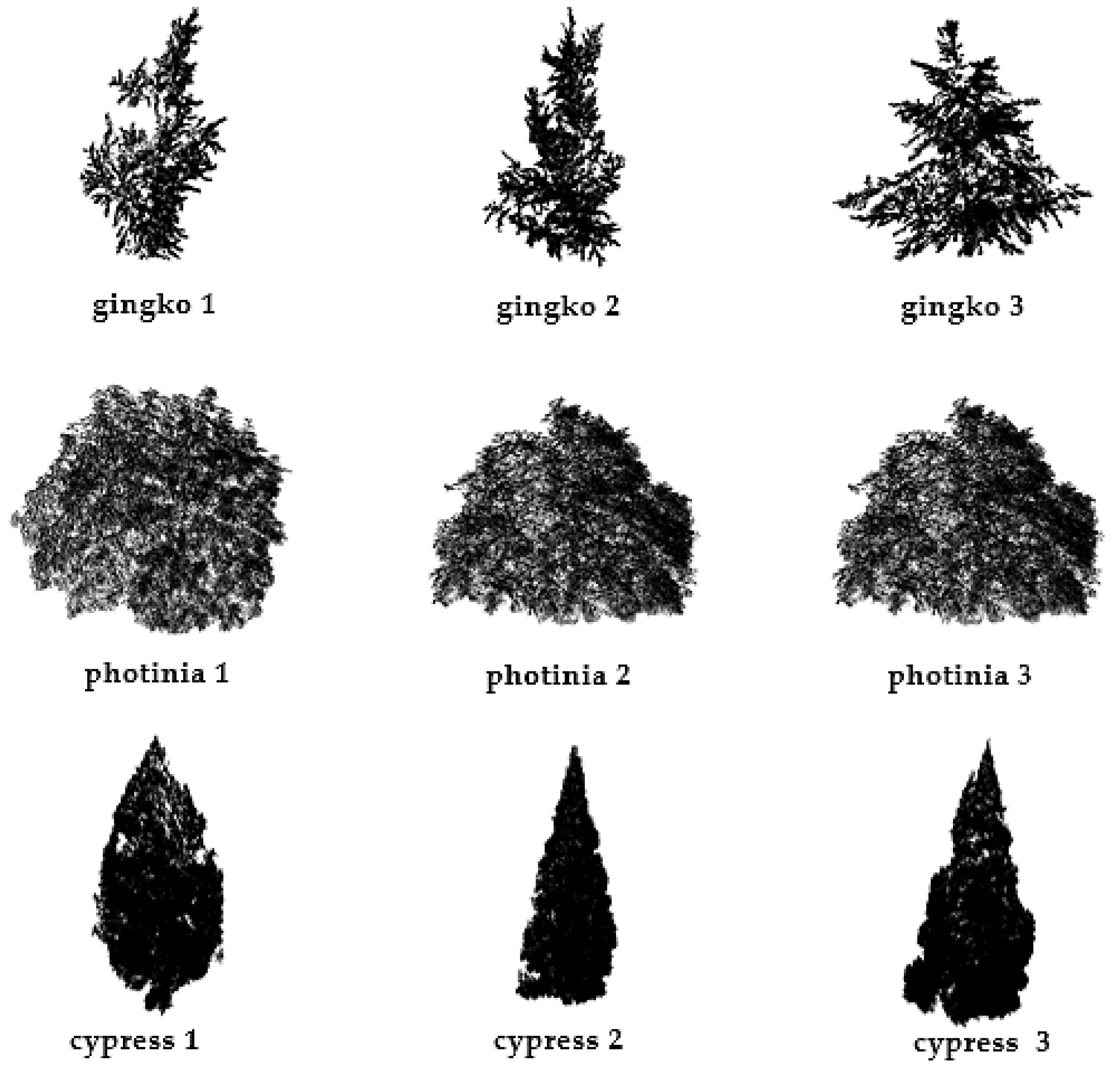
2.1. Independent Tree Point Cloud Acquisition and Preprocessing

3D terrestrial laser scanner (TLS) is an efficient method to acquire accurate field data and measure parameters of low-stature vegetation, such as coverage, leaf area index (LAI), and tree height, because it has strong penetration and is not influenced by the light, location and weather [43,44,45]. We scanned the trees using the RIEGL VZ-400i TLS (Horn, Austria) mounted on a tripod. The VZ-400i TLS has a field view of 360° horizontal (H) × 100° vertical (V), a laser pulse repetition rate of up to 1.2 MHz, and an accuracy of ±5 mm at a range up to 400 m, with a customizable scan spacing. This TLS unit acquires terrestrial laser point clouds at a speed up to 500,000 points per second. In this paper, a RIEGL VZ-400i TLS was used to obtain point clouds of three Gingko trees with leaves, three Photinia trees and three Cypress trees, as shown in Figure 2.
The measurement range, scanning angle and laser beam’s penetration ability of the laser scanner are limited, so obtaining complete 3D spatial information of objects at one scan is not feasible. In order to obtain more complete 3D spatial information, it is necessary to select a suitable and visible angle around trees to conduct multi-station scanning. Multiple scanning stations help reduce the occlusion caused by rugged terrain and improve the density of point clouds [46]. Prior to the scan, 4 surveyor’s poles were uniformly placed along contour line of valley slope to help conduct point cloud registration. After rough registration, multi-station point clouds would be spliced optimally by using Iterative Closest Point (ICP) algorithm [47]. Spliced point cloud data would be clipped according to the range of the tree, and only point clouds of the canopy would be reserved, while point clouds of unrelated objects would be removed. During the multi-station scanning process, the overlapping area of the tree would generate repeated points because of multiple scans. Therefore, duplicate points that are in the individual tree point cloud need to be removed, and the final terrestrial point clouds of an individual tree could be obtained.

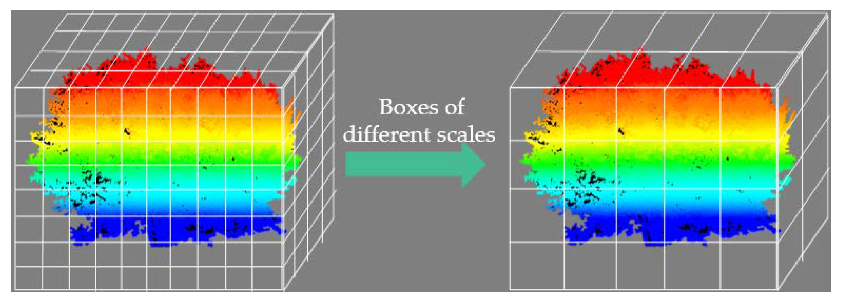
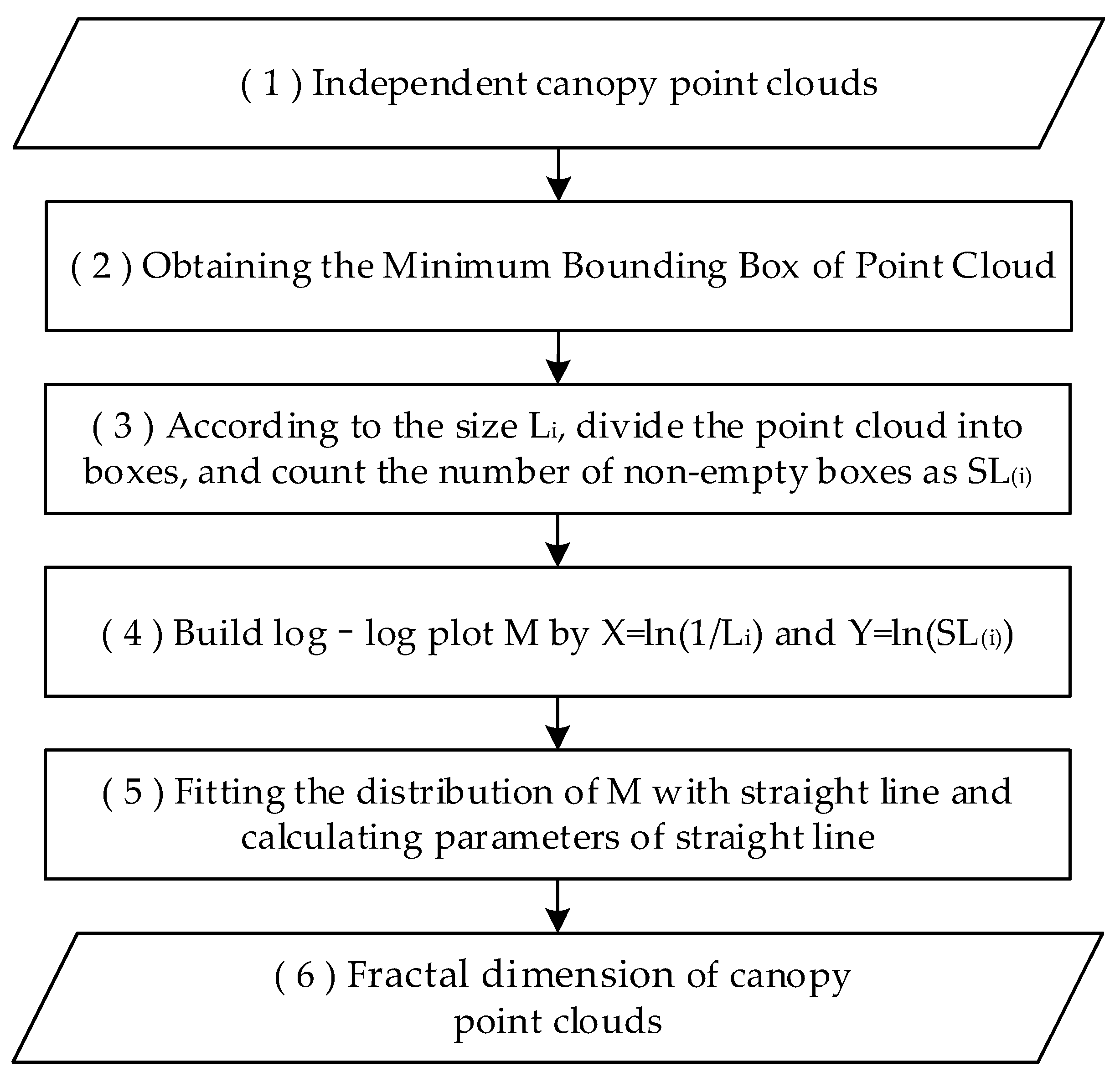
2.2. Box-Counting of Terrestrial Point Clouds

The box-counting dimension is the most widely-used fractal dimension calculation method [48,49,50,51]. The box-counting dimension is one of the most popular fractal dimensions, which is applicable to simple fractals as well as complex fractals. The essence of box-counting dimension is to change the degree of coarse visualization to measure the figure, usually starting from counting large boxes, and then decreasing the scale of boxes, only counting those “non-empty” boxes [52]. Let n in N , F be a non-empty bounded subset in R n , and N L ( F ) be the smallest number of cubes (in R n ) of side L that cover F [53]. The box-counting dimension of F was defined by Equation (1):
d i m B F = l i m L 0 l o g N L ( F ) l o g L
In this study, considering the characteristics of terrestrial laser point cloud data of individual trees, we use multi-scale cube coverage that based on the range of an individual tree, to calculate the fractal dimension of an individual tree. The schematic diagram is shown in Figure 3.
In Equation (1), reference [53] indicated that if the limit exists, to calculate the limit when L 0 , we only have to consider the limit of any descending series L i , which satisfy L i + 1 c L i , when it approach 0, and c satisfy 0 < c < 1 , especially when δ k = c i . In this study, considering the dividing process would be performed on whole terrestrial point clouds iteratively, so the number of iterations of spatial divisions ( I t e r a t o r ) need to be determined by the shortest side length ( L m i n ) of the bounding rectangle of the terrestrial point clouds and the initial side length ( L 0 ) of the box. Using the simplest linear sequence, the number of iterations I t e r a t o r was determined by Equation (2):
I t e r a t o r = L m i n 2 × L 0
and the side length of box L i at iteration i was determined by Equation (3):
L i = L 0 × i ( i = 1 , 2 , 3 , I t e r a t o r )
After specifying the way and step of box-dividing, the main process of calculating the fractal dimension of terrestrial point clouds is shown in the Figure 4.
First of all, parameters of the bounding box of an individual tree’s point cloud need to be obtained, and these parameters can help determine the spatial range of the point cloud of an individual tree and the coordinates of the start point of the spatial box. Then, the initial side length of the box would be set. Considering that point cloud data has high accuracy and large density, the initial side length of the box cannot be set with a large value. In this paper, we set the initial side length of the box to 0.01 m. We use an integer that is not greater than the quotient of the half of the shortest side length divided by the initial side length as the number of iterations, it can effectively avoid the excessively small number of spatial dividing boxes or only one box containing all point cloud data, which were caused by excessively large number of iterations. During the process of each iteration, the space that the point cloud of an individual tree took up was first divided by spatial boxes, whose side length was L i . Then, we would determine the number of boxes that contained point clouds ( S L i ( D ) ) and recorded the reciprocal of side length ( 1 L i ). The logarithms of S L i ( D ) and 1 L i became the coordinates of a point, M i ( ln ( 1 L i ) , ln ( S L i ( D ) ) ) , in the point set of the double logarithmic scatter plots (log-log plot M ).

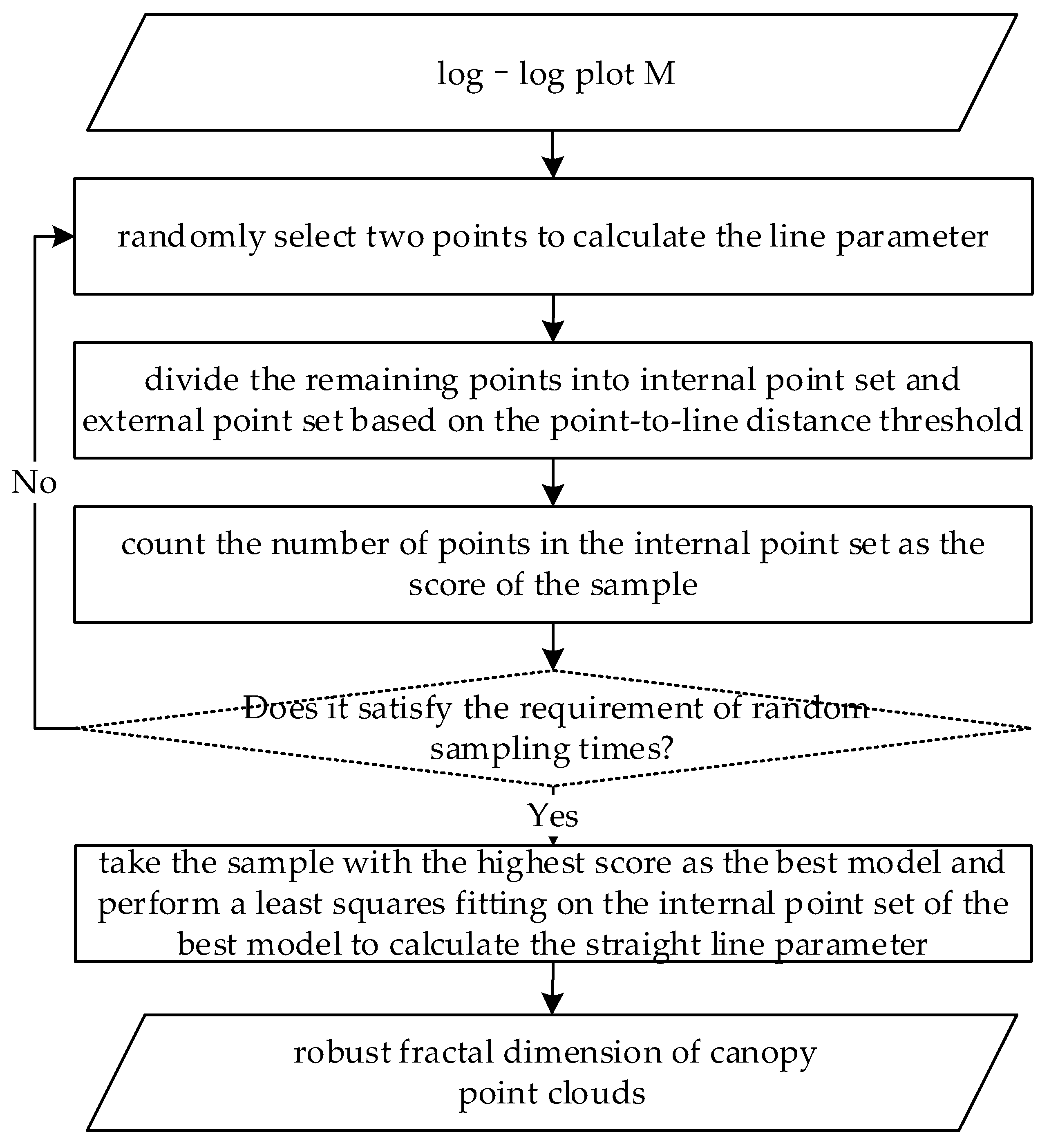
2.3. Box-Counting Dimension Fitting Based on RANSAC Gross Error Elimination

The point set of the double logarithmic scatter plots was obtained after completing dividing spatial box for I t e r a t o r times. Points in the point set were fitted with a straight line by using the least squares method, and the slope of the fitted line was the fractal dimension. Considering that the slope of the fitted straight line was the fractal dimension of an individual tree, the dimension of an individual tree could not be infinite. y = k x + b was used to obtain the equation of the fitted straight line.
Random Sample Consensus algorithm (RANSAC) was first proposed by Fischler and Bolles [54] in 1981. This algorithm calculated parameters of a mathematical model according to a set of sample data, which contained abnormal data, and thus valid sample data would be extracted from the data set while abnormal sample data would be eliminated. RANSAC could help eliminate abnormal data from the point set of the log-log plot during the straight-line fitting process, and therefore more accurate and more robust fractal dimension of the terrestrial point clouds of an individual tree would be obtained.
When the RANSAC algorithm was used to eliminate abnormal data from the point set of the log-log plot, it is necessary to fully consider the characteristics of the point set to set proper number of iterations and other parameters. Characteristics of the point set of the log-log plot were as follows:
  • Data in the point set of the log-log plot only conform to linear models;
  • There is no same point in the point set of the log-log plot. Each point in the point set corresponded to a spatial partition, and side length of the box in each partition was different (the side length would be monotonically increasing from initial side length as the iterative spatial partition proceeds). Accordingly, the abscissa of every point in the point set of the log-log plot was different, and parameters of the straight line could be fitted from any two points in the point set;
  • The spatial extent of the terrestrial point clouds of an individual tree was limited, so the number of points in the point set of the log-log plot would not be excessively large.
The RANSAC algorithm could obtain all possible linear models in the point set of the log-log plot during the iterative process, and the number of iterations could be calculated by using Equation (4):
C N u m 2 = N u m × ( N u m 1 ) 2
The flow chart of the method of calculating box-counting dimensions of point clouds based on the RANSAC gross error elimination algorithm, is shown in Figure 5.

2.4. Evaluating Indicator

The slope of the straight line, namely the box-counting dimension, and the intercept of the line could be obtained by The Least Squares Approximation. The accuracies of these two parameters would be calculated by multiplying the arithmetic square root of the diagonal elements in co-factor matrix ( ( A T A ) 1 ) of Δ by root mean square error (RMSE) with unit weight ( δ ^ o ). δ ^ o could be obtained by Equation (5). The relevant formula derivation and symbolic expression can be seen in the basic principle of Least Squares Approximation.
δ ^ o = V T V I t e r a t o r 2

3. Results

3.1. Fractal Dimension of Three Ginkgo Trees

Fractal dimensions of three Ginkgo trees with foliage were calculated by setting the initial side length of the box to 0.01 m. The log-log scatter plots were presented in Figure 6, the fitting results based general least squares method were presented in Table 1, and the results based on the RANSAC gross error elimination algorithm were presented in Table 2.
It can be seen from Table 1 that the value of fractal dimension of Ginkgo trees with foliage fluctuated around 2.09. The number of points in the point cloud of No.1 tree is the least, and the number of points in its corresponding double logarithmic points set ( M 1 ) was 309 and the precision was relatively the lowest. While the number of points in the point cloud of No.3 tree is the most, and the number of points in its corresponding double logarithmic points set ( M 3 ) was 421 and the precision was relatively the highest.
By comparing Table 1 and Table 2, it was clear that the RMSEs of the unit weight, the slope and the intercept of the straight line, which was fitted by the double logarithmic points set, were greatly improved after introducing the RANSAC algorithm to eliminate the gross error, and the accuracy and the robustness of the fractal dimension of the terrestrial point clouds of an individual tree were also improved.

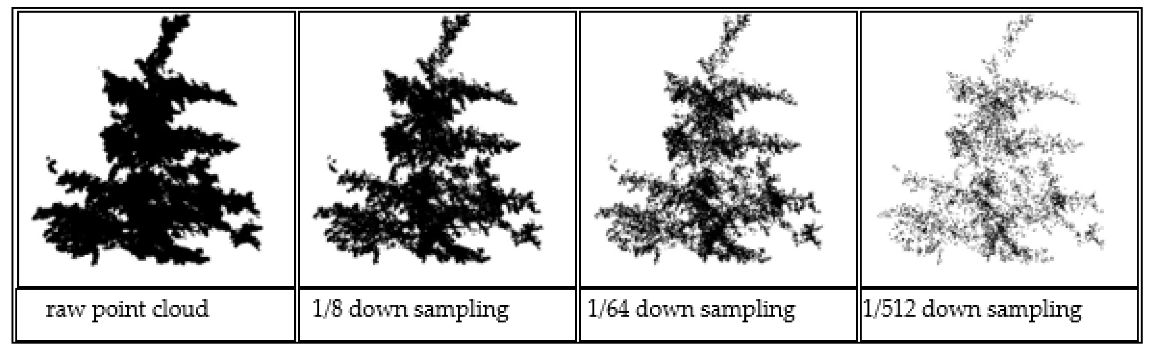
3.2. Effect of Point Cloud Density on Fractal Dimension

The results showed that point cloud density had a certain influence on the accuracies of the slope and the intercept of the fitted straight line. Because of the difference in the age, size and density of the trees, the range and density of the scanner, and the accuracy parameters, the number and density of point clouds collected from the same tree species and different tree species, even the same tree at different times are different. It is necessary to explore the influence of the number and density of the point cloud of the independent tree on the fractal dimension.
The effects of number and density of terrestrial point clouds on the fractal dimension were investigated using ginkgo and photinia trees 1 to 3. During the random down sampling process, the number of point clouds in the point cloud data is down sampled to one-half each time until the number of point clouds is less than 10,000 points. The RANSAC initial distance threshold is 0.001, and the iteration threshold step is 0.001. The data usage ratio is not less than 50% of the original double logarithmic points.

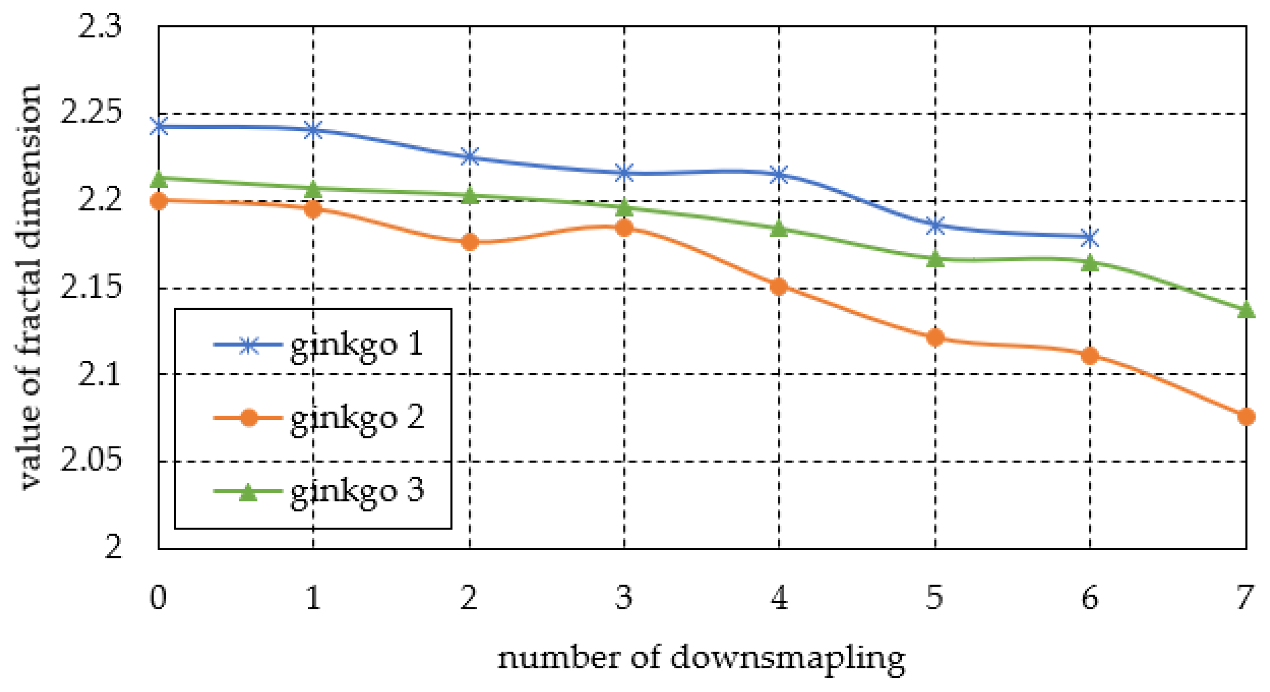
3.2.1. The Experimental Results of the Ginkgo Trees

The fractal dimension results of the ginkgo trees 1 to 3 with different number and density are shown in Table 3.
According to Table 3, it can be concluded that the fractal dimension values are decreasing as the number of point clouds decreases rapidly, and RMSE slope, intercept and unit weight are also reducing. The trend of the fractal dimension with point cloud down sampling of ginkgo trees 1 to 3 is shown in Figure 7.
Figure 7 shows that the fractal dimension values of the three ginkgo trees remain stable overall during the point cloud data down sampling process, especially when the number of point clouds is down sampled to half of the original data for the first time. Since the fact that the amount of data measured twice is doubled is rare in actual data collection, the geometric dimension method based on the RANSAC iteration threshold is robust. After down sampling of the original data fifth times, the fractal dimension values showed a relatively large decrease. We show the independent tree canopy point clouds data after the last down sampling in Figure 8. These point clouds cannot fully describe the spatial structure of the independent tree compared with the initial point cloud data of the independent tree canopy.

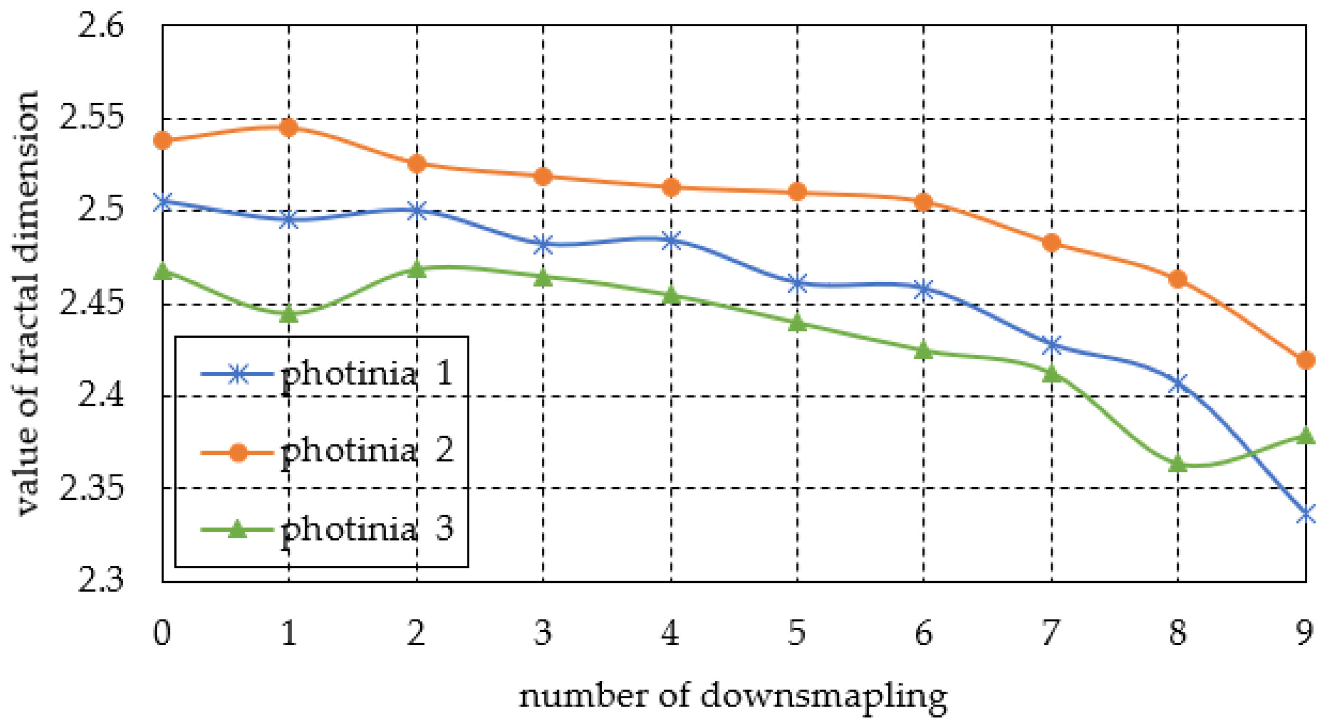
3.2.2. The Experimental Results of the Photinia Trees

The fractal dimension results of the photinia trees 1 to 3 with different number and density are shown in Table 4.
According to Table 4, it can be concluded that as the number of point clouds decreases rapidly, the fractal dimension decreases wholly, but increases slightly in very few places. At the same time, the RMSE of slope, intercept and the accuracy of unit weight are also reducing. The accuracy reduces rapidly especially in the sixths and ninth groups. The trend of the fractal dimension of the photinia trees 1 to 3 with point cloud sampling is shown in Figure 9.
The photinia tree is more complex than the ginkgo tree since its trunk begins to have multiple main branches near the ground, which makes it have a sudden change in the numerical calculation and precision of the fractal dimension. As the number of point clouds decreases, low-density point clouds are not sufficient to accurately describe the complex three-dimensional structure of the heather tree, but it can be stable in a certain range when the number of point clouds is sufficient. When the number of point clouds is too small, the number of point clouds contained in the non-empty box is too small during the space division process, so that the number of non-empty boxes is related to the number of point clouds, and the number of samples used to fit the line is also reducing, so that the fractal dimension accuracy is decreasing.
In summary, the fractal dimension of terrestrial point clouds of tree canopy is related to the number and density of the point cloud. When the laser point cloud data and density can describe the canopy structure features, the box-counting dimension method based on the RANSAC algorithm can robustly calculate the fractal dimension value of terrestrial point clouds. The number of terrestrial point clouds data in the controllable number of point clouds, and the fractal dimension values can be stable within a certain range. The fractal dimension values of different ginkgo and photinia trees are distributed in different numerical intervals, and the fractal dimension values of the same tree species are close.

4. Discussion and Conclusions

According to the fractal characteristics of the natural tree canopy, this paper proposes an independent tree species classification method based on the fractal expression of terrestrial point clouds. Firstly, dense terrestrial laser point clouds data of different types of independent trees are obtained by multi-station scanning with terrestrial laser scanner. Then, the fractal dimension values of terrestrial point clouds data are calculated by box-counting fractal method using RANSAC gross error elimination. Finally, the fractal dimension is used to classify different tree canopy morphological species. The experimental results show that the fractal dimension can describe the characteristics of different types of independent trees, and can effectively achieve the tree species classification of independent trees. It verified the feasibility and validity of the fractal theory to introduce the dense terrestrial laser point clouds feature expression. It has broad application prospects for the recognition of 3D spatial morphology of vegetation and dense terrestrial laser point clouds data intelligent processing.
Unlike the tree species classification research based on 2D image [14,15,16,19], this paper collects terrestrial point clouds data, which has richer morphological structure information compared with image data and can better reflect the structural characteristics of independent trees. This paper classifies tree species based on fractal dimensional features of tree crowns, which is simpler and ensures accuracy compared with other tree species classification methods that extract features such as tree trunk skeleton and leaf shape [55,56]. Compared with random forest, support vector machines, decision tree and other methods [55,57,58,59] that need to collect a large amount of sample data for pre-training, this paper does not have a training process, the preliminary workload is small, does not require a large amount of sample data, and costs less in labor and time. In addition, the tree species classification by using Bayes classifier or linear discriminant analysis is not effective when the number of trees is small [60,61]. From Table 1 and Table 2, it can be seen that the box-counting dimension fitting based on RANSAC gross error elimination method used in this paper has stronger robustness and is less affected by the number of trees.
The fractal characteristics of three fractal ginkgo trees, three photinia trees and three cypress trees were calculated according to the proposed method. In the calculation, the RANSAC algorithm uses the initial distance threshold of 0.001, the iteration threshold step size is set to 0.001, and the RANSAC data usage ratio is not less than 50% of the original double logarithmic points set. The results are shown in Table 5. In the table the “NofPC” means the number of points in point clouds; the “NofLP” means the number of points in the double logarithmic plot; the “DTofR” means the distance threshold setting in RANSAC; the “URofR” means the data usage ratio of RANSAC; the “FD” means the fractal dimension; and the “RMSE” means the RMSE of fractal dimension.
The distribution of fractal dimension values of each tree point cloud is shown in Figure 10. It shows that the fractal dimension values of Ginkgo, Photinia and Cypress trees are distributed in different intervals. Therefore, the fractal dimension values of independent terrestrial point clouds can be used to accurately classify the three types of trees.
Although more accurate fractal dimensions of point clouds were obtained in this study, only nine sets of point clouds of individual trees, which were from three tree species, were used in the experiment. In order to classify individual trees more meticulously, point clouds of more tree species and a larger number of individual trees need to be collected to verify the ubiquity of the proposed method. Furthermore, although data acquired from terrestrial laser scanning (TLS) system was of high quality and large density, the whole acquisition process was time-consuming, and a large range of point clouds of individual trees could not be acquired in a short time.
In fact, fractal characteristics of the terrestrial point clouds were not restricted to the overall tree canopy, and typical fractal features could also be found on a certain section of the canopy. Vertical multi-angle slicing and horizontal multi-layer slicing should be performed on point clouds of individual trees, and fractal dimensions of point cloud slices should be calculated to explore fractal features of individual trees details [62]. In addition, for trees, there are deciduous trees and evergreen trees, and for deciduous trees, point clouds collected in different seasons might be different, which might affect the calculation results of fractal dimensions.

Author Contributions

Conceptualization, J.Z. and Q.H.; Data curation, J.Z. and H.W.; Formal analysis, J.Z.; Funding acquisition, Q.H. and J.S.; Investigation, J.Z.; Methodology, J.Z.; Project administration, Q.H.; Resources, Q.H.; Software, H.W.; Supervision, J.S.; Validation, P.Z.; Visualization, H.W.; Writing—original draft, J.Z.; Writing—review and editing, P.Z. All authors have read and agreed to the published version of the manuscript.

Funding

This research was funded by the National Key R&D Program of China, grant number No: 2017YFD0600904, and the Science and Technology Planning Project of Guangdong, China (Grand No. 2017B020218001). This research was also funded by the Key Laboratory for National Geographic Census and Monitoring, National Administration of Surveying, Mapping and Geoinformation, grant number No: 2015NGCM01.

Conflicts of Interest

The authors declare no conflict of interest.

References

  1. Lesica, P.; Allendorf, F.W. Ecological genetics and the restoration of plant communities: Mix or match? Restor. Ecol. 1999, 7, 42–50. [Google Scholar] [CrossRef]
  2. Walter, J.; Jentsch, A.; Beierkuhnlein, C.; Kreyling, J. Ecological stress memory and cross stress tolerance in plants in the face of climate extremes. Environ. Exp. Bot. 2013, 94, 3–8. [Google Scholar] [CrossRef]
  3. Savage, J.A.; Clearwater, M.J.; Haines, D.F.; Klein, T.; Mencuccini, M.; Sevanto, S.; Turgeon, R.; Zhang, C. Allocation, stress tolerance and carbon transport in plants: How does phloem physiology affect plant ecology? Plant Cell Environ. 2016, 39, 709–725. [Google Scholar] [CrossRef] [PubMed]
  4. Fassnacht, F.E.; Latifi, H.; Stereńczak, K.; Modzelewska, A.; Lefsky, M.; Waser, L.T.; Straub, C.; Ghosh, A. Review of studies on tree species classification from remotely sensed data. Remote Sens. Environ. 2016, 186, 64–87. [Google Scholar] [CrossRef]
  5. Ferreira, M.P.; Wagner, F.H.; Aragão, L.E.; Shimabukuro, Y.E.; de Souza Filho, C.R. Tree species classification in tropical forests using visible to shortwave infrared WorldView-3 images and texture analysis. ISPRS J. Photogramm. Remote Sens. 2019, 149, 119–131. [Google Scholar] [CrossRef]
  6. Cardoso, D.; Särkinen, T.; Alexander, S.; Amorim, A.M.; Bittrich, V.; Celis, M.; Daly, D.C.; Fiaschi, P.; Funk, V.A.; Giacomin, L.L.; et al. Amazon plant diversity revealed by a taxonomically verified species list. Proc. Natl. Acad. Sci. USA 2017, 114, 10695–10700. [Google Scholar] [CrossRef] [Green Version]
  7. Raczko, E.; Zagajewski, B. Comparison of support vector machine, random forest and neural network classifiers for tree species classification on airborne hyperspectral APEX images. Eur. J. Remote Sens. 2017, 50, 144–154. [Google Scholar] [CrossRef] [Green Version]
  8. Ballanti, L.; Blesius, L.; Hines, E.; Kruse, B. Tree species classification using hyperspectral imagery: A comparison of two classifiers. Remote Sens. 2016, 8, 445. [Google Scholar] [CrossRef] [Green Version]
  9. Li, F.; Wang, R.; Paulussen, J.; Liu, X. Comprehensive concept planning of urban greening based on ecological principles: A case study in Beijing, China. Landsc. Urban Plan. 2005, 72, 325–336. [Google Scholar] [CrossRef]
  10. Lovell, S.T.; Taylor, J.R. Supplying urban ecosystem services through multifunctional green infrastructure in the United States. Landsc. Ecol. 2013, 28, 1447–1463. [Google Scholar] [CrossRef]
  11. Yang, J.; McBride, J.; Zhou, J.; Sun, Z. The urban forest in Beijing and its role in air pollution reduction. Urban For. Urban Green. 2005, 3, 65–78. [Google Scholar] [CrossRef]
  12. Parsa, V.A.; Salehi, E.; Yavari, A.R.; van Bodegom, P.M. Analyzing temporal changes in urban forest structure and the effect on air quality improvement. Sustain. Cities Soc. 2019, 48, 101548. [Google Scholar] [CrossRef]
  13. Wu, S.G.; Bao, F.S.; Xu, E.Y.; Wang, Y.-X.; Chang, Y.-F.; Xiang, Q.-L. A leaf recognition algorithm for plant classification using probabilistic neural network. In Proceedings of the 2007 IEEE International Symposium on Signal Processing and Information Technology, Giza, Egypt, 15–18 December 2007; pp. 11–16. [Google Scholar]
  14. Guyer, D.; Miles, G.; Gaultney, L.; Schreiber, M. Application of machine vision to shape analysis in leaf and plant identification. Trans. ASAE USA 1993. [Google Scholar]
  15. Abbasi, S.; Mokhtarian, F.; Kittler, J. Reliable classification of chrysanthemum leaves through curvature scale space. In Proceedings of the International Conference on Scale-Space Theories in Computer Vision; Springer: Berlin/Heidelberg, Germany, 1997; pp. 284–295. [Google Scholar]
  16. Mokhtarian, F.; Abbasi, S. Matching shapes with self-intersections: Application to leaf classification. IEEE Trans. Image Process. 2004, 13, 653–661. [Google Scholar] [CrossRef]
  17. Fu, X.; Lu, H.; Luo, M.; Cao, W.; Yu, X. Preliminary Study on Automatical Plant Classification by Use of Computer. Chin. J. Ecol. 1994, 2, 69–71. [Google Scholar]
  18. Qi, H.; Shou, T.; Jin, S. Computer Aided Plant Recognition Model Based on Leaf Characteristics. J. Zhejiang AF Univ. 2003, 20, 281–284. [Google Scholar]
  19. Wang, Z.; Chi, Z.; Feng, D. Shape based leaf image retrieval. IEE Proc. Vis. Image Signal Process. 2003, 150, 34–43. [Google Scholar] [CrossRef]
  20. Lefsky, M.A.; Cohen, W.B.; Parker, G.G.; Harding, D.J. Lidar remote sensing for ecosystem studies: Lidar, an emerging remote sensing technology that directly measures the three-dimensional distribution of plant canopies, can accurately estimate vegetation structural attributes and should be of particular interest to forest, landscape, and global ecologists. BioScience 2002, 52, 19–30. [Google Scholar]
  21. Chen, Q.; Qi, C. Lidar remote sensing of vegetation biomass. Remote Sens. Nat. Resour. 2013, 399, 399–420. [Google Scholar]
  22. Castillo, M.; Rivard, B.; Sánchez-Azofeifa, A.; Calvo-Alvarado, J.; Dubayah, R. LIDAR remote sensing for secondary Tropical Dry Forest identification. Remote Sens. Environ. 2012, 121, 132–143. [Google Scholar] [CrossRef]
  23. Zhao, K.; García, M.; Liu, S.; Guo, Q.; Chen, G.; Zhang, X.; Zhou, Y.; Meng, X. Terrestrial lidar remote sensing of forests: Maximum likelihood estimates of canopy profile, leaf area index, and leaf angle distribution. Agric. For. Meteorol. 2015, 209, 100–113. [Google Scholar] [CrossRef]
  24. Cabo, C.; Ordóñez, C.; López-Sánchez, C.A.; Armesto, J. Automatic dendrometry: Tree detection, tree height and diameter estimation using terrestrial laser scanning. Int. J. Appl. Earth Obs. Geoinf. 2018, 69, 164–174. [Google Scholar] [CrossRef]
  25. Newnham, G.; Armston, J.; Muir, J.; Goodwin, N.; Tindall, D.; Culvenor, D.; Püschel, P.; Nyström, M.; Johansen, K. Evaluation of Terrestrial Laser Scanners for Measuring Vegetation Structure; CSIRO: Canberra, Australia, 2012. [Google Scholar]
  26. Wilkes, P.; Lau, A.; Disney, M.; Calders, K.; Burt, A.; de Tanago, J.G.; Bartholomeus, H.; Brede, B.; Herold, M. Data acquisition considerations for terrestrial laser scanning of forest plots. Remote Sens. Environ. 2017, 196, 140–153. [Google Scholar] [CrossRef]
  27. Li, L.; Liu, C. A new approach for estimating living vegetation volume based on terrestrial point cloud data. PLoS ONE 2019, 14, e0221734. [Google Scholar] [CrossRef] [PubMed]
  28. Côté, J.-F.; Fournier, R.A.; Frazer, G.W.; Niemann, K.O. A fine-scale architectural model of trees to enhance LiDAR-derived measurements of forest canopy structure. Agric. For. Meteorol. 2012, 166, 72–85. [Google Scholar] [CrossRef]
  29. Zhao, Y.; Hu, Q.; Li, H.; Wang, S.; Ai, M. Evaluating carbon sequestration and PM2. 5 removal of urban street trees using mobile laser scanning data. Remote Sens. 2018, 10, 1759. [Google Scholar] [CrossRef] [Green Version]
  30. Cipolletti, M.P.; Delrieux, C.A.; Perillo, G.M.; Piccolo, M.C. Border extrapolation using fractal attributes in remote sensing images. Comput. Geosci. 2014, 62, 25–34. [Google Scholar] [CrossRef]
  31. Kolwankar, K.M.; Gangal, A.D. Definition of fractal measures arising from fractional calculus. arXiv 1998, arXiv:chao-dyn/9811015. [Google Scholar]
  32. Ge, M.; Lin, Q. Realizing the box-counting method for calculating fractal dimension of urban form based on remote sensing image. Geo Spat. Inf. Sci. 2009, 12, 265–270. [Google Scholar] [CrossRef] [Green Version]
  33. Lindenmayer, A. Mathematical models for cellular interactions in development II. Simple and branching filaments with two-sided inputs. J. Theor. Biol. 1968, 18, 300–315. [Google Scholar] [CrossRef]
  34. Prusinkiewicz, P.; Lindenmayer, A. The Algorithmic Beauty of Plants; Springer Science & Business Media: Berlin/Heidelberg, Germany, 2012. [Google Scholar]
  35. Leitner, D.; Klepsch, S.; Knieß, A.; Schnepf, A. The algorithmic beauty of plant roots–an L-system model for dynamic root growth simulation. Math. Comput. Model. Dyn. Syst. 2010, 16, 575–587. [Google Scholar] [CrossRef]
  36. Manabe, Y.; Kawata, S.; Usami, H. A PSE for a plant factory using L-system. In Proceedings of the 2012 7th International Conference on Computing and Convergence Technology (ICCCT), Seoul, Korea, 3–5 December 2012; pp. 1455–1459. [Google Scholar]
  37. Zadeh, L.A. Information and control. Fuzzy Sets 1965, 8, 338–353. [Google Scholar]
  38. Atanassov, K.T. Intuitionistic fuzzy sets. In Intuitionistic Fuzzy Sets; Springer: Berlin/Heidelberg, Germany, 1999; pp. 1–137. [Google Scholar]
  39. Wu, Q.; Zhang, H.; Chen, Y.; Liu, M. Others Study on visual simulation technology of Cunninghamia lanceolata morphological characters. For. Res. Beijing 2010, 23, 59–64. [Google Scholar]
  40. Demko, S.; Hodges, L.; Naylor, B. Construction of fractal objects with iterated function systems. In Proceedings of the 12th Annual Conference on Computer Graphics and Interactive Techniques, San Francisco, CA, USA, 22–26 July 1985; pp. 271–278. [Google Scholar]
  41. Wang, X.; Lin, L. Particle System Model for Tree Simulation and Its Implementation. J. South China Norm. Univ. Sci. Ed. 2003, 3, 49. [Google Scholar]
  42. Zheng, S.; Lv, Y. Fractal Dimension of Point Clouds for Tree Crowns and Its Algorithm Realization. Value Eng. 2014, 1, 190–191. [Google Scholar]
  43. Coops, N.C.; Morsdorf, F.; Schaepman, M.E.; Zimmermann, N.E. Characterization of an alpine tree line using airborne LiDAR data and physiological modeling. Glob. Change Biol. 2013, 19, 3808–3821. [Google Scholar] [CrossRef]
  44. Greaves, H.E.; Vierling, L.A.; Eitel, J.U.; Boelman, N.T.; Magney, T.S.; Prager, C.M.; Griffin, K.L. High-resolution mapping of aboveground shrub biomass in Arctic tundra using airborne lidar and imagery. Remote Sens. Environ. 2016, 184, 361–373. [Google Scholar] [CrossRef]
  45. Greaves, H.E.; Vierling, L.A.; Eitel, J.U.; Boelman, N.T.; Magney, T.S.; Prager, C.M.; Griffin, K.L. Estimating aboveground biomass and leaf area of low-stature Arctic shrubs with terrestrial LiDAR. Remote Sens. Environ. 2015, 164, 26–35. [Google Scholar] [CrossRef]
  46. Kankare, V.; Holopainen, M.; Vastaranta, M.; Puttonen, E.; Yu, X.; Hyyppä, J.; Vaaja, M.; Hyyppä, H.; Alho, P. Individual tree biomass estimation using terrestrial laser scanning. ISPRS J. Photogramm. Remote Sens. 2013, 75, 64–75. [Google Scholar] [CrossRef]
  47. Rusinkiewicz, S.; Levoy, M. Efficient variants of the ICP algorithm. In Proceedings of the Third International Conference on 3-D Digital Imaging and Modeling, Quebec City, QC, Canada, 28 May–1 June 2001; pp. 145–152. [Google Scholar]
  48. Ai, T.; Zhang, R.; Zhou, H.; Pei, J. Box-counting methods to directly estimate the fractal dimension of a rock surface. Appl. Surf. Sci. 2014, 314, 610–621. [Google Scholar] [CrossRef]
  49. Perret, J.; Prasher, S.; Kacimov, A. Mass fractal dimension of soil macropores using computed tomography: From the box-counting to the cube-counting algorithm. Eur. J. Soil Sci. 2003, 54, 569–579. [Google Scholar] [CrossRef]
  50. Yang, Z.; Li, Y. The Box-counting Dimension of Spatial Patterns of Population Distribution of Lilium regale. In Proceedings of the 2018 7th International Conference on Energy and Environmental Protection (ICEEP 2018), Shenzhen, China, 14–15 July 2018. [Google Scholar]
  51. Palanivel, D.A.; Natarajan, S.; Gopalakrishnan, S.; Jennane, R. Trabecular Bone Texture Characterization Using Regularization Dimension and Box-counting Dimension. In Proceedings of the TENCON 2019-2019 IEEE Region 10 Conference (TENCON), Kochi, India, 17–20 October 2019; pp. 1047–1052. [Google Scholar]
  52. Fernández-Martínez, M.; Guirao, J.L.G.; Sánchez-Granero, M.Á.; Segovia, J.E.T. Fractal Dimension for Fractal Structures: With Applications to Finance; Springer: Berlin/Heidelberg, Germany, 2019; Volume 19. [Google Scholar]
  53. Falconer, K. Fractal Geometry: Mathematical Foundations and Applications; John Wiley & Sons: Hoboken, NJ, USA, 2004. [Google Scholar]
  54. Fischler, M.A.; Bolles, R.C. Random sample consensus: A paradigm for model fitting with applications to image analysis and automated cartography. Commun. ACM 1981, 24, 381–395. [Google Scholar] [CrossRef]
  55. Li, J.; Hu, B.; Sohn, G.; Jing, L. Individual tree species classification using structure features from high density airborne lidar data. In Proceedings of the 2010 IEEE International Geoscience and Remote Sensing Symposium, Honolulu, HI, USA, 25–30 July 2010; pp. 2099–2102. [Google Scholar]
  56. Heinzel, J.; Koch, B. Exploring full-waveform LiDAR parameters for tree species classification. Int. J. Appl. Earth Obs. Geoinf. 2011, 13, 152–160. [Google Scholar] [CrossRef]
  57. Richter, R.; Reu, B.; Wirth, C.; Doktor, D.; Vohland, M. The use of airborne hyperspectral data for tree species classification in a species-rich Central European forest area. Int. J. Appl. Earth Obs. Geoinf. 2016, 52, 464–474. [Google Scholar] [CrossRef]
  58. Shen, X.; Cao, L. Tree-species classification in subtropical forests using airborne hyperspectral and LiDAR data. Remote Sens. 2017, 9, 1180. [Google Scholar] [CrossRef] [Green Version]
  59. Zou, X.; Cheng, M.; Wang, C.; Xia, Y.; Li, J. Tree classification in complex forest point clouds based on deep learning. IEEE Geosci. Remote Sens. Lett. 2017, 14, 2360–2364. [Google Scholar] [CrossRef]
  60. Erins, G.; Lorencs, A.; Mednieks, I.; Sinica-Sinavskis, J. Tree species classification in mixed Baltic forest. In Proceedings of the 2011 3rd Workshop on Hyperspectral Image and Signal Processing: Evolution in Remote Sensing (WHISPERS), Lisbon, Portugal, 6–9 June 2011; pp. 1–4. [Google Scholar]
  61. Li, J.; Hu, B.; Noland, T.L. Classification of tree species based on structural features derived from high density LiDAR data. Agric. For. Meteorol. 2013, 171, 104–114. [Google Scholar] [CrossRef]
  62. El Sheikh, A.M.F.; El Sherif, A.H.; Hussien, W.I. Construction of point cloud by slice-adaptive thresholding of computer tomography (CT) images at the human knee joint. In Proceedings of the 2011 IEEE 3rd International Conference on Communication Software and Networks, Xian, China, 27–29 May 2011; pp. 610–614. [Google Scholar]
Figure 1. Proposed technique workflow for independent tree species classification based on fractal dimension of dense terrestrial laser point cloud.
Fractalfract 05 00014 g001
Figure 2. Experimental data sets include three gingko trees, three photinia trees and three cypress trees.
Fractalfract 05 00014 g002
Figure 3. The principle of using box-counting dimension method to calculate fractal dimensions of point clouds.
Fractalfract 05 00014 g003
Figure 4. Flow chart of calculating the fractal dimension of point cloud data of an individual tree.
Fractalfract 05 00014 g004
Figure 5. The method of calculating the box-counting dimension based on the RANSAC gross error elimination algorithm.
Fractalfract 05 00014 g005
Figure 6. Double logarithmic scatter plots of three Ginkgo trees with foliage.
Fractalfract 05 00014 g006
Figure 7. Trend of the fractal dimension with point cloud down sampling of ginkgo trees 1 to 3.
Fractalfract 05 00014 g007
Figure 8. The ginkgo trees’ point cloud after last down sampling.
Fractalfract 05 00014 g008
Figure 9. Trend of the fractal dimension with point cloud down sampling of photinia trees 1 to 3.
Fractalfract 05 00014 g009
Figure 10. Fractal dimension distribution of different tree species.
Fractalfract 05 00014 g010
Table 1. Fractal dimensions calculation results of Ginkgo trees with foliage.
CategoryThe Serial Number of Ginkgo Trees
123
The number of points in point clouds5228658883941209585
The number of points in the double logarithmic plot309346445
The slope of the fitted straight line2.0932.0912.106
The intercept of the fitted straight line5.3925.4665.690
RMSE of the slope0.00930.00640.0058
RMSE of the intercept0.00910.00640.0064
RMSE of the unit weight0.15860.11520.1208
Table 2. Calculation results of box-counting dimensions of point clouds by using the method based on which was RANSAC gross error elimination algorithm.
CategoryThe Serial Number of Ginkgo Trees
123
The number of points in point clouds5228658883941209585
The number of points in the double logarithmic plot309346445
The distance threshold of RANSAC0.010.010.01
The used data ratio of RANSAC0.5400.4620.375
The slope of the fitted straight line2.2462.2082.211
The intercept of the fitted straight line5.4485.4975.761
RMSE of the slope0.00160.00170.0013
RMSE of the intercept0.00110.00110.0012
RMSE of the unit weight0.01340.01400.0137
Table 3. Fractal dimension of ginkgo tree 1 with different number and density of point clouds.
NumberNumber of Point CloudsGinkgo 1Ginkgo 2Ginkgo 3
SlopeRMSE of Unit Weight SlopeRMSE of Unit Weight SlopeRMSE of Unit Weight
01209585--2.2000.01662.2130.0205
15228652.2430.01242.1950.01622.2070.0205
22614322.2410.01262.1760.01752.2030.0200
31307162.2250.01442.1840.01632.1960.0192
4653582.2160.01452.1510.01802.1840.0201
5326792.2150.01302.1210.01812.1670.0200
6163392.1860.01482.1110.01722.1650.0214
781692.1790.01742.0760.01832.137650.0222
Table 4. Fractal dimension of photinia tree 1 with different number and density of point clouds.
NumberNumber of Point CloudsPhotinia 1Photinia 2Photinia 3
SlopeRMSE of Unit Weight SlopeRMSE of Unit Weight SlopeRMSE of Unit Weight
028162992.5050.01612.5380.01262.4680.0196
114081492.4950.01642.5450.01262.4450.0186
27040742.5000.01572.5260.01292.4690.0173
33520372.4820.01682.5190.01352.4650.0167
41760182.4840.01572.5130.01212.4550.0164
5880092.4610.01712.5100.01132.4400.01703
6440042.4580.01872.5050.01472.4250.0159
7220022.4280.02042.4830.01412.4130.0171
8110012.4070.02072.4630.01712.3640.0154
955002.3370.02272.4190.01872.3790.0174
Table 5. Fractal dimension calculation results of ginkgo, photinia and cypress trees.
CategoryGinkgo TreesPhotinia TreesCypress Trees
123123123
NofPC5228658883941209585281629928221942989034394735031634025840268
NofLP309346445203178179217170301
DTofR0.0090.0120.0150.0110.0080.0120.010.010.011
URofR0.5080.5110.5210.5020.5050.5190.5200.5170.518
FD2.2432.2002.2132.5052.5382.4682.4462.4532.428
RMSE0.00150.00190.00180.00250.00210.00270.00220.00260.0019
Publisher’s Note: MDPI stays neutral with regard to jurisdictional claims in published maps and institutional affiliations.

