
The Fractional Derivative of the Dirac Delta Function and Additional Results on the Inverse Laplace Transform of Irrational Functions


1
Department of Civil and Environmental Engineering, Southern Methodist University, Dallas, TX 75276, USA
2
Office of Theoretical and Applied Mechanics, Academy of Athens, 10679 Athina, Greece
Fractal Fract. 2021, 5(1), 18; https://0-doi-org.brum.beds.ac.uk/10.3390/fractalfract5010018
Submission received: 2 December 2020
/
Revised: 28 January 2021
/
Accepted: 22 February 2021
/
Published: 25 February 2021
Abstract
:Motivated from studies on anomalous relaxation and diffusion, we show that the memory function of complex materials, that their creep compliance follows a power law, with , is proportional to the fractional derivative of the Dirac delta function, with . This leads to the finding that the inverse Laplace transform of for any is the fractional derivative of the Dirac delta function, . This result, in association with the convolution theorem, makes possible the calculation of the inverse Laplace transform of where , which is the fractional derivative of order q of the Rabotnov function . The fractional derivative of order of the Rabotnov function, produces singularities that are extracted with a finite number of fractional derivatives of the Dirac delta function depending on the strength of q in association with the recurrence formula of the two-parameter Mittag–Leffler function.
Keywords:
generalized functions; laplace transform; anomalous relaxation; diffusion; fractional calculus; mittag–leffler functionMSC:
26A33; 30G99; 44A10; 33E12; 60K501. Introduction
The classical result for the inverse Laplace transform of the function is [1]
In Equation (1) the condition is needed because when , the ratio and the right-hand side of Equation (1) vanishes, except when , which leads to a singularity. Nevertheless, within the context of generalized functions, when , the right-hand side of Equation (1) becomes the Dirac delta function [2] according to the Gel’fand and Shilov [3] definition of the derivative of the Dirac delta function
with a proper interpretation of the quotient as a limit at . Thus, according to the Gel’fand and Shilov [3] definition expressed by Equation (2), Equation (1) can be extended for values of , and in this way one can establish the following expression for the inverse Laplace transform of with :
For instance when , Equation (3) yields
which is the correct result, since the Laplace transform of is
Equation (5) is derived by making use of the property of the Dirac delta function and its higher-order derivatives
In Equations (5) and (6), the lower limit of integration, is a shorthand notation for , and it emphasizes that the entire singular function is captured by the integral operator. In this paper we first show that Equation (3) can be further extended for the case where the Laplace variable is raised to any positive real power; with . This generalization, in association with the convolution theorem, allows for the derivation of some new results on the inverse Laplace transform of irrational functions that appear in problems with fractional relaxation and fractional diffusion [4,5,6,7,8,9,10,11]. This work complements recent progress on the numerical and approximate Laplace-transform solutions of fractional diffusion equations [12,13,14,15].
Most materials are viscoelastic; they both dissipate and store energy in a way that depends on the frequency of loading. Their resistance to an imposed time-dependent shear deformation, , is parametrized by the complex dynamic modulus where and are the Fourier transforms of the output stress, , and the input strain, , histories. The output stress history, , can be computed in the time domain with the convolution integral
where is the memory function of the material [16,17,18] defined as the resulting stress at time t due to an impulsive strain input at time , and it is the inverse Fourier transform of the complex dynamic modulus
2. The Fractional Derivative of the Dirac Delta Function
Early studies on the behavior of viscoelastic materials, that their time-response functions follow power laws, have been presented by Nutting [4], who noticed that the stress response of several fluid-like materials to a step strain decays following a power law, with . Following Nutting’s observation and the early work of Gemant [5,6] on fractional differentials, Scott Blair [19,20] pioneered the introduction of fractional calculus in viscoelasticity. With analogy to the Hookean spring, in which the stress is proportional to the zero-th derivative of the strain and the Newtonian dashpot, in which the stress is proportional to the first derivative of the strain, Scott Blair and his co-workers [19,20,21] proposed the springpot element—that is a mechanical element in-between a spring and a dashpot with constitutive law
where q is a positive real number, , is a phenomenological material parameter with units (say Pa·sec), and is the fractional derivative of order q of the strain history, .
A definition of the fractional derivative of order q is given through the convolution integral
where is the Gamma function. When the lower limit, , the integral given by Equation (10) is often referred to as the Riemann–Liouville fractional integral [22,23,24,25]. The integral in Equation (10) converges only for , or in the case where q is a complex number, the integral converges for . Nevertheless, by a proper analytic continuation across the line , and provided that the function is n times differentiable, it can be shown that the integral given by Equation (10) exists for [26]. In this case the fractional derivative of order exists and is defined as
where is the set of positive real numbers, and is a generalization of the Gel’fand and Shilov kernel given by Equation (2) for . Gorenflo and Mainardi [27] and subsequently Mainardi [28] concluded that within the context of generalized functions, Equation (11) is indeed a formal definition of the fractional derivative of order of a sufficiently differentiable function by making use of the property of the Dirac delta function and its higher-order derivatives given by Equation (6) in association with the 1964 Gel’fand and Shilov [3] definition of the Dirac delta function and its higher-order derivatives given by Equation (2). Accordingly, the -order derivative, , of a sufficiently differentiable function is the convolution of with defined by Equation (2)
By replacing with in Equation (12), Gorenflo and Mainardi [27] and Mainardi [28] explain that Equation (11) is a formal definition of the fractional derivative of order and should be understood as the convolution of the function with the kernel as indicated in Equation (11) [22,23,24,27,28]. The formal character of Equation (11) is evident in that the kernel is not locally absolutely integrable in the classical sense; therefore, the integral appearing in Equation (11) is in general divergent. Nevertheless, when dealing with classical functions (not just generalized functions) the integral can be regularized as shown in [27,28].
The Fourier transform of the fractional derivative of a function defined by Equation (11) is
where indicates the Fourier transform operator [1,24,28]. The one-sided integral appearing in Equation (13) that results from the causality of the strain history, is also the Laplace transform of the fractional derivative of the strain history,
where is the Laplace variable, and indicates the Laplace transform operator [28,29].
For the elastic Hookean spring with elastic modulus, G, its memory function as defined by Equation (8) is , which is the zero-order derivative of the Dirac delta function; whereas, for the Newtonian dashpot with viscosity, , its memory function is , which is the first-order derivative of the Dirac delta function [16]. Since the springpot element defined by Equation (9) with is a constitutive model that is in-between the Hookean spring and the Newtonian dashpot, physical continuity suggests that the memory function of the springpot model given by Equation (9) shall be of the form of , which is the fractional derivative of order q of the Dirac delta function [22,25].
The fractional derivative of the Dirac delta function emerges directly from the property of the Dirac delta function [2]
By following the Riemann–Liouville definition of the fractional derivative of a function given by the convolution appearing in Equation (11), the fractional derivative of order of the Dirac delta function is
and by applying the property of the Dirac delta function given by Equation (15); Equation (16) gives
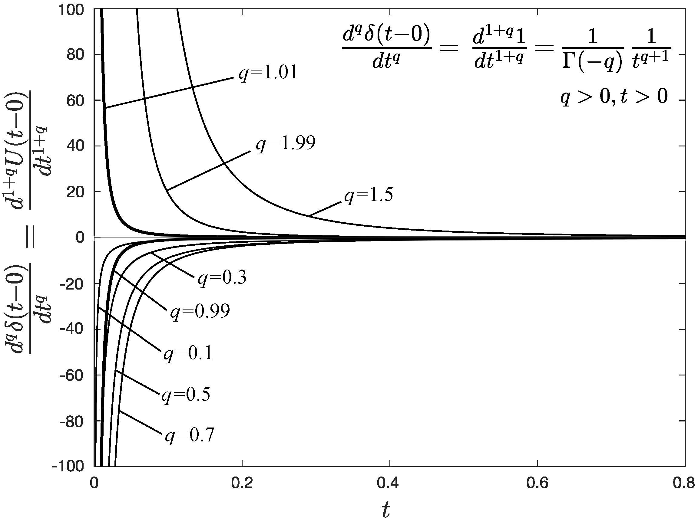
The result of Equation (17) has been presented in [22,25] and has been recently used to study problems in anomalous diffusion [11] and anomalous relaxation [30]. Equation (17) offers the remarkable result that the fractional derivative of the Dirac delta function of any order is finite everywhere other than at ; whereas, the Dirac delta function and its integer-order derivatives are infinite-valued, singular functions that are understood as a monopole, dipole and so on; and we can only interpret them through their mathematical properties as the one given by Equations (6) and (15). Figure 1 plots the fractional derivative of the Dirac delta function at
The result of Equation (18) for is identical to the Gel’fand and Shilov [3] definition of the derivative of the Dirac delta function given by Equation (2), where is the set of positive integers including zero and shows that the fractional derivative of the Dirac delta function with is merely the kernel in the formal definition of the fractional derivative given by Equation (11). Accordingly, in analogy with Equation (12) the fractional derivative of order of a sufficiently differentiable function is
3. The Inverse Laplace Transform of with
The memory function, appearing in Equation (7) of the Scott–Blair (springpot when element expressed by Equation (9) results directly from the definition of the fractional derivative expressed with the Reimann–Liouville integral given by Equation (11). Substitution of Equation (11) into Equation (9) gives
By comparing Equation (20) with Equation (7), the memory function, , of the Scott–Blair element is merely the kernel of the Riemann–Liouville convolution multiplied with the material parameter
where the right-hand side of Equation (21) is from Equation (18). Equation (21) shows that the memory function of the springpot element is the fractional derivative of order of the Dirac delta function as was anticipated by using the argument of physical continuity given that the springpot element interpolates the Hookean spring and the Newtonian dashpot.
In this study we adopt the name “Scott–Blair element” rather than the more restrictive “springpot” element given that the fractional order of differentiation is allowed to take values larger than one. The complex dynamic modulus, , of the Scott–Blair fluid described by Equation (9) with now derives directly from Equation (13)
and its inverse Fourier transform is the memory function, , as indicated by Equation (8). With the introduction of the fractional derivative of the Dirac delta function expressed by Equation (17) or (21), the definition of the memory function given by Equation (8) offers a new (to the best of our knowledge) and useful result regarding the Fourier transform of the function with
In terms of the Laplace variable (see equivalence of Equations (13) and (14)), Equation (23) gives that
where indicates the inverse Laplace transform operator [1,28,29].
When the right-hand side of Equation (23) or (24) is non-zero only when ; otherwise it vanishes because of the poles of the Gamma function when q is zero or any positive integer. The validity of Equation (23) can be confirmed by investigating its limiting cases. For instance, when , then ; and Equation (23) yields that ; which is the correct result. When , Equation (23) yields that . Clearly, the function is not Fourier integrable in the classical sense, yet the result of Equation (23) can be confirmed by evaluating the Fourier transform of in association with the properties of the higher-order derivatives of the Dirac delta function given by Equation (6). By virtue of Equation (6), the Fourier transform of is
therefore, the functions and are Fourier pairs, as indicated by Equation (23).
More generally, for any , Equation (23) yields that = and by virtue of Equation (6), the Fourier transform of is
showing that the functions and are Fourier pairs, which is a special result for of the more general result offered by Equation (23). Consequently, fractional calculus and the memory function of the Scott–Blair element with offer an alternative avenue to reach the Gel’fand and Shilov [3] definition of the Dirac delta function and its integer-order derivatives given by Equation (2). By establishing the inverse Laplace transform of with given by Equation (24) we proceed by examining the inverse Laplace transform of with .
4. The Inverse Laplace Transform of with
The inverse Laplace transform of with is evaluated with the convolution theorem [29]
where given by Equation (24) and = shown in entry (2) of Table 1 [1] which summarizes selective known inverse Laplace transforms of functions with arbitrary power. Accordingly, Equation (27) gives
For the special case where and after using that = [24], Equation (29) reduces to
and the result of Equation (24) is recovered. Equation (30) also reveals the intimate relation between the fractional derivative of the Dirac delta function and the fractional derivative of the power law.
For the special case where , Equation (31) yields and the Gel’fand and Shilov [3] definition of the Dirac delta function given by Equation (2) is recovered. The new results, derived in this paper, on the inverse Laplace transform of irrational functions with arbitrary powers are summarized in Table 2.
5. The Inverse Laplace Transform of with
We start with the known result for the inverse Laplace transform of the function with [25,27]
where is the two-parameter Mittag–Leffler function [31,32,33]
When , Equation (32) reduces to the result of the Laplace transform of the one-parameter Mittag–Leffler function, originally derived by Mittag–Leffler [33]
When , the right-hand side of Equation (32) is known as the Rabotnov function, [11,28,30,34,35]; and Equation (32) yields
Figure 2 plots the function (left) and the function (right) for various values of the parameter . For both functions contract to . When Equation (32) gives
The inverse Laplace transform of with is evaluated with the convolution theorem expressed by Equation (27) where given by Equation (24) and is given by Equation (35). Accordingly, Equation (27) gives
With reference to Equation (11), Equation (37) indicates that is the fractional derivative of order q of the Rabotnov function
For the case where , the exponent q can be expressed as with , and Equation (38) returns the known result given by Equation (32). For the case where , the numerator of the fraction is more powerful than the denominator, and the inverse Laplace transform expressed by Equation (38) is expected to yield a singularity that is manifested with the second parameter of the Mittag–Leffler function , being negative . This embedded singularity in the right-hand side of Equation (38) when is extracted by using the recurrence relation [31,32,33]
By employing the recurrence relation (39) to the right-hand side of Equation (38), then Equation (38) for assumes the expression
Recognizing that according to Equation (18), the first term in the right-hand side of Equation (39) is , the inverse Laplace transform of with can be expressed in the alternative form
in which the singularity has been extracted from the right-hand side of Equation (38), and now the second index of the Mittag–Leffler function appearing in Equation (40) or (41) has been increased to . In the event that remains negative , the Mittag–Leffler function appearing on the right-hand side of Equation (40) or (41) is replaced again by virtue of the recurrence relation (39) and results in
More generally, for any with with and
and all singularities from the Mittag–Leffler function have been extracted. For the special case where Equation (43) gives for with
which is the extension of entry (4) of Table 1 for any . As an example, for Equation (44) is expressed in its dimensionless form
whereas for , Equation (44) yields
Figure 3 plots the results of Equation (45) for 1.3, 1.7, 1.9 and 1.99 together with the results of Equation (46) for 2.01, 2.1, 2.3 and 2.7. When q tends to 2 from below, the curves for approach from below; whereas when q tends to 2 from above, the curves of the inverse Laplace transform approach from above.
6. Summary
In this paper we first show that the memory function, , of the fractional Scott–Blair fluid, with (springpot when is the fractional derivative of the Dirac delta function = with . Given that the memory function is the inverse Fourier transform of the complex dynamic modulus, , in association with that is causal for , we showed that the inverse Laplace transform of for any is the fractional derivative of order q of the Dirac delta function. This new finding in association with the convolution theorem makes possible the calculation of the inverse Laplace transform of when , which is the fractional derivative of order q of the Rabotnov function . The fractional derivative of order of the Rabotnov function produces singularities that are extracted with a finite number of fractional derivatives of the Dirac delta function depending on the strength of the order of differentiation q in association with the recurrence formula of the two-parameter Mittag–Leffler function. The number of singularities, , that need to be extracted when is the lowest integer so that .
Funding
This research received no external funding.
Data Availability Statement
Data is contained within the article.
Conflicts of Interest
The author declares no conflict of interest.
References
- Erdélyi, A. (Ed.) Bateman Manuscript Project, Tables of Integral Transforms Vol I; McGraw-Hill: New York, NY, USA, 1954. [Google Scholar]
- Lighthill, M.J. An Introduction to Fourier Analysis and Generalised Functions; Cambridge University Press: Cambridge, UK, 1958. [Google Scholar]
- Gel’fand, I.M.; Shilov, G.E. Generalized Functions, Vol. 1 Properties and Operations; AMS Chelsea Publishing, An Imprint of the American Mathematical Society: Providence, RI, USA, 1964. [Google Scholar]
- Nutting, P.G. A study of elastic viscous deformation. Proc. Am. Soc. Test. Mater. 1921, 21, 1162–1171. [Google Scholar]
- Gemant, A. A Method of Analyzing Experimental Results Obtained from ElastoViscous Bodies. Physics 1936, 7, 311–317. [Google Scholar] [CrossRef]
- Gemant, A. XLV. On fractional differentials. London Edinb. Dublin Philos. Mag. J. Sci. 1938, 25, 540–549. [Google Scholar] [CrossRef]
- Koeller, R.C. Applications of fractional calculus to the theory of viscoelasticity. J. Appl. Mech. 1984, 51, 299–307. [Google Scholar] [CrossRef]
- Friedrich, C.H.R. Relaxation and retardation functions of the Maxwell model with fractional derivatives. Rheol. Acta 1991, 30, 151–158. [Google Scholar] [CrossRef]
- Schiessel, H.; Metzler, R.; Blumen, A.; Nonnenmacher, T.F. Generalized viscoelastic models: Their fractional equations with solutions. J. Phys. A Math. Gen. 1995, 28, 6567. [Google Scholar] [CrossRef]
- Lutz, E. Fractional Langevin equation. Phys. Rev. E 2001, 64, 051106. [Google Scholar] [CrossRef] [PubMed] [Green Version]
- Makris, N. Viscous-viscoelastic correspondence principle for Brownian motion. Phys. Rev. E 2020, 101, 052139. [Google Scholar] [CrossRef]
- Ozdemir, N.; Derya, A.V.C.I.; Iskender, B.B. The numerical solutions of a two-dimensional space-time Riesz-Caputo fractional diffusion equation. Int. J. Optim. Control. Theor. Appl. IJOCTA 2011, 1, 17–26. [Google Scholar] [CrossRef]
- Povstenko, Y. Solutions to diffusion-wave equation in a body with a spherical cavity under Dirichlet boundary condition. Int. J. Optim. Control. Theor. Appl. IJOCTA 2011, 1, 3–16. [Google Scholar] [CrossRef]
- Yavuz, M.; Özdemir, N. Numerical inverse Laplace homotopy technique for fractional heat equations. Therm. Sci. 2018, 22, 185–194. [Google Scholar] [CrossRef]
- Yavuz, M.; Sene, N. Approximate solutions of the model describing fluid flow using generalized ρ-laplace transform method and heat balance integral method. Axioms 2020, 9, 123. [Google Scholar] [CrossRef]
- Bird, R.B.; Armstrong, R.C.; Hassager, O. Dynamics of Polymeric Liquids. Vol. 1: Fluid Mechanics, 2nd ed.; Wiley: New York, NY, USA, 1987. [Google Scholar]
- Dissado, L.; Hill, R. Memory functions for mechanical relaxation in viscoelastic materials. J. Mater. Sci. 1989, 24, 375–380. [Google Scholar] [CrossRef]
- Giesekus, H. An alternative approach to the linear theory of viscoelasticity and some characteristic effects being distinctive of the type of material. Rheol. Acta 1995, 34, 2–11. [Google Scholar] [CrossRef]
- Scott Blair, G.W. A Survey of General and Applied Rheology; Isaac Pitman & Sons: London, UK, 1944. [Google Scholar]
- Scott Blair, G.W. The role of psychophysics in rheology. J. Colloid Sci. 1947, 2, 21–32. [Google Scholar] [CrossRef]
- Scott Blair, G.W.; Caffyn, J.E., VI. An application of the theory of quasi-properties to the treatment of anomalous strain-stress relations. Lond. Edinb. Dublin Philos. Mag. J. Sci. 1949, 40, 80–94. [Google Scholar] [CrossRef]
- Oldham, K.; Spanier, J. The Fractional Calculus. Mathematics in Science and Engineering; Academic Press Inc.: San Diego, CA, USA, 1974; Volume III. [Google Scholar]
- Samko, S.G.; Kilbas, A.A.; Marichev, O.I. Fractional Integrals and Derivatives; Theory and Applications; Gordon and Breach Science Publishers: Amsterdam, The Netherlands, 1974; Volume 1. [Google Scholar]
- Miller, K.S.; Ross, B. An Introduction to the Fractional Calculus and Fractional Differential Equations; Wiley: New York, NY, USA, 1993. [Google Scholar]
- Podlubny, I. Fractional Differential Equations: An Introduction to Fractional Derivatives, Fractional Differential Equations, to Methods of Their Solution and Some of Their Applications; Elsevier: Amsterdam, The Netherlands, 1998. [Google Scholar]
- Riesz, M. L’intégrale de Riemann-Liouville et le problème de Cauchy. Acta Math. 1949, 81, 1–222. [Google Scholar] [CrossRef]
- Gorenflo, R.; Mainardi, F. Fractional calculus. In Fractals and Fractional Calculus in Continuum Mechanics; Springer: Berlin/Heidelberg, Germany, 1997; pp. 223–276. [Google Scholar]
- Mainardi, F. Fractional Calculus and Waves in Linear Viscoelasticity: An Introduction to Mathematical Models; Imperial College Press-World Scientific: London, UK, 2010. [Google Scholar]
- Le Page, W.R. Complex Variables and the Laplace Transform for Engineers; McGraw-Hill: New York, NY, USA, 1961. [Google Scholar]
- Makris, N.; Efthymiou, E. Time-Response Functions of Fractional-Derivative Rheological Models. Rheol. Acta 2020, 59, 849–873. [Google Scholar] [CrossRef]
- Erdélyi, A. (Ed.) Bateman Manuscript Project, Higher Transcendental Functions Vol III; McGraw-Hill: New York, NY, USA, 1953. [Google Scholar]
- Haubold, H.J.; Mathai, A.M.; Saxena, R.K. Mittag–Leffler functions and their applications. J. Appl. Math. 2011, 2011. [Google Scholar] [CrossRef] [Green Version]
- Gorenflo, R.; Kilbas, A.A.; Mainardi, F.; Rogosin, S.V. Mittag-Leffler Functions, Related Topics and Applications Vol. 2; Springer: Berlin/Heidelberg, Germany, 2014. [Google Scholar]
- Rogosin, S.; Mainardi, F. George William Scott Blair—the pioneer of factional calculus in rheology. arXiv 2014, arXiv:1404.3295. [Google Scholar]
- Rabotnov, Y.N. Elements of Hereditary Solid Mechanics; MIR Publishers: Moscow, Russia, 1980. [Google Scholar]
Figure 1.
Plots of the fractional derivative of the Dirac delta function of order , which are the order derivative of the constant 1 for positive times. The functions are finite everywhere other than the time origin, . Figure 1 shows that the fractional derivatives of the singular Dirac delta function, and these of the constant unit at positive times are expressed with the same family of functions.

Figure 2.
The one-parameter Mittag–Leffler function (left) and the Rabotnov function (right) for various values of the parameter .
Figure 2.
The one-parameter Mittag–Leffler function (left) and the Rabotnov function (right) for various values of the parameter .

Figure 3.
Plots . of = by using Equation (45) for and Equation (46) for . When q tends to 2 from below, the curves for approach from below; whereas when q tends to 2 from above, the curves of the inverse Laplace transform approach from above.


Table 1.
Known inverse Laplace transforms of irrational functions with an arbitrary power.
| (1) | ||
| (2) | ||
| (3) | ||
| (4) | ||
| (5) | ||
| (6) Special case of (5) for β = 1 | ||
| (7) Special case of (5) for α = β | ||
| (8) Special case of (5) for α − β = −1 | ||
| (9) Special case of (5) with 0 < α − β = q < α |
Table 2.
New results on the inverse Laplace transform of irrational functions with arbitrary powers.
Table 2.
New results on the inverse Laplace transform of irrational functions with arbitrary powers.
| (1) | = | |
| (2) | ||
| (3) Extension of entry (9) of Table 1 for | ||
| (4) Special case of (3) for | ||
| (5) General case of (3) for any with | ||
| (6) Special case of (5) for with |
Publisher’s Note: MDPI stays neutral with regard to jurisdictional claims in published maps and institutional affiliations. |
© 2021 by the author. Licensee MDPI, Basel, Switzerland. This article is an open access article distributed under the terms and conditions of the Creative Commons Attribution (CC BY) license (http://creativecommons.org/licenses/by/4.0/).
Share and Cite
MDPI and ACS Style
Makris, N. The Fractional Derivative of the Dirac Delta Function and Additional Results on the Inverse Laplace Transform of Irrational Functions. Fractal Fract. 2021, 5, 18. https://0-doi-org.brum.beds.ac.uk/10.3390/fractalfract5010018
AMA Style
Makris N. The Fractional Derivative of the Dirac Delta Function and Additional Results on the Inverse Laplace Transform of Irrational Functions. Fractal and Fractional. 2021; 5(1):18. https://0-doi-org.brum.beds.ac.uk/10.3390/fractalfract5010018
Chicago/Turabian StyleMakris, Nicos. 2021. "The Fractional Derivative of the Dirac Delta Function and Additional Results on the Inverse Laplace Transform of Irrational Functions" Fractal and Fractional 5, no. 1: 18. https://0-doi-org.brum.beds.ac.uk/10.3390/fractalfract5010018