1. Introduction
Numerical methods have gained considerable attention in many applications, since the exact solution of many problems arising in the models of chemistry, physics, biology, engineering, and many other fields of different sciences is an uphill task. Modeling of these problems leads us to consider a number of physical quantities, representing physical phenomena on a modeling domain. These physical quantities then occur in the model via functions or function derivatives of which for a considerable number of them the Newtonian concept of a derivative satisfies the complexity of the natural occurrences. However, “time’s evolution and changes occurring in some systems do not happen in the same manner after a fixed or constant interval of time and do not follow the same routine as one would expect. For instance, a huge variation can occur in a fraction of a second, causing a major change that may affect the whole system’s state forever” as stated in [
1]. Indeed, it has turned out recently that many of phenomena involved in many branches of chemistry, engineering, biology, ecology, and numerous domains of applied sciences can be described very successfully by models using fractional order differential equations such as acoustic dissipation, viscoelastic systems, mathematical epidemiology, continuous time random walk, and biomedical engineering (see [
1] and references therein). Analytical techniques can not solve most of these models with the conventional integer-order derivative, and models with fractional derivatives appearing in practice. Hence, various methods for the solution of these model problems have been developed and proposed in numerous works, in order to provide an improved description of the phenomenon under investigation. Common numerical methods include finite difference method, finite element method, finite volume method, variational iteration method, adomian or homotopy analysis, wavelet method, etc.
Most recently, for the model problems of chaotic attractors, exhaustive studies were given for the solvability of chaotic fractional systems with 3D four-scroll attractors in [
2], for the Proto–Lorenz system in its chaotic fractional and fractal structure in [
3], and for a new auto-replication in systems of attractors with two and three merged basins of attraction via control in [
4]. To model some symbiosis systems describing commmensalism and predator–prey processes, the Atangana–Baleanu derivative operator was applied in [
5] and a numerical approximation technique was given. Model problems involving a derivative with fractional parameter
and the application to transport-convection differential equations were given in [
1]. In addition, the use of a control parameter to control on processes related to stationary state system, and on relaxation and diffusion, was studied in [
6]. Further, in [
7] a comparative analysis between differential fractional operators including the Atangana–Baleanu derivative and the Caputo–Fabrizio derivative applied to the non-linear Kaup–Kupershmidt equation was given and methods of performing numerical approximations of the solutions were presented. Furthermore, for the numerical solution of fractional Volterra type model problems, recent studies include [
8] that a class of system of nonlinear singular fractional Volterra integro-differential equations was solved by a proposed computational method. In addition, [
9], in which delay-dependent stability switches in fractional differential equations were studied and obtained results were illustrated via a fractional Lotka-Volterra population model. Moreover, [
10] as a biological fractional n-species delayed cooperation model of Lotka–Volterra type was presented. Examples to recent studies on numerical solutions of model problems in fractional structure with both stiff and nonstiff components and the leading-edge model problem can be given to [
11,
12], respectively. A second-order diagonally-implicit-explicit multi-stage integration method was given in [
11] for the solution of problems with both stiff and nonstiff components. An implicit method for numerical solution of singular and stiff initial value problem was developed in [
12]. For the epidemic models latest studies include [
13] that the Crank Nicolson difference scheme and iteration method were used for finding the approximate solution of system of nonlinear observing epidemic model. In addition, [
14], in which a novel and time efficient positivity preserving numerical scheme was designed to find the solution of epidemic model involving a reaction-diffusion system in three dimension.
Apart from rectangular grids, hexagonal grids have been also used to develop finite difference methods for the approximate solution of modeled problems in many applied sciences for more than the half century. These studies include the hexagonal grid methods given in meteorological and oceanographic applications by [
15,
16,
17,
18,
19,
20,
21,
22,
23,
24,
25], of which favorable results were obtained compared with rectangular grids. Hexagonal grids were applied in reservoir simulation in [
26] and it was shown that for seven-point floods, hexagonal grid method provides good numerical accuracy at substantially less computational work than rectangular grid method (five or nine point methods). Hexagonal grids were also used in the simulation of electrical wave phenomena propagated in two dimensional reserved-C type cardiac tissue in [
27]. The exhibited linear and spiral waves were more efficient than similar computation carried out on rectangular finite volume schemes. Furthermore, hexagonal grids were applied to approximate the solution of the first type boundary value problem of the heat equation in [
28,
29,
30], convection-diffusion equation in [
31], and Dirichlet type boundary value problem of the two dimensional Laplace equation in [
32]. In the recent study [
29], the solution of first type boundary value problem of heat equation
on special polygons with interior angles
,
, for
where,
and
f is the heat source by using hexagonal grids has been given. Therein, two implicit methods named as Difference Problem 1 and Difference Problem 2 both on two layers with 14-points have been proposed. It was assumed that the heat source and the initial and boundary functions are given such that the exact solution belongs to the Hölder space
Under this condition, it was proved that the given Difference Problem 1 and Difference Problem 2 converge to the exact solution on the grids with
and
order of accuracy, respectively.
On the other hand, as well as the solution of the modeled problem, the first order partial derivatives of the solution are also essential to determine the rate of change in the solution and the gradients which determines important phenomena in that model. Such as in the electrostatics the first derivatives of electrostatic potential function define electric field. As the calculation of ray tracing in electrostatic fields by the interpolation methods require the specification at each mesh point not only the potential function
but also the gradients
and the mixed derivative
. Motivated by this aim, in this study a second order accurate two stage implicit method for the approximation of the first order derivatives of the solution
of (
1) with respect to the spatial variables
and
on rectangle
D is developed.
The research is organized as follows: In
Section 2, we consider the first type boundary value problem for the heat equation in (
1) on a rectangle
D under the assumption that the heat source and the initial and boundary functions are given such that on
the solution
belongs to the Hölder space
, where
, and
is the closure of
D. In addition, hexagonal grid structure and basic notations are given. Further, at the first stage, a two layer implicit method on hexagonal grids given in [
29] with
order of accuracy, where
h and
are the step sizes in space variables
and
, respectively, and
is the step size in time used to approximate the solution
For the error function when
, we provide a pointwise prior estimation depending on
which is the distance from the current grid point to the surface of
. In
Section 3 and
Section 4, the second stages of the two stage implicit method for the approximation to the first order derivatives of the solution
with respect to the spatial variables
and
are proposed, respectively. It is proved that the constructed implicit schemes at the second stage are unconditionally stable (see Theorem 1 in [
33] which gives the sufficient condition of stability). For
, priory error estimations in maximum norm between the exact derivatives
,
and the obtained corresponding approximate solutions are provided giving
order of accuracy on the hexagonal grids. In
Section 5, a numerical example is constructed to support the theoretical results. We applied incomplete block preconditioning given in [
34] (see also [
35,
36]) for the conjugate gradient method to solve the obtained algebraic systems of linear equations for various values of
r. In
Section 6, conclusions and some remarks are given.
2. First Type Heat Problem and Second Order Accurate
Solution on Hexagonal Grids
Let be a rectangle, where is multiple of and let , , be the sides of D enumerated in anticlockwise direction starting from the side . Further, is the boundary of D and denote by the closure of D. Let with lateral surface more precisely the set of points and also is the closure of . We consider the first type boundary value problem for the two space dimensional heat equation:
BVP(1):
where
is a positive constant. We assume that the heat source function
and the initial and boundary functions
and
, respectively, are given such that the Problems (
2)–(
4) has a unique solution
u belonging to the Hölder class
For the smoothness of solutions of parabolic equations in regions with edges, see [
37] for the Dirichlet and [
38] for the mixed boundary value problems. Let
, with
, where
is positive integer and assign
a hexagonal grid on
with step size
defined as the set of nodes
Let
be the set of nodes on the interior of
and let
=
be the
jth vertex of
D,
Further, let
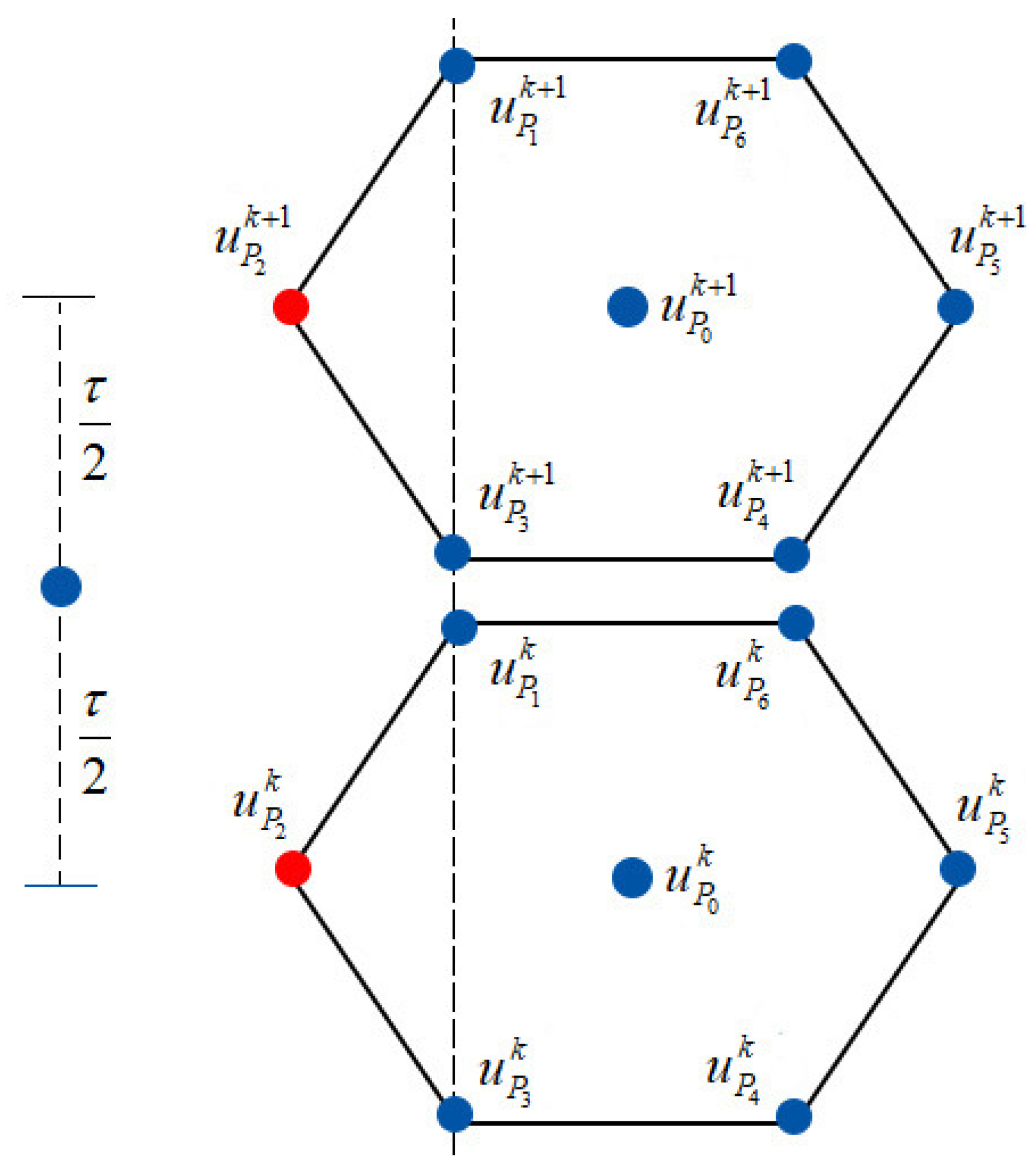
,
denote the set of interior nodes whose distance from the boundary is
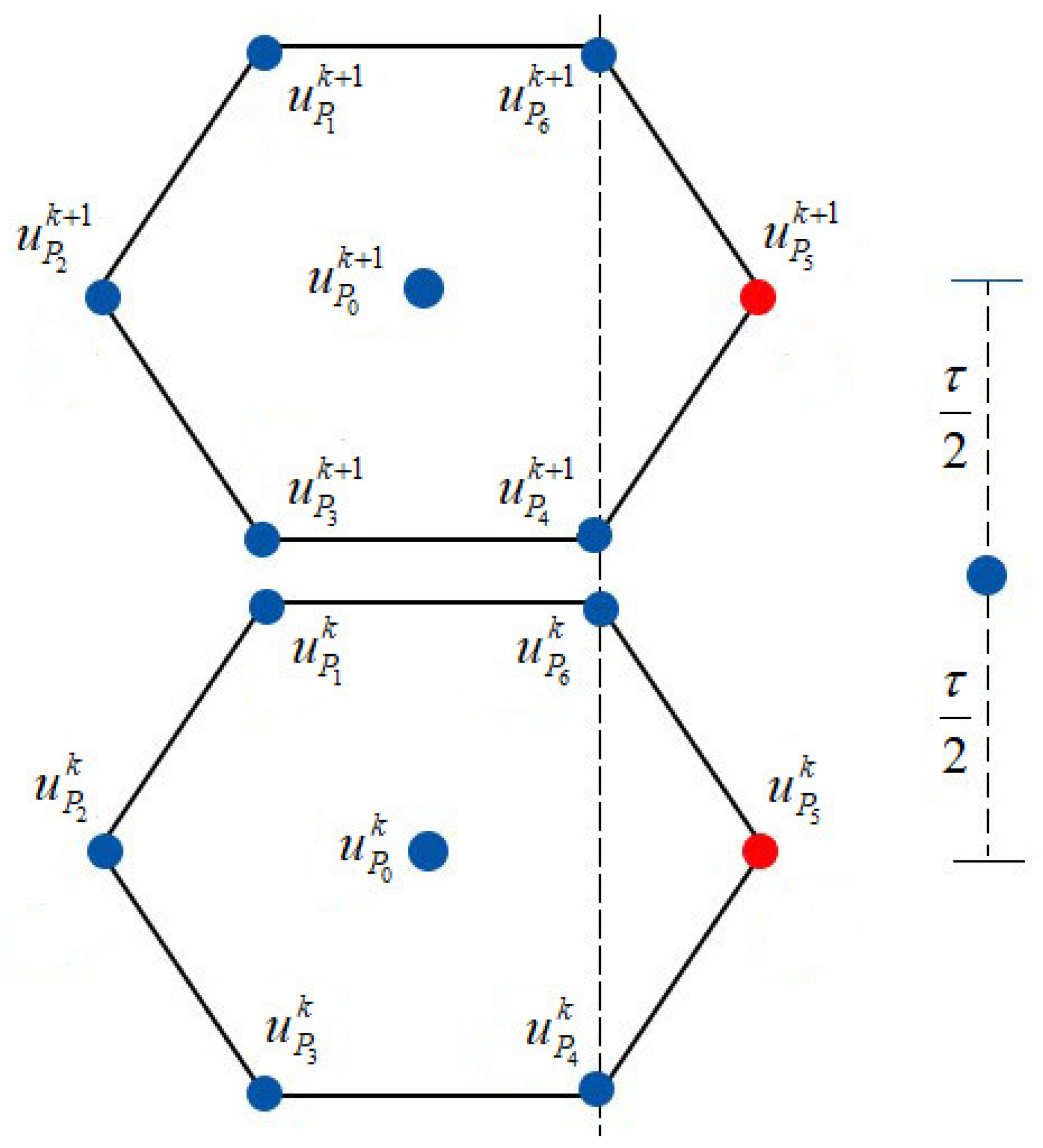
and the hexagon has a left ghost point as shown in
Figure 1 or a right ghost point as presented in
Figure 2, emerging through the left or right side of the rectangle, respectively. We also denote by
and
Next, let
and the set of internal nodes and lateral surface nodes be defined by
respectively. Let
and
and
. In addition,
and
is the closure of
Let
denote the center of the hexagon and
denote the pattern of the hexagon consisting the neighboring points
In addition,
denotes the exact solution at the point
and
denotes the value at the boundary point for the time moment
as follows:
where the value of
if
and
if
as also given in (
21). Analogously, the values
,
and
present the exact solution at the same space coordinates of
,
and
, respectively, but at time level
Further,
and
present the numerical solution at the same space coordinates of
and
for time moments
and
respectively and
and
For the numerical solution of the BVP(1) the following difference problem (named as Difference Problem 1) was given in [
29] which we will consider as the Stage 1
of the two stage implicit method:
Stage 1
for
where
and
By numbering the interior grid points using standard ordering as
the obtained algebraic linear system of equations in matrix form given in [
29] is as follows:
where
are
and
and
The matrix
is the incidence matrix of the neighboring topology with entries unity for the points in the pattern of the hexagon center. In addition,
I is the identity matrix,
is a diagonal matrix with entries
Lemma 1. (a) The matrix A in (22) is a nonsingular M-matrix and is also a symmetric positive definite matrix. (b) and for
Proof. Proof is given in ([
29]). □
From (
10)–(
13) and (
26), the error function
satisfies the following system as given in [
29]
where
and
, and
are the given functions in (
10), (
11), and (
13), respectively.
Pointwise Priory Estimation For the Error Function (27)–(30)
Consider the following systems
for
where
and
are given functions. The algebraic systems (
33)–(
36) and (
37)–(
40) can be written in matrix form
respectively, for every time level
where
A and
B are the matrices given in (
22) and
. We also use the partial order
which means that
is nonpositive and
means that
is nonnegative wherever they present matrices in
or vectors in
.
Lemma 2. Let be the solution of the difference Equation (41) and be the solution of the difference Equation (42). For if for , then Proof. On the basis of Lemma 1,
and if
then
and from (
43) we have
and
Then, assume that
by using induction we have
which gives
,
In addition,
from (
44). Next assume that
by using (
45) and induction gives
Let
and
denote the corresponding sets of grid points. In addition, let
denote the surface of
Theorem 1. For the solution of the problem (27)–(30), the following inequality holds true for whereand u is the exact solution ofBVP(1)and is the distance from the current grid point in to the surface F of Proof. We consider the system
and the majorant functions
in which
satisfy the difference boundary value problem
Therefore, we write the difference problems (
56)–(
59) and (
63)–(
66) for fixed
in matrix form
respectively, where
A and
B are the matrices given in (
22) and
and
Using (
52) and (
56)–(
66) gives
and
and
for
On the basis of Lemma 2, we get
and using that
on
and
on
gives
□
4. Second Order Approximation of on Hexagonal grids
Let the BVP(1) be given, then we use the notations and and denote on and setup the next boundary value problem for
BVP(3):where
L is the operator in (
72) and
is the given function in (
2). We assume that the solution
and take
and
given in (
3),
given in (
4) are the initial and boundary functions, respectively,
is the solution of the difference problem in
Stage 1.
Lemma 5. The following inequality holdsfor where u is the solution of the boundary value Problems (2)–(4) and is the solution of the difference Problems (10)–(13) inStage 1 and and d are as given in (52) and (55), respectively. Proof. Taking into consideration Theorem 1, and using (
51), (
122), and (
123), we have
thus, we obtain (
126). □
Lemma 6. The following inequality is truefor , where and is the solution of the difference problem inStage 1 and and d are as given in (52) and (55), respectively. Proof. From the assumption that the exact solution
at the end points
and
of each line segment
difference formulas (
122) and (
123) give the second order approximation of
, respectively. From the truncation error formula (see [
39]), it follows that
Taking
and using Lemma 5 and the estimation (
127) and (
129) follows (
128). □
We construct the following difference problem for the numerical solution of BVP(3) and denote this stage as
Stage 2
where
, and
are defined by (
122)–(
125) and the operators
, and
are the operators given in (
16)–(
20), respectively. In addition,
From (
130)–(
134) and (
137), we have
where
are defined by (
122)–(
125) and
Let
and
are as given in (
53), (
54), respectively, and
is the constant given in Lemma 6 and
z is the solution of
BVP(3).
Theorem 4. The implicit scheme given inStage 2 is unconditionally stable.
Proof. The obtained algebraic linear system of Equations (
130)–(
134) can be given in matrix form:
for
, where,
are as given in (
22) and
On the basis of the assumption that the exact solution
z of the
BVP(3) belongs to
and using Lemma 1 and induction we get
Therefore, the scheme is unconditionally stable. □
Theorem 5. The solution of the finite difference problem given inStage 2 satisfiesfor where are as given in (146), (147) respectively and is the exact solution ofBVP(3).
Proof. Consider the auxiliary system
where
are defined by (
122)–(
125) and
We take the majorant function
where
The majorant function in (
157) satisfies the difference problem
We write the algebraic system of Equations (
151)–(
154) and (
160)–(
166) for fixed
in matrix form
respectively, where
are as given in (
22) and
. Using (
155)–(
156), we get
and
for
and
Then, on the basis of Lemma 2 follows
,
From
and using (
155), (
156) follows (
150). □
5. Numerical Results
A test problem is constructed of which the exact solution is known to show the efficiency of the proposed two stage implicit method. The rectangle
D is taken as
, and
All the computations are performed using Mathematica in double precision on a personal computer with properties AMD Ryzen 7 1800X Eight Core Processor 3.60GHz. To solve the obtained linear algebraic system of equations, we applied incomplete block-matrix factorization of the block tridiagonal stiffness matrices which are symmetric
—matrices for the all considered pairs of
using two-step iterative method for matrix inversion. Then these incomplete block-matrix factorizations are used as preconditioners for the conjugate gradient method as given in [
34] (see also [
35,
36] ). We use the following notations in tables and figures:
denotes the proposed two stage implicit method on hexagonal grids for the approximation of the derivative
denotes the proposed two stage implicit method on hexagonal grids for the approximation of the derivative .
presents the Central Processing Unit time in seconds ( per time level for the method
presents the Central Processing Unit time in seconds ( per time level for the method
shows the total Central Processing Unit time in seconds required for the solution at by the method
shows the total Central Processing Unit time in seconds required for the solution at by the method
The proposed two stage implicit method for the approximation of the derivatives
are denoted as the methods
and
Additionally, the corresponding solutions are denoted by
, and
, respectively, for
and
where
are positive integers. On the grid points
, which is the closure of
we present the error function
obtained by
and
by
and by
, respectively. In addition, maximum norm of the errors
and
are presented by
and
accordingly. Further, we denote the order of convergence of the approximate solution
to the exact solution
obtained by using the two stage implicit method
by
Analogously, the order of convergence of the approximate solution
to the exact solution
obtained by using the two stage implicit method
is given by
We remark that the values of (
170), (
171) are
showing that the order of convergence of the approximate solution
to the exact solution
and the order of convergence of the approximate solution
to the exact solution
are second order both in the spatial variables
and in time
t, accordingly.
Test Problem:where
are the heat source and exact solution.
Table 1 demonstrates
maximum norm of the errors for
when
, that is
and the order of convergence of
to the exact derivatives
with respect to
h and
obtained by using the constructed two stage implicit method
.
Table 2 shows
maximum norm of the errors for the same pairs of
as in
Table 1 and the order of convergence of
to the exact derivative
with respect to
h and
obtained by using the constructed two stage implicit method
Table 1 and
Table 2 justify the theoretical results given such that the approximate solutions
and
of the proposed method converge to the corresponding exact derivatives
and
with second order both in the spatial variables
and the time variable
t for
.
Table 3 presents the
maximum norm of the errors for
when
that is
and the order of convergence of
to the exact derivative
with respect to
h and
obtained by using the constructed two stage implicit method
.
Table 4 shows the
maximum norm of the errors for the same pairs of
as in
Table 3 and the order of convergence of
to the exact derivative
with respect to
h and
obtained by using the constructed two stage implicit method
Numerical results given in
Table 3 and
Table 4 demonstrate that when
, the approximate solutions
and
of the proposed method also converge with second order both in the spatial variables
and the time variable
t to their corresponding exact derivatives
and
.
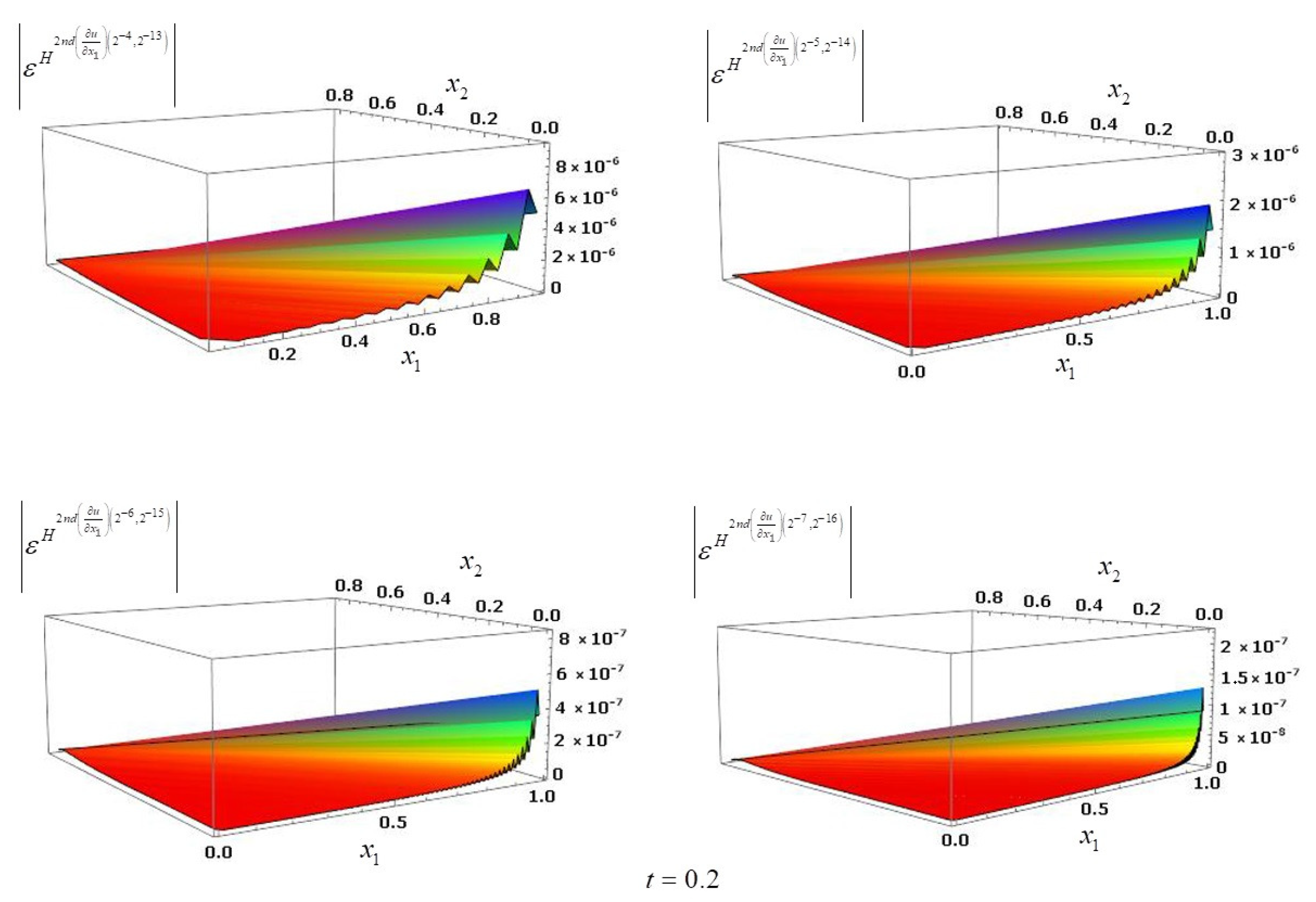
Figure 3 illustrates the absolute error functions
, and
at time moment
obtained by using
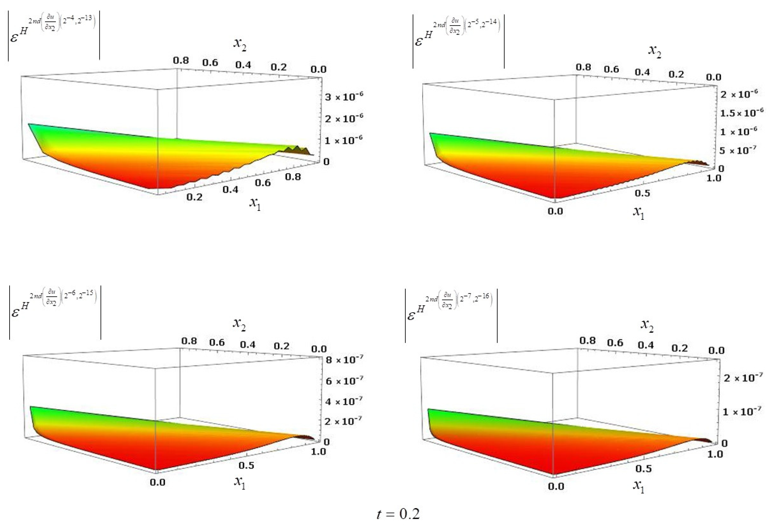
Figure 4 demonstrates the absolute error functions
, and
at time moment
obtained by using
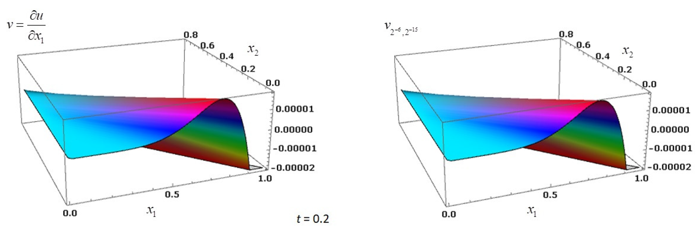
The exact derivative
and the grid function
for
at time moment
obtained by using
are presented in
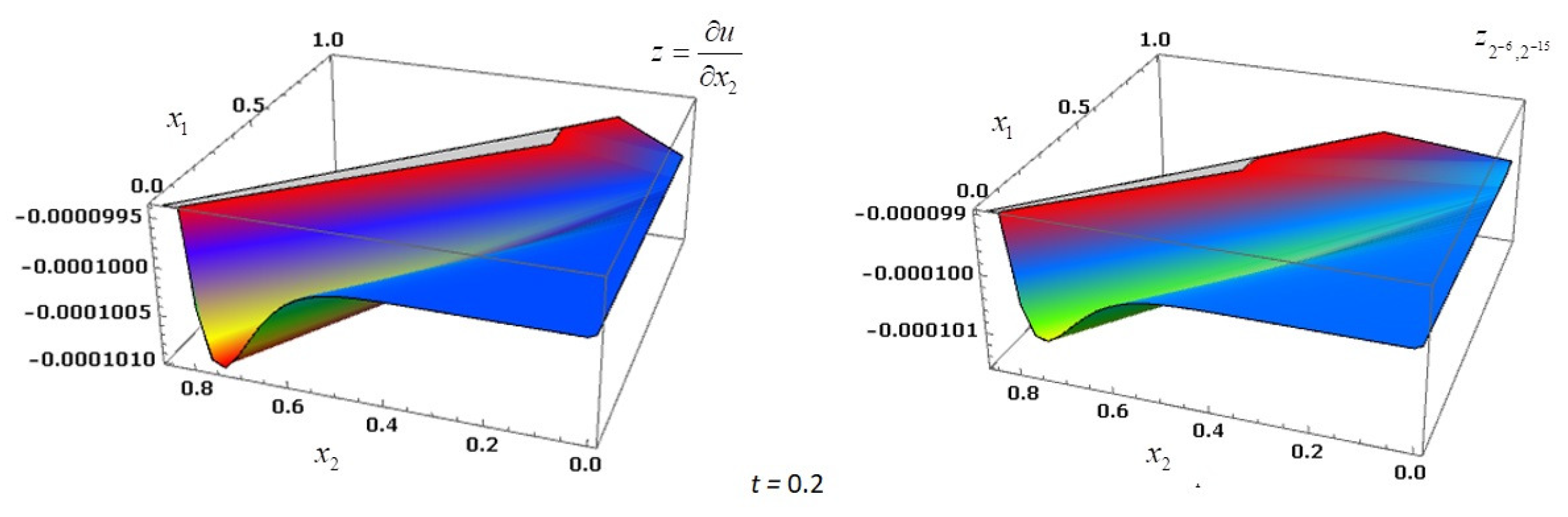
Figure 5. Further,
Figure 6 shows the exact derivative
and grid function
at time moment
obtained by using
Table 5 shows the
maximum norm of the errors for
, and the order of convergence of
to the exact derivative
with respect to
h and
obtained when third order approximations for
are used on
for the
Stage 2 Table 6 shows
,
, maximum norm of the errors for
and the order of convergence of
to the exact derivative
with respect to
h and
obtained when third order approximations for
are used on
for the
Stage 2 Table 7 presents
maximum norm of the errors for
, and the order of convergence of
to the exact derivatives
with respect to
h and
obtained by using the difference formulae (
172), (
173) on
for the
Stage 2.
Table 8 gives
maximum norm of the errors for
, and the order of convergence of
to the exact derivative
with respect to
h and
obtained by using the difference formulae (
174), (
175) on
for the
Stage 2 Numerical results given in
Table 5,
Table 6,
Table 7 and
Table 8 demonstrate that the approximate solution
and
of the proposed method converges to the corresponding exact derivatives
and
with second order both in the spatial variables
and the time variable
t with better error ratios.


