5G Poor and Rich Novel Control Scheme Based Load Frequency Regulation of a Two-Area System with 100% Renewables in Africa


Electromechanics Engineering Department, Faculty of Engineering, Heliopolis University, Cairo 11785, Egypt
Fractal Fract. 2021, 5(1), 2; https://0-doi-org.brum.beds.ac.uk/10.3390/fractalfract5010002
Submission received: 14 November 2020
/
Revised: 14 December 2020
/
Accepted: 21 December 2020
/
Published: 23 December 2020
(This article belongs to the Special Issue Fractional-Order Circuits and Systems)
Abstract
:Remote farms in Africa are cultivated lands planned for 100% sustainable energy and organic agriculture in the future. This paper presents the load frequency control of a two-area power system feeding those farms. The power system is supplied by renewable technologies and storage facilities only which are photovoltaics, biogas, biodiesel, solar thermal, battery storage and flywheel storage systems. Each of those facilities has 150-kW capacity. This paper presents a model for each renewable energy technology and energy storage facility. The frequency is controlled by using a novel non-linear fractional order proportional integral derivative control scheme (NFOPID). The novel scheme is compared to a non-linear PID controller (NPID), fractional order PID controller (FOPID), and conventional PID. The effect of the different degradation factors related to the communication infrastructure, such as the time delay and packet loss, are modeled and simulated to assess the controlled system performance. A new cost function is presented in this research. The four controllers are tuned by novel poor and rich optimization (PRO) algorithm at different operating conditions. PRO controller design is compared to other state of the art techniques in this paper. The results show that the PRO design for a novel NFOPID controller has a promising future in load frequency control considering communication delays and packet loss. The simulation and optimization are applied on MATLAB/SIMULINK 2017a environment.
1. Introduction
Developing countries worldwide are planning to face climate change through increasing the penetration level of organic agriculture and sustainable energy. With smart grid technologies in terms of online monitoring, along with the real time control and self-healing of microgrids, the existence of electricity from 100% sustainable energies has become applicable [1].
The under frequency and over frequency are the two common reasons for the blackout of a microgrid or a power grid. The frequency control of the microgrids especially those with high penetration level of renewables is very important in terms of security and reliability [2].
In recent years, the penetration level of renewables has continuously increased worldwide, especially wind and PV generating systems. In 2020, the penetration level of renewables in Iceland reached 100%, some other countries achieved more than 95% like Norway and Costa Rica, while Canada, Kenya, and Brazil achieved more than 70%. The penetration level of renewables worldwide in 2020 reached 23% [3,4,5]. With this continuous increase of those technologies, power system behavior has become more complex [6].
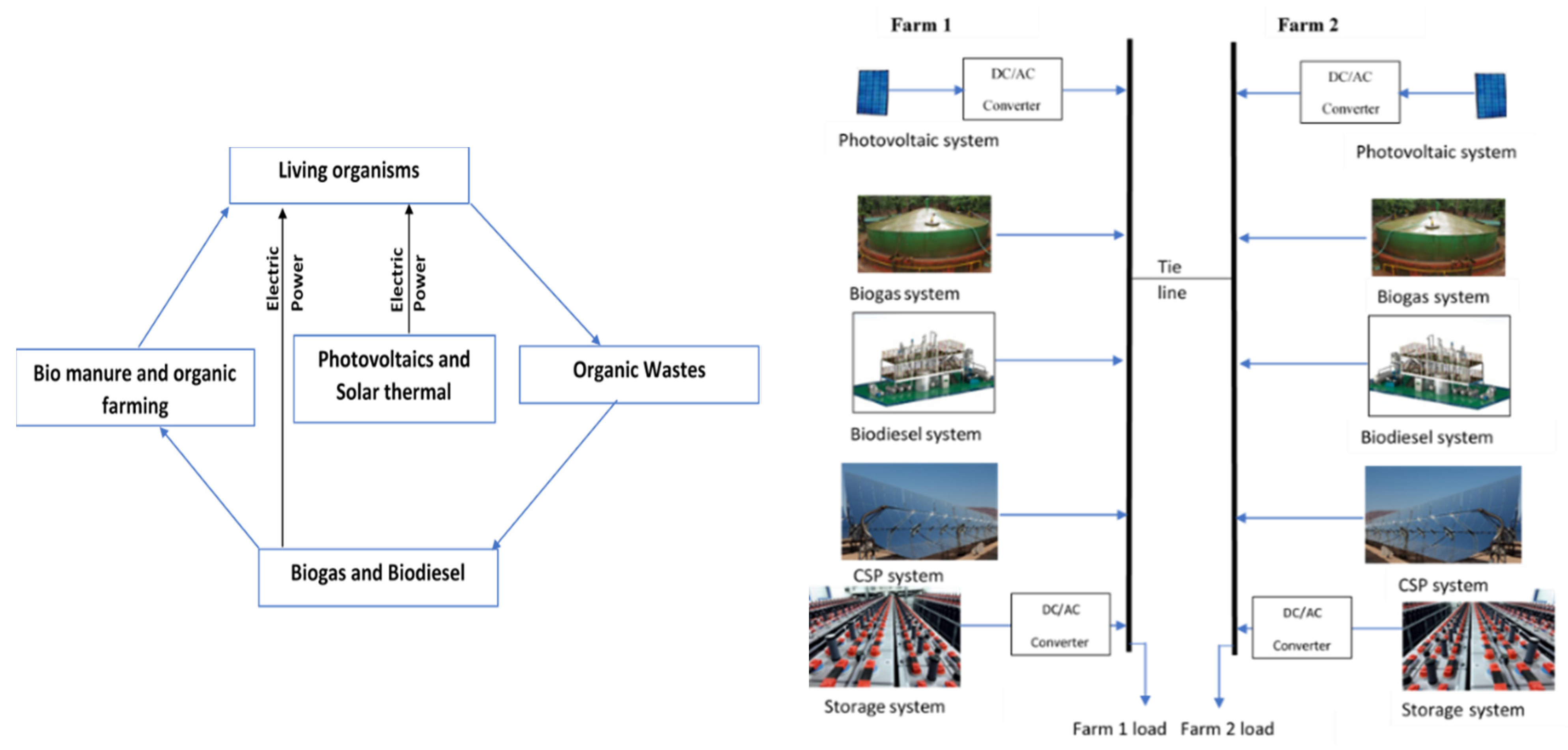
The energy food nexus (EFN) is one of the proposed solutions to achieve sustainable development goals and face climate change. EFN can be achieved through integration of organic agriculture and sustainable energy in remote farms [7]. The developing countries worldwide can achieve 100% renewable power generation target by using bioenergy, especially in remote villages of those countries. Renewable technologies such as photovoltaics, solar thermal, and wind turbines are not that reliable as generators due to the stochastic nature of sun and wind. A diesel generator is always used with the renewable resources, which has a high carbon dioxide emission [8]. In this paper, we replace the conventional diesel generator with biodiesel and biogas generators which have less emissions. The main idea is illustrated in Figure 1.
Biogas is a mixture of gases produced in absence of oxygen due to break down of manure, plant, farming wastes or even sewage. It can be produced through the fermentation of biodegradable materials or anaerobic digestion with anaerobic organisms inside biodigester [8]. It consists of methane (CH4), carbon dioxide (CO2), and aphoristic galore of hydrogen sulphide (H2S). CH4 and CO can be combusted and then can produce electricity through a turbine generator (GTG) [9,10]. This is modelled as a biogas-turbine generator (BGTG) in this action.
Biodiesel is a carbon neutral eco-friendly alternative to fossil diesel. Biodiesel is produced from vegetable oil, animal fats or tallow through transesterification. The transesterification process is the chemical reaction of a triglyceride (fat/oil) with an alcohol to form esters and glycerol. During the esterification process, the triglyceride is reacted with alcohol in the presence of a catalyst, usually a strong alkaline like sodium hydroxide then biodiesel can be produced [11]. The biodiesel is used in an engine to instantaneously produce demanded electricity like the conventional diesel generator but with special requirements [12,13].
Various control schemes were used to control the frequency of interconnected systems. The controller’s applied technology started with a P controller followed by PI and PID controllers. Non-integer differentiation and integration has been studied over four centuries by many scientists. In the 18th century, Euler and Lagrange were the first to introduce a theoretical contribution. In the 19th century, Liouville reached a function expansion in a series of exponentials and definition of nth order derivative, while Riemann presented the definite integral applicable to power series with non-integer exponents. Grunwald and Krug unified the results of Liouville and Riemann [14,15]. The non-integer derivatives and integrals are key points to improve the performance of various applications. The FOPID has proved its existence either in research or industry by academics or researchers. The appearance of fractional order controller may be attributed to Oustaloup, who introduced and demonstrated the superiority of the Commande Robuste dOrdre Non Entier (CRONE) controller [14,15]. Many applications in load frequency control have been applied using CRONE FOPID, and in comparison with the PID controller, the FOPID demonstrated better performance over the PID controller. The reason behind that is the presence of five variables instead of only three, however optimal tuning of the five variables is more complex.
In [14], a comparison between the PID controller, Hꝏ controllers, and FOPID controller was presented to control the frequency of hybrid power system. The system achieved the best performance using the FOPID controller.
In [16], a frequency control technique was presented in a 100% sustainable energy marine microgrid. The microgrid includes a wind, tidal, and wave hybrid energy system. The research depends on the injection of power from tidal energy through non-linear fractional integrator supplementary control to regulate the frequency deviation at zero for different operating conditions.
In [8], a single area microgrid model, which includes photovoltaics, biogas and biodiesel generating systems, was presented. The model was controlled by conventional P, PI, PD, and PID controllers designed using the grasshopper method. The results show that the PID controller leads the system to the best performance. The study doesn’t consider the communication delays.
Many researchers tracked different optimization techniques in load frequency control aiming for better performance as with the genetic algorithm [14]. In [17], the particle swarm algorithm (PSO) is presented, in [18] the grasshopper optimization algorithm (GOZ) is presented, and in [19] socio evolution & learning optimization (SELO) is presented. Poor and rich optimization algorithm (PRO) was presented for the first time in [20] by Moosavi and Bardsiri as a novel human meta-population approach for solving engineering optimization problems.
In microgrids, transmitting information between the distributed components like PMUs, controllers, and actuators has become a hot topic for research nowadays. The main advantages of modern communication techniques are easy installation and expansion, high speed, and low cost [21]. Many studies have assessed the performance of the communication systems in power systems such as Can bus [22], Ethernet [23], ZigBee [24], WiMAX (IEEE 802.16) [25], and Wi-Fi (IEEE 802.11) [26]. In fact, the main factors in communication delays which may affect the system performance negatively are network-induced delays and data packet dropouts. Those two factors should be considered in controller design to ensure reliable performance. The Internet of Things-based 5G is applied in [27] for transferring the measurement signals of multiple distributed generators to a control center.
The main contributions of this research are:
- Integration of sustainable energy with organic agriculture to reach 100% renewable energy microgrid as a form of EF nexus.
- Consideration of 5G communication and PMUs placement in load frequency control of the two interconnected microgrids.
- The novel PRO algorithm is applied to tune the parameters of different control schemes including NFOPID controller as the newest scheme in load frequency control. A comparison between the new algorithm and state of the art algorithms is presented. A new objective function to design the controllers is also presented in this study.
- The effect of network degradation (time delays and packet losses) is considered in the comparison between different control schemes.
The paper is organized as follows. Section 2 provides the system description. Section 3 presents system modeling while Section 4 illustrates the configuration of the novel NFOPID controller. Section 5 illustrates how the controllers are designed in MATLAB using novel PRO. Section 6 illustrates how the communication is configured in the system. Section 7 presents the simulation results and Section 8 summarizes the main conclusions of the research.
2. System Description
Africa is famous for its agricultural land and solar energy. The EFN is now a hot topic to achieve sustainable development goals in terms of zero hunger and affordable clean energy. Solar and bioenergy technologies can highly contribute to the EF nexus in terms of food prices, economic growth, energy security, deforestation, land use, and climate change [28]. Many previous experiences in Africa proved that biomass could contribute to food security. The production of bioenergy in integrated food–energy systems is one such approach. Intercropping Gliricidia (a fast-growing, nitrogen-fixing leguminous tree) with maize in Malawi or with coconut in Sri-Lanka is substantially improving yields of agricultural products while also providing sustainable bioenergy feedstock. Such an integrated food-energy industry can enhance food production and nutrition security, improve livelihoods, conserve the environment, and advance economic growth [28].
In [1] and [8], a microgrid integrating bioenergy with solar energy technologies to form a single area microgrid. In this research, it was assumed that we have two similar organic farms in Egypt using sustainable technologies for energy generation and agriculture as illustrated in Figure 1. They are isolated from the grid and interconnected with each other. The two-area power system described in this paper is fed by technologies powered by renewable resources. The power system integrates the solar energy with the bioenergy. The solar energy technologies used are photovoltaics and solar thermal power generation systems. The bioenergy technologies are the biogas and biodiesel technologies. Two energy storage facilities are used: battery and flywheel systems. Each technology or facility has a nominal power 150 kW. The SIMULINK model is illustrated in Figure 2.
Each area includes three controllers, the first one is assigned for both biodiesel and biogas. The second controller controls the flywheel storage system and the third one controls battery storage system. Each controller is responsible for actuating the technology responding to the frequency deviations. In this research, the three controllers are from the same type at each simulation running time.
3. System Modelling
This section presents how each renewable technology, energy storage facility, and power system are modeled and simulated in MATLAB [1,8].
3.1. Photovoltaic Power Generation Model:
The photovoltaic power generators transform the sunlight directly to electricity through crystalline or thin film panels. In this study, it was assumed that the photovoltaic generating system is working without wiring losses. The power extracted from the photovoltaic system can be formulated as (1) [1,8].
where is the photovoltaic system output power Watt, I is the isolation in Watt/m2, is the photovoltaic park field area in m2, is the electricity conversion from sunlight efficiency, and is the ambient temperature. In this paper, it was assumed that linearly increase with . The transfer function of the photovoltaic generating system can be modeled as (2) [1,8].
where is the time constant of the photovoltaic generating unit.
3.2. Solar Thermal Generating System:
Solar thermal systems are widely used nowadays to produce either heat or electrical energy or even both. The solar thermal power technologies are parabolic trough collectors, parabolic dish, central receiver, and linear Fresnel. Those technologies are mainly depending on reflecting the heat of the sun to a point or a line to heat a medium (usually oil or molten salt because they have high boiling points) to a high temperature. The highly heated mediums exchange the temperature with water to produce steam which can rotate a turbine then creates electrical energy.
The solar thermal system has a transfer function illustrated in (3) [1].
where is the charging time constant of the turbine, is the gain of the turbine, is the solar collector time constant, and is the solar collector gain.
3.3. Biogas Generating System
Biogas can be used for power production. It is mainly extracted from animal wastes. The biogas power generating system includes gas valve actuator, speed governor, turbine, fuel system, and combustor. The output power extracted from the biogas generating system is mainly depending on the gas inlet valve control action, governor action and turbine /combustor actions. The transfer function ( can be written as illustrated in (4) [1,8,10].
where , , , , , and are combustion reaction delay, biogas delay, lead time, lag time, valve actuator and discharge time constants of biogas generating system, respectively. is the change in biogas power and represents the contribution of biogas with respect to the bioenergy controller signal.
3.4. Biodiesel Generating System
Through transesterification, biodiesel can be extracted from energy crops with properties like that of the conventional diesel. The rate of work done by the biodiesel generating system is illustrated in (5) [1,8].
where , , and θ are the universal gas constant, the instantaneous temperature in Kelvin at any crank angle θ, the length of connecting rod in m, the stroke length in m, the displacement volume in m3, and the angular displacement with respect to bottom dead center in degree of the biodiesel generating system respectively [1,11].
The power extracted from biodiesel generating system is mainly dependent on the biodiesel inlet valve action and the internal combustion (IC) engine action. The transfer function ( can be written as illustrated in (6) [1,8].
where , and are the valve gain, valve actuator delay, engine gain and time constants of biodiesel generating system respectively. represents the contribution of biodiesel with respect to the bioenergy controller signal and is the change in biodiesel power.
3.5. Energy Storage Facilities
The energy storage systems have vital role in high penetration level of renewables power systems due to weather uncertainty. During the presence of surplus generated power from renewables, the storage systems absorb energy and during the presence of deficit power, the storage systems release power to feed the load requirements.
In this work, there are two energy storage technologies used Battery and flywheel storage systems. The transfer function of battery technologies is illustrated in (7) and a flywheel storage system is illustrated in (8) [1].
where and are gain and time constant of battery storage system, respectively, while and are gain and time constant of flywheel storage system, respectively.
3.6. Power System Dynamics Model
Since the system consists of four renewable technologies generating units in addition to two storage facilities. The active power equation of each area can be written as shown in (9).
where and are the power generated by photovoltaic, solar thermal, biogas and biodiesel generating units respectively while and are the power generated/absorbed from/by the battery and flywheel storage systems respectively. is the power absorbed by the demand, is the change in electrical power of the area and is the incremental change of tie line power. represents the synchronized power while and represents the change in electrical frequencies of the first and second farms microgrids respectively.
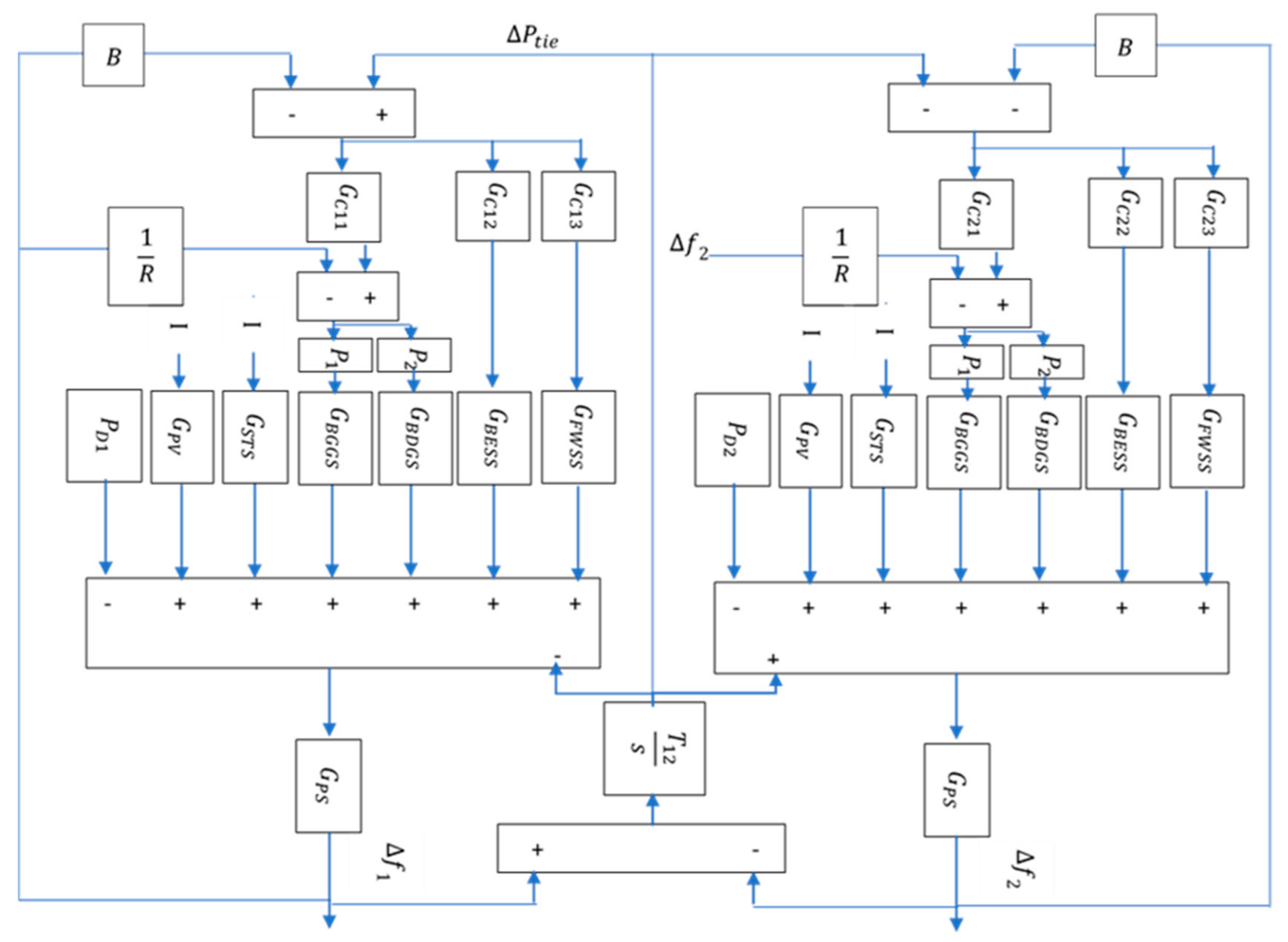
The overall generator dynamics for the whole system can be illustrated in the transfer function illustrated in (10).
where is the change in frequency, is the damping constant of the power system, and is the equivalent inertia constant of each microgrid. B represents the frequency bias factor while is the speed regulation. All the system parameters are shown in Table 1.
4. Control Schemes
4.1. Fractional Order Calculus
Many definitions have been used to describe the fractional order calculus. The most famous definitions are:
The previously mentioned definitions are all inapplicable in terms of real-time control applications [30]. Oustaloup in [31] created an approximation for the fractional order derivative which enabled different researchers from different fields to apply optimal tuning of the five parameters of the FOPID, such as [32,33]. From the practical point of view, the approximation made by Oustaloup is widely used in various applications using CRONE block in MATLAB/SIMULINK, such as:
- i.
- Robotics control [34]: Sara et al. presented FOPID control of a master slave robotics system.
- ii.
- Power system control [35]: Pahadasingh et al. presented FOPID load frequency control of four different thermal areas including HVDC.
- iii.
- DC machines control [36]: Mehra et al. presented FOPID speed control of DC machines.
- iv.
- Photovoltaics system maximum power point tracking [37]: Jeba et al. presented maximum power point tracking of a photovoltaics system using an FOPID controller.
In this work, Oustaloup approximation is used to model the integral and derivative parts of the fractional order PID. The mathematical approximation for is illustrated in Equations (11)–(13).
where is the maximum value for frequency approximation and assumed to be 10,000 in this study while is the minimum value for frequency approximation and assumed to be −10,000 in this study. is the order of the recursive filter proposed by Oustaloup, and in this study N is assumed to be 4. is a pole while is a zero.
4.2. NFOPID Control Scheme
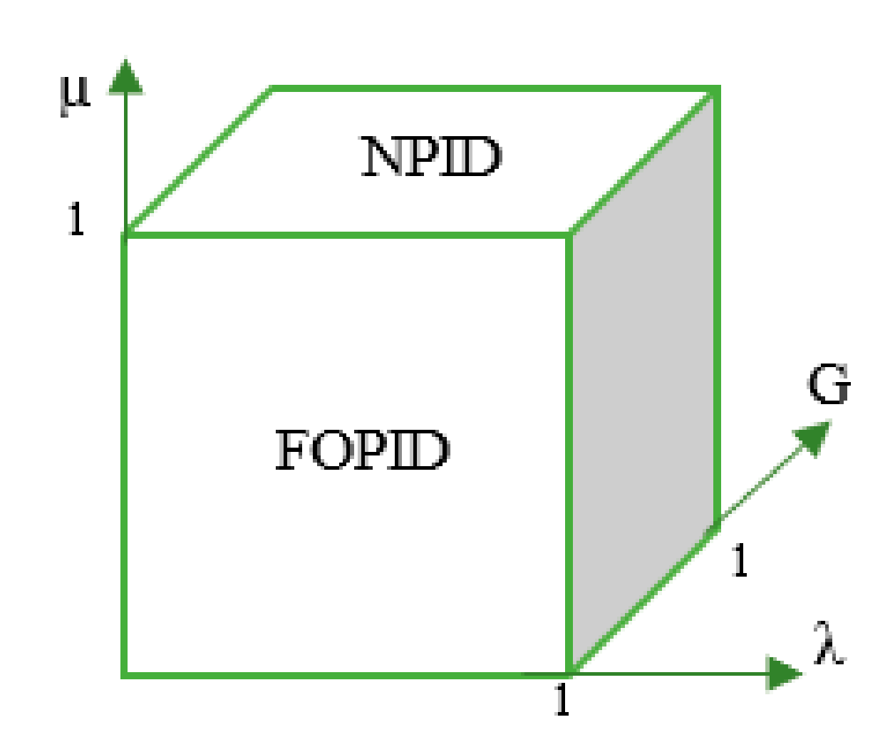
NFOPID is a novel control scheme, includes the advantages of both FOPID and NPID. NFOPID has 6 variables which are:
- Proportional gain (KP)
- Integral gain (KI)
- Derivative gain (KD)
- Integral power (λ)
- Derivative power (µ)
- Non-linearity gain (G)
The six variables give a chance for the novel controller to track a certain reference with better performance in terms of settling time, maximum overshoot, minimum overshoot, peak time, and steady-state error better than state of the art control schemes. The control action of PID, NPID, FOPID, and NFOPID are shown in (14)–(17) [1]. The controller modes of operation and configuration are shown in Figure 3 and Figure 4, respectively.
G ranges between 0 and 1, if G = 0, the NPID controller turns to conventional PID controller.
5. Controllers Design
5.1. Optimization Problem Definition
The design of the controllers will be performed for the operation condition using different optimization techniques which are: PRO [20], SELO [19], GOZ [18], and PSO [17]. Then, the rest of the operating conditions are performed using PRO only. The design is made using MATLAB/SIMULINK. A novel objective function-based optimization problem is described as follows:
- Objective Function (): Minimization of the sum of deviations derivatives multiplied by time.
- Variables: controllers’ parameters.
- Constraints: G, λ, and µ limits.
The controller parameters differ from controller to another. In NPID controller, there are 4 variables (G, KP, KI and KD) and the constraint considered in its design is 0 ≤ G ≤ 1 only. In FOPID, there are 5 variables (KP, KI, KD, λ and µ) and the constraints considered are 0 ≤ λ ≤ 1 and 0 ≤ µ ≤ 1 only. In NFOPID controller the six parameters are the variables and the limits of G, λ, and µ are considered as constraints.
5.2. Poor and Rich Optimization Algorithm
In 2019, Moosavi and Bardsiri [20] established a new multi-population algorithm. The algorithm inspired by the efforts of poor and rich people to increase their wealth or improve their economic status. The PRO algorithm can be described in two points as follows:
- Every poor member is trying to improve his status by learning from the rich.
- Every rich member is trying to widen the gap with poor members by monitoring and acquiring further wealth.
A random design for the first population is made to include rich and poor as a uniform vector. Based on the fitness function, this population will be rearranged such that the first part will include the best rich group values and the second part will include the best poor group values. The flow chart of the poor and rich optimization algorithm is shown in Figure 5.
- Initial population:
The initial population includes two subpopulations, first one for the rich and the other for the poor. It is randomly selected and uniformly distributed, sorted in ascending order based on the fitness function’s response. Normally, all the rich subpopulation members are higher than those of the poor.
where is the size of the main population while the size of subpopulations of reach and poor are and .
- Position update
After each iteration, the position of each population member is changed. The change rich subpopulation member is illustrated in (20) while the change poor subpopulation member is defined in (21).
where and are the new value and the present value of ith position of the rich subpopulation. is the current position of the best poor subpopulation member and w is the class gap member. and are the new value and the current value of ith position of the poor subpopulation while r is the pattern improvement. The pattern is defined in (22).
where , and are the best, mean and worst member positions of the rich subpopulation.
- Mutation
The mutation process is defined in (23) and (24).
- Forming new population after each iteration
There are four populations after any iteration, those populations are evaluated by the fitness function and combined at the end of each iteration. The four populations are the old population of the poor, old population of the rich, new population of the poor and new population of the rich.
5.3. Indicators
Integral absolute error (IAE) and integral time absolute error (ITAE) are employed as indicators to compare between different optimization techniques and controllers.
6. Monitoring and Communication Network
In the smart grid era, communications in power systems play the most important role. The SCADA systems which were previously used to monitor the power systems and microgrids but with the point to point limitations. PMUs are now widely used in different Transmission and distributions systems. In this work, PMU is selected to perform system monitoring for load frequency control. The communication facility is selected to be 5G considering the network degradation factors. Figure 6 shows the whole system including communication network. There are two types of delay in the communication system, the first type is mainly related to the data transferred from PMUs to controllers ΓPC and the second type is for the data transferred between controllers and actuators ΓCA. The second source of disturbance that has a significant impact on network degradation lies at the packet loss [23,38]. The degradation factor exists in the forward and feedback channels of the wireless networks. In this work, the degradation factor is modeled as a two-state switch. A Bernoulli distribution [23] with the stochastic variable is considered in this work, defined as illustrated in (23).
= 0 indicates the occurrence of packet loss, = 1 indicates to no packet loss, and 0 < < 1 is the specified packet loss probability.
In this work the PMUs are located to measure the following:
- Change in area 1 frequency ),
- Change in area 2 frequency ),
- Area 1 control error (ACE1),
- Area 2 control error (ACE2).
The 5G transmitters and receivers are located at
- Change in area 1 frequency ) (transmitter),
- Change in area 2 frequency () (transmitter),
- Area 1 control error (ACE1) (transmitter).
- Area 1 Bioenergy controller input (ACE1) (receiver)
- Area 1 Battery controller input (ACE1) (receiver)
- Area 1 flywheel controller input (ACE1) (receiver)
- Area 2 control error (ACE2) (transmitter)
- Area 2 Bioenergy controller input (ACE2) (receiver)
- Area 2 Battery controller input (ACE2) (receiver)
- Area 2 flywheel controller input (ACE2) (receiver)
7. Simulation Results
7.1. Test 1: Comparison between Four Optimization Techniques
The system is subjected to 6% increase in area 1 demand and 3% change in area 2 demand at night (there’s no sun). The system is controlled through PID controllers only in this test. The results in Figure 7 and Figure 8 and Table 2 show that PRO has better performance over other optimization techniques.
7.2. Test 2: Comparison between Four Control Schemes at Night
The system is subjected to 20% increase in area 1 demand and 12% increase in area 2 demand at night (there’s no sun). Comparison between four control schemes is presented in Figure 9 and Figure 10, and Table 3. The controllers are designed using PRO algorithm. The results show that bioenergy contributes to demand power variations better than storage. The results also prove that the NFOPID drives the system to better performance than other control schemes.
7.3. Test 3: Comparison between Four Control Schemes at Real Case
Areas 1 and 2 are subjected to real change in Egyptian radiation and demand as illustrated in Figure 10. The data were measured at SEKEM farm in Belbeis, Egypt [39]. Both areas have the same performance. Comparison between the four control schemes is presented in Figure 11 and Table 4. The control schemes parameters are the same in Test 2. The results show that the novel NFOPID has better performance than other control schemes.
7.4. Test 4: Comparison between Four Control Schemes at Real Case Considering Time Delay
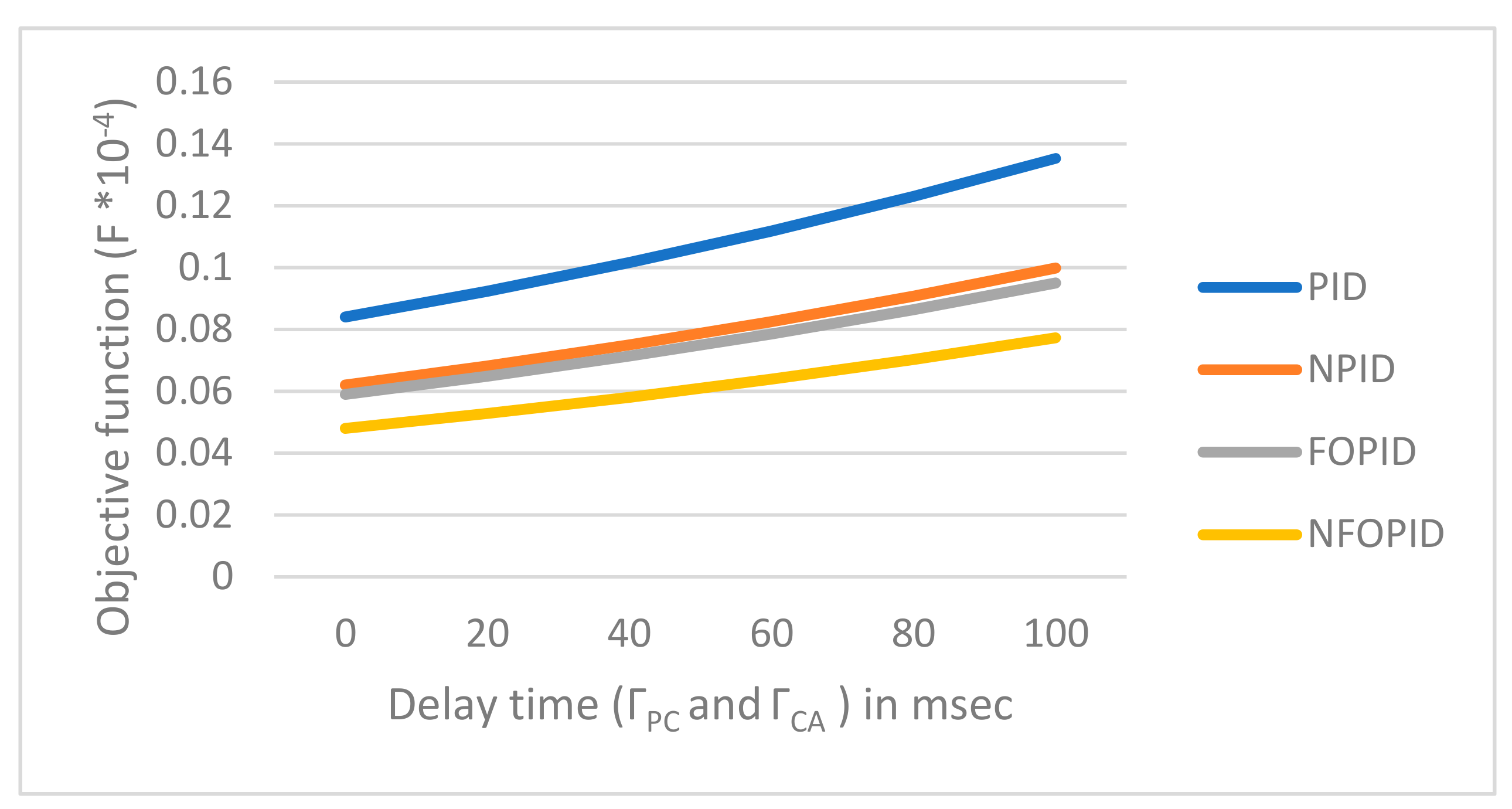
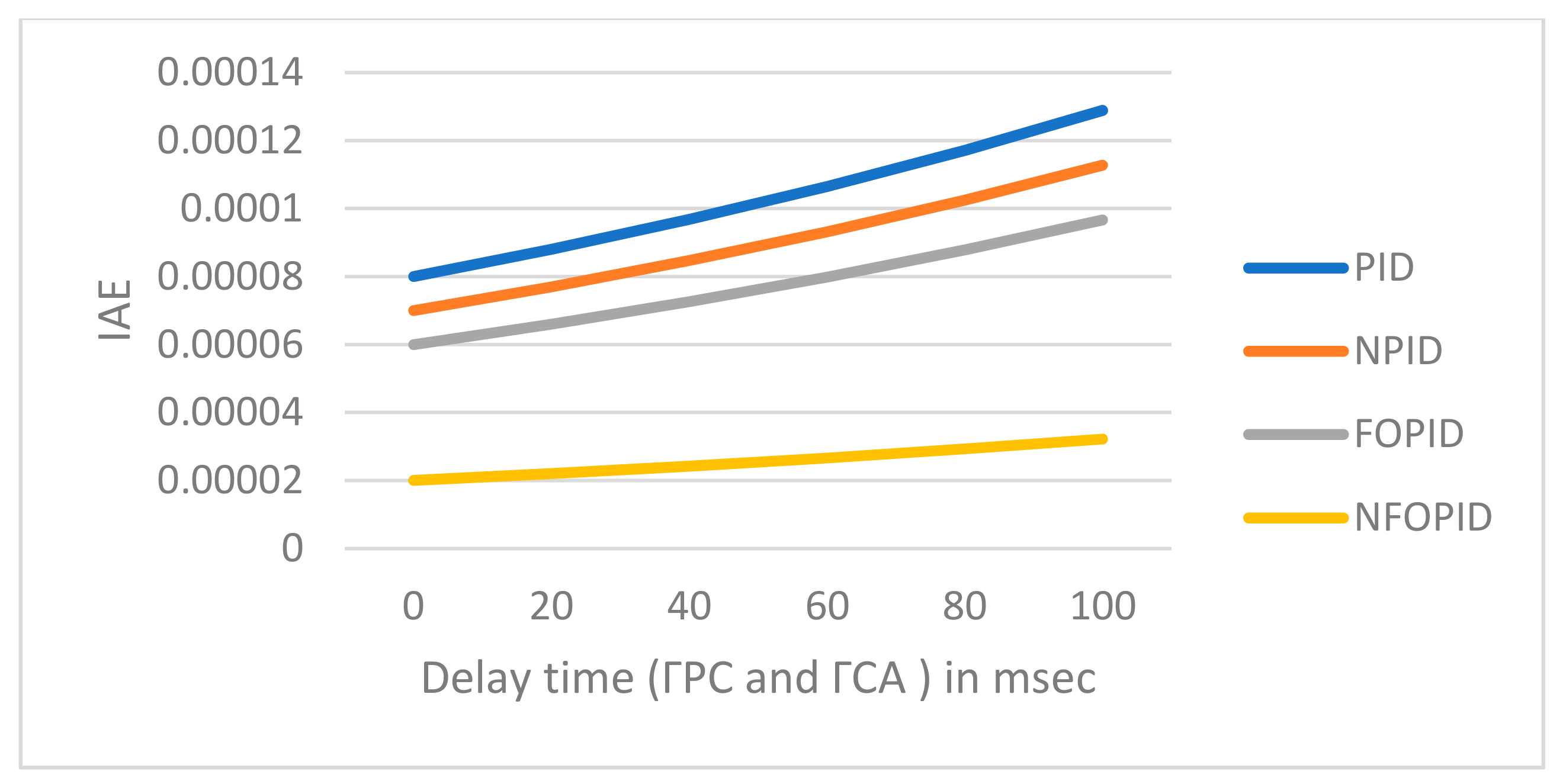
The effect of time delay from sensor to controller and from controller to actuator (ΓPC and ΓCA) on the system using different control schemes are considered with range [0 ms, 100 ms]. In this test the packet loss is assumed to be constant with value . the test is applied on the same operating condition of Test 3 (real case). Figure 12, Figure 13 and Figure 14 show the effect of time delay on the objective function, ITAE, and IAE.
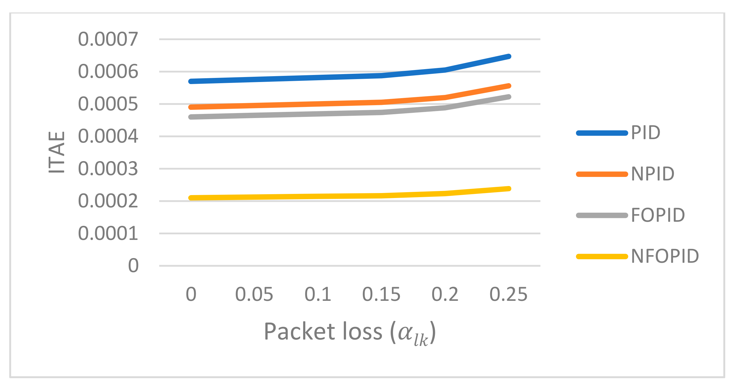
7.5. Test 5: Comparison between Four Control Schemes at Real Case Considering Packet Loss
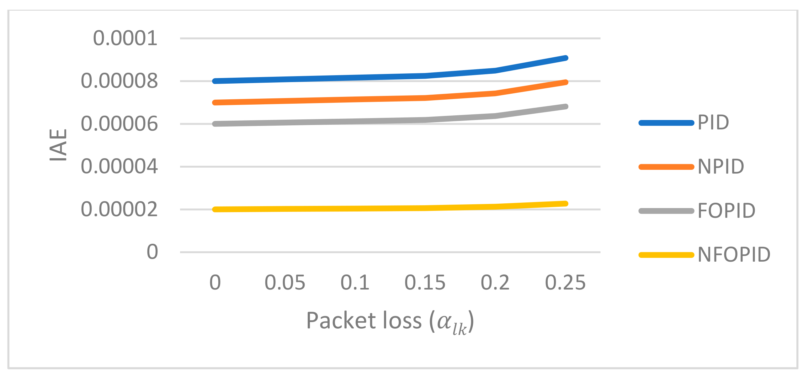
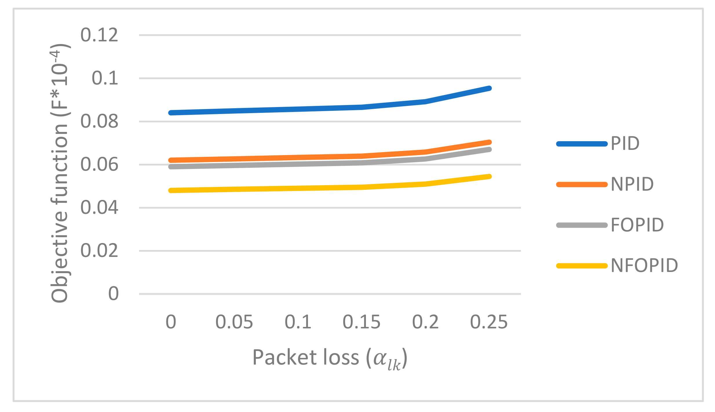
In this test, the delay time (ΓPC and ΓCA) is assumed to be constant and equals 40 milli-seconds. The packet loss () is assumed to range between [0, 0.25]. The change of the objective function, ITAE and IAE with respect to the change in packet loss values are shown in Figure 15, Figure 16 and Figure 17, respectively. The results show that NFOPID drives the system to better responses than the other control schemes.
8. Discussion
The paper presents an idea towards performing 100% renewable energy associated with organic agriculture farms in Africa. The paper assumed the presence of interconnection between two farms microgrids feeding from bioenergy and solar energy technologies only in the presence of battery and flywheel storage systems. A new optimization technique is used to tune the parameters of the controllers to get optimal frequency performance at different operating conditions considering 5G communication delays. Three modern control schemes are proposed, i.e., NFOPID, FOPID, and NPID, to control the interconnected microgrids. Five tests are performed to monitor the change in frequencies, tie-line power and generated powers at different operation conditions.
Test 1 shows that PRO algorithm is better than state of the art algorithms (SELO, PSO and GOZ) in terms of ITAE, IAE and objective function. The ITAE of PRO is less than SELO, GOZ, and PSO by 10.5%, 19%, and 34% respectively. The IAE of PRO is less than SELO, GOZ, and PSO by 31.25%, 42%, and 57.7% respectively. Test 1 also proved that, in the morning when a sudden load increase occurs, the bioenergy contributes to cover the increase in consumption.
Test 2 shows that the NFOPID control scheme is better than other proposed control schemes (FOPID, NPID, and PID control schemes) in terms of ITAE, IAE, and objective function. The ITAE of NFOPID is less than FOPID, NPID, and PID by 34.4%, 42%, and 56.3%, respectively. The IAE of NFOPID is less than FOPID, NPID, and PID by 11%, 14%, and 21%, respectively. Test 2 also proved that, at night when a sudden load increase occurs, the bioenergy contributes to cover the increase in consumption.
Test 3 shows that NFOPID control scheme is better than other proposed control schemes (FOPID, NPID, and PID control schemes) in terms of ITAE, IAE and objective function at SEKEM farm in Egypt (real case study). The ITAE of NFOPID is less than FOPID, NPID, and PID by 54.3%, 57% and 63% respectively. The IAE of NFOPID is less than FOPID, NPID, and PID by 67%, 71%, and 82%, respectively. Test 3 also proved that at SEKEM farm average daily real demand consumption and solar radiation, the bioenergy contributes to cover the change in demand consumption and solar radiation.
Test 4 shows that NFOPID control scheme is better than other proposed control schemes (FOPID, NPID, and PID control schemes) in terms of ITAE, IAE, and objective function at different 5G delay time from sensors to controllers and from controllers to actuators. The ITAE of NFOPID at 100 msec delay is less than FOPID, NPID, and PID by 37%, 41%, and 66% respectively. The IAE of NFOPID at 100 msec delay is less than FOPID, NPID, and PID by 13%, 17%, and 24%, respectively. Test 4 also proved that NFOPID drives the system to minimize the effect of time delay on the microgrids frequencies and powers.
Test 5 shows that NFOPID control scheme is better than other proposed control schemes (FOPID, NPID, and PID control schemes) in terms of ITAE, IAE, and objective function at different 5G packet loss. The ITAE of NFOPID at 0.25 packet loss is less than FOPID, NPID, and PID by 61%, 67%, and 81% respectively. The IAE of NFOPID at 0.25 packet loss is less than FOPID, NPID, and PID by 8%, 10%, and 14%, respectively. Test 5 also proved that NFOPID drives the system to minimize the effect of packet loss on the microgrids frequencies and powers.
9. Conclusions
The paper presented a two-area microgrid feeding from solar energy and bioenergy technologies with only information data transferred through 5G. The paper is a good step towards achieving energy food nexus and sustainable development goals in Africa. The research results show that the biogas and biodiesel generating systems contribute faster than the storage facilities to the change of demand and solar power. The paper presented a novel optimization technique PRO which demonstrated greater effectiveness than state of the art techniques in terms of a smaller number of iterations, IAE, ITAE, frequencies, and tie-line transient responses. The paper also presented a comparison between four different types of controllers on the system, which are NFOPID, PID, FOPID, and NPID. The results show that NFOPID drives the system to better performance than the other three controllers in terms of minimum ITAE, IAE, maximum overshoot, settling time, and maximum undershoot. The results also proved that FOPID has better performance than NPID. The conventional PID comes in the fourth place after the NPID. The results show the effect of time delay and packet loss on the system performance using each control scheme. The results proved that NFOPID will drive the system to better performance than the rest of the control schemes in terms of ITAE, IAE, and objective function.
Funding
This research received no external funding.
Conflicts of Interest
The authors declare no conflict of interest.
References
- Fayek, H.H. Load Frequency Control of a Power System with 100% Renewables. In Proceedings of the 2019 54th International Universities Power Engineering Conference (UPEC), Bucharest, Romania, 3–6 September 2019; pp. 1–6. [Google Scholar] [CrossRef]
- Das, D.C.; Sinha, N.; Roy, A.K. Automatic generation control of an organic rankine cycle solar–thermal/wind–diesel hybrid energy system. Energy Technol. 2014, 2, 721–731K. [Google Scholar] [CrossRef]
- Kroposki, B.; Johnson, B.; Zhang, Y.; Gevorgian, V.; Denholm, P.; Hodge, B.M.; Hannegan, B. Achieving a 100% Renewable Grid: Operating Electric Power Systems with Extremely High Levels of Variable Renewable Energy. IEEE Power Energy Mag. 2017, 15, 61–73. [Google Scholar] [CrossRef]
- Abdalla, O.H.; Fayek, H.H.; Abdel Ghany, A.M. Secondary Voltage Control Application in a Smart Grid with 100% Renewables. Inventions 2020, 5, 37. [Google Scholar] [CrossRef]
- Denholm, P.; Margolis, R. Energy Storage Requirements for Achieving 50% Solar Photovoltaic Energy Penetration in California; NREL: Golden, CO, USA, 2016. [Google Scholar]
- Renewable Energy Policy Network for the 21st CENTURY Annual Report. 2017. Available online: http://www.ren21.net (accessed on 20 January 2020).
- Bai, C.; Sarkis, J. The Water, Energy, Food, and Sustainability Nexus Decision Environment: A Multistakeholder Transdisciplinary Approach. IEEE Trans. Eng. Manag. 2019. [Google Scholar] [CrossRef]
- Barik, A.K.; Das, D.C. Expeditious frequency control of solar photovoltaic/biogas/biodiesel generator based isolated renewable microgrid using grasshopper optimisation algorithm. IET Renew. Power Gener. 2018, 12, 1659–1667. [Google Scholar] [CrossRef]
- Rasul, M.G.; Ault, C.; Sajjad, M. Bio-gas mixed fuel micro gas turbine cogeneration for meeting power demand in Australian remote areas. Energy Proc. 2015, 75, 1065–1071. [Google Scholar] [CrossRef]
- Muthu, D.; Venkatasubramanian, C.; Ramakrishnan, K.; Sasidhar, J. Production of biogas from wastes blended with cowdung for electricity generation-a case study. IOP Conf. Ser. Earth Environ. Sci. 2017, 80, 012055. [Google Scholar] [CrossRef] [Green Version]
- Liguori, V. Numerical investigation: Performances of a standard biogas in a 100 kWe MGT. Energy Rep. 2016, 2, 99–106. [Google Scholar] [CrossRef] [Green Version]
- Nabi, M.N.; Akhter, M.S.; Shahadat, M.M.Z. Improvement of engine emissions with conventional diesel fuel and diesel–biodiesel blends. Bioresour. Technol. 2006, 97, 372–378. [Google Scholar] [CrossRef]
- Basha, S.A.; Gopal, K.R.; Jebaraj, S. A review on biodiesel production, combustion, emissions and performance. Renew. Sustain. Energy Rev. 2009, 13, 1628–1634. [Google Scholar] [CrossRef]
- Fayek, H.H.; El-Zoghby, H.; Abdel Ghany, A.M. Design of Robust PID Controllers Using H∞ Technique to Control the Frequency of Wind-Diesel-Hydro Hybrid Power System. In Proceedings of the 9th International Conference on Electrical Engineering (ICEENG 2014), Cairo, Egypt, 27–29 May 2014; pp. 1–18. [Google Scholar]
- Birs, I.; Muresan, C.; Nascu, I.; Ionescu, C. A Survey of Recent Advances in Fractional Order Control for Time Delay Systems. IEEE Access 2019, 7, 30951–30965. [Google Scholar] [CrossRef]
- Fayek, H.H.; Mohammadi-Ivatloo, B. Tidal Supplementary Control Schemes-Based Load Frequency Regulation of a Fully Sustainable Marine Microgrid. Inventions 2020, 5, 53. [Google Scholar] [CrossRef]
- Ghoshal, S.P. Optimizations of PID gains by particle swarm optimizations in fuzzy based automatic generation control. Electr. Power Syst. Res. 2004, 72, 203–212. [Google Scholar] [CrossRef]
- Saremi, S.; Mirjalili, S.A.; Lewis, A. Grasshopper Optimization Algorithm: Theory and application. Adv. Eng. Softw. 2017, 105, 30–47. [Google Scholar] [CrossRef]
- Kumar, M.; Kulkarni, A.J.; Satapathy, S.C. Socio evolution & learning optimization algorithm: A socio-inspired optimization methodology. Future Gener. Comput. Syst. 2018, 81, 252–272. [Google Scholar]
- Moosavi, S.H.; Bardsiri, V.K. Poor and rich optimization algorithm: A new human-based and multi populations algorithm. Eng. Appl. Artif. Intell. 2019, 86, 165–181. [Google Scholar] [CrossRef]
- Fan, J.; Jiang, Y.; Chai, T. MPC-based setpoint compensation with unreliable wireless communications and constrained operational conditions. Neurocomputing 2017, 270, 110–121. [Google Scholar] [CrossRef]
- Alfergani, A.; Khalil, A.; Rajab, Z. Networked control of AC microgrid. Sustain. Cities Soc. 2018, 37, 371–387. [Google Scholar] [CrossRef]
- Mo, H.; Sansavini, G. Real-time coordination of distributed energy resources for frequency control in microgrids with unreliable communication. Int. J. Electr. Power Energy Syst. 2018, 96, 86–105. [Google Scholar] [CrossRef]
- Batista, N.C.; Melício, R.; Matias, J.C.O.; Catalão, J.P.S. Photovoltaic and wind energy systems monitoring and building/home energy management using ZigBee devices within a smart grid. Energy 2013, 49, 306–315. [Google Scholar] [CrossRef]
- Eissa, M.M. New protection principle for smart grid with renewable energy sources integration using WiMAX centralized scheduling technology. Int. J. Electr. Power Energy Syst. 2018, 97, 372–384. [Google Scholar]
- Siow, L.K.; So, P.L.; Gooi, H.B.; Luo, F.L.; Gajanayake, C.J.; Vo, Q.N. Wi-Fi based server in microgrid energy management system. In Proceedings of the IEEE Region 10 Conference 2009, Singapore, 23–26 January 2009; pp. 1–5. [Google Scholar]
- Rana, M.; Li, L.; Su, S. Kalman filter based microgrid state estimation and control using the IoT with 5G networks. In Proceedings of the IEEE PES Asia–Pacific Power Energy Engineering Conference (APPEEC), Brisbane, Australia, 15–18 November 2015; pp. 1–5. [Google Scholar]
- RES4AFRICA Website. Available online: https://www.res4africa.org/water-energy-food-nexus/ (accessed on 2 February 2020).
- Shah, P.; Agashe, S. Review of fractional PID controller. Mechatronics 2016, 38, 29–41. [Google Scholar] [CrossRef]
- Ausloos, M.; Dirickx, M. The Logistic Map and the Route to Chaos; Springer: Berlin, Germany, 2006. [Google Scholar]
- Oustaloup, A.; Levron, F.; Mathieu, B.; Nanot, F.M. Frequency-band complex noninteger differentiator: Characterization and synthesis. IEEE Trans. Circuits Syst. I Fundam. Theory Appl. 2000, 47, 25–39. [Google Scholar] [CrossRef]
- Micev, M.; Ćalasan, M.; Oliva, D. Fractional Order PID Controller Design for an AVR System Using Chaotic Yellow Saddle Goatfish Algorithm. Mathematics 2020, 8, 1182. [Google Scholar] [CrossRef]
- Fayek, H.H. Robust Controllers Design of Hybrid System Load Frequency Control. Master’s Thesis, Helwan University, Helwan, Egypt, 2014. [Google Scholar]
- Rashad, S.A.; Sallam, M.; Bassiuny, A.M.; Abdelghany, A.M. Control of Master-Slave System Using Optimal NPID and FOPID. In Proceedings of the 2019 IEEE 28th International Symposium on Industrial Electronics (ISIE), Vancouver, BC, Canada, 12–14 June 2019; pp. 485–490. [Google Scholar] [CrossRef]
- Pahadasingh, S.; Jena, C.; Panigrahi, C.K. Load frequency control incorporating electric vehicles using FOPID controller with HVDC link. In Innovation in Electrical Power Engineering, Communication, and Computing Technology; Sharma, R., Mishra, M., Nayak, J., Naik, B., Pelusi, D., Eds.; Lecture Notes in Electrical Engineering; Springer: Singapore, 2020; Volume 630. [Google Scholar] [CrossRef]
- Mehra, V.; Srivastava, S.; Varshney, P. Fractional-Order PID Controller Design for Speed Control of DC Motor. In Proceedings of the 2010 3rd International Conference on Emerging Trends in Engineering and Technology, Goa, India, 19–21 November 2010; pp. 422–425. [Google Scholar] [CrossRef]
- Jeba, P.; Selvakumar, A.I. FOPID based MPPT for photovoltaic system. Energy Sources Part A Recovery Util. Environ. Eff. 2018, 40, 1591–1603. [Google Scholar] [CrossRef]
- Wang, Z.; Wang, X.; Liu, L. Stochastic optimal linear control of wireless networked control systems with delays and packet losses. IET Control Theory Appl. 2016, 10, 742–751. [Google Scholar] [CrossRef] [Green Version]
- SEKEM Farm. Available online: https://www.sekem.com/en/index/ (accessed on 20 September 2020).
Figure 1.
Hybrid solar energy and bioenergy idea and system.

Figure 2.
Hybrid system SIMULINK model.

Figure 3.
NFOPID controller modes of operation.

Figure 4.
NFOPID controller configuration.

Figure 5.
PRO optimization flow chart.
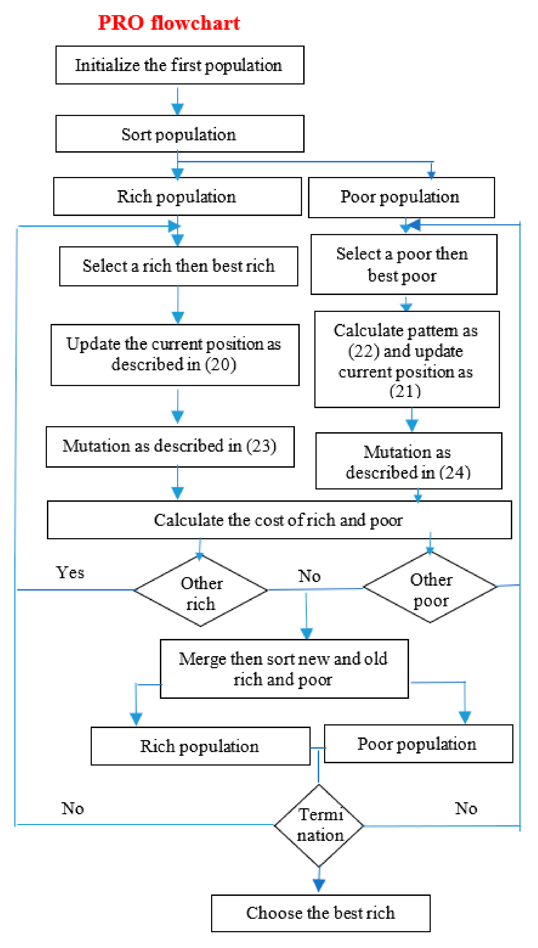
Figure 6.
System monitoring and communication.
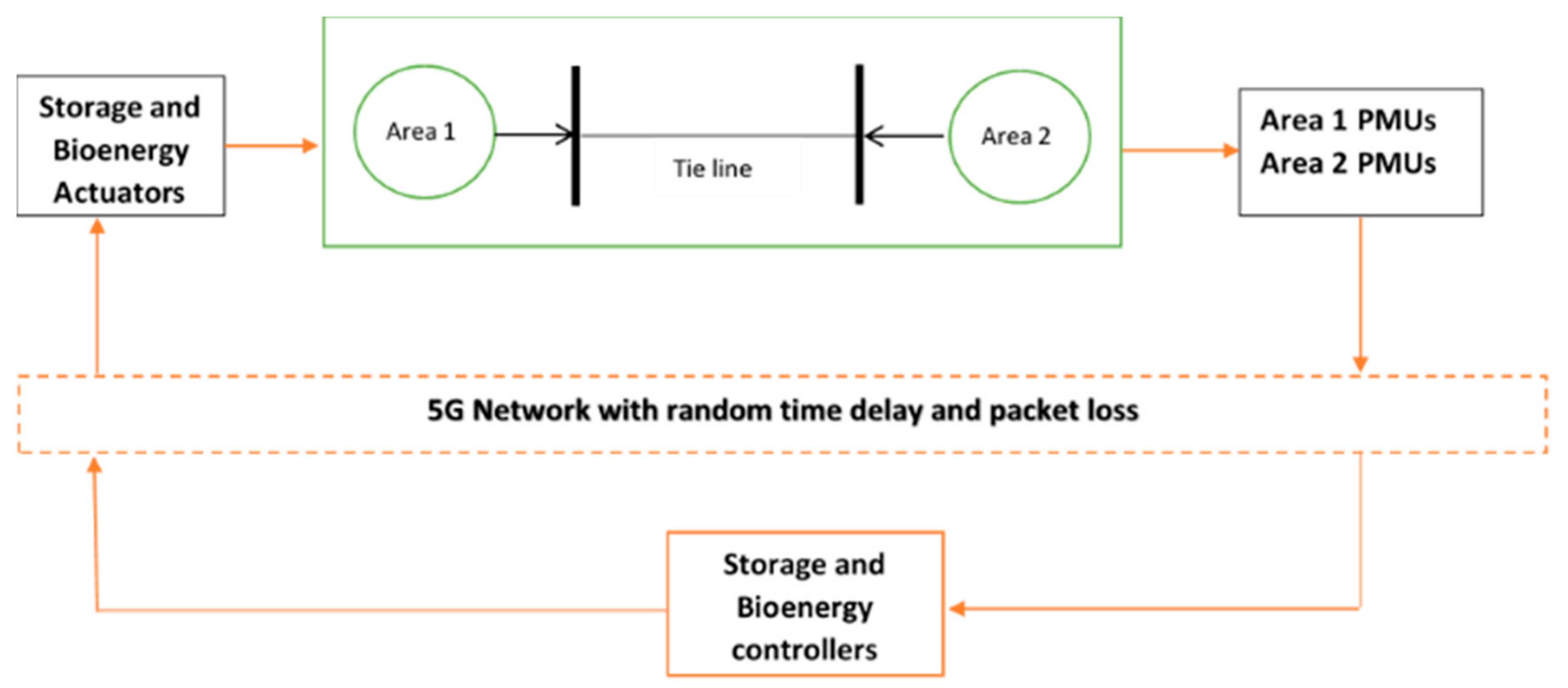
Figure 7.
Change in areas 1 and 2 frequencies in addition to change in tie line power at Test 1.

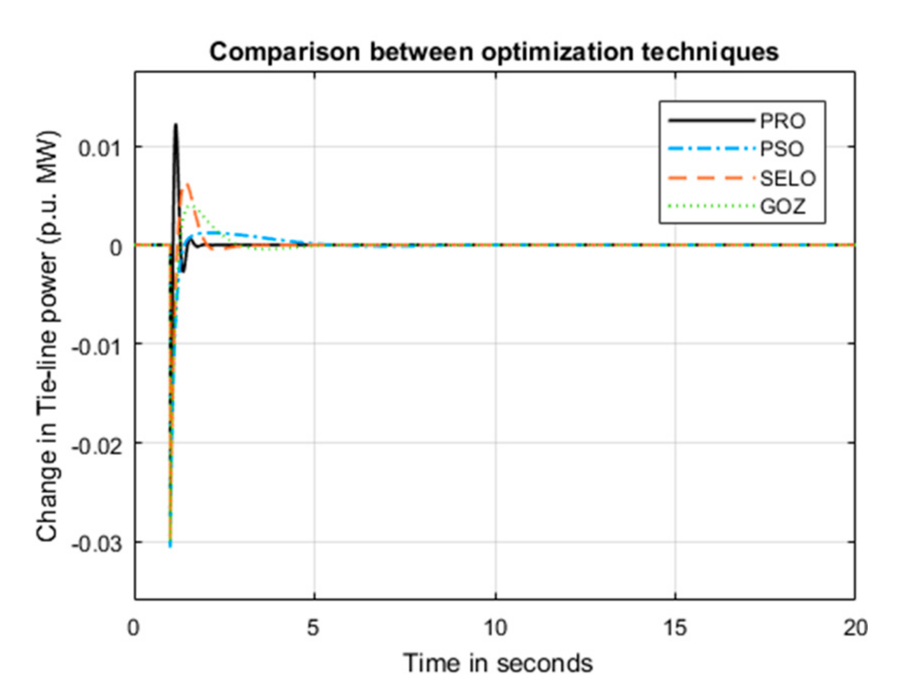
Figure 8.
Change in areas 1 and 2 bioenergy and storage generation at Test 1.
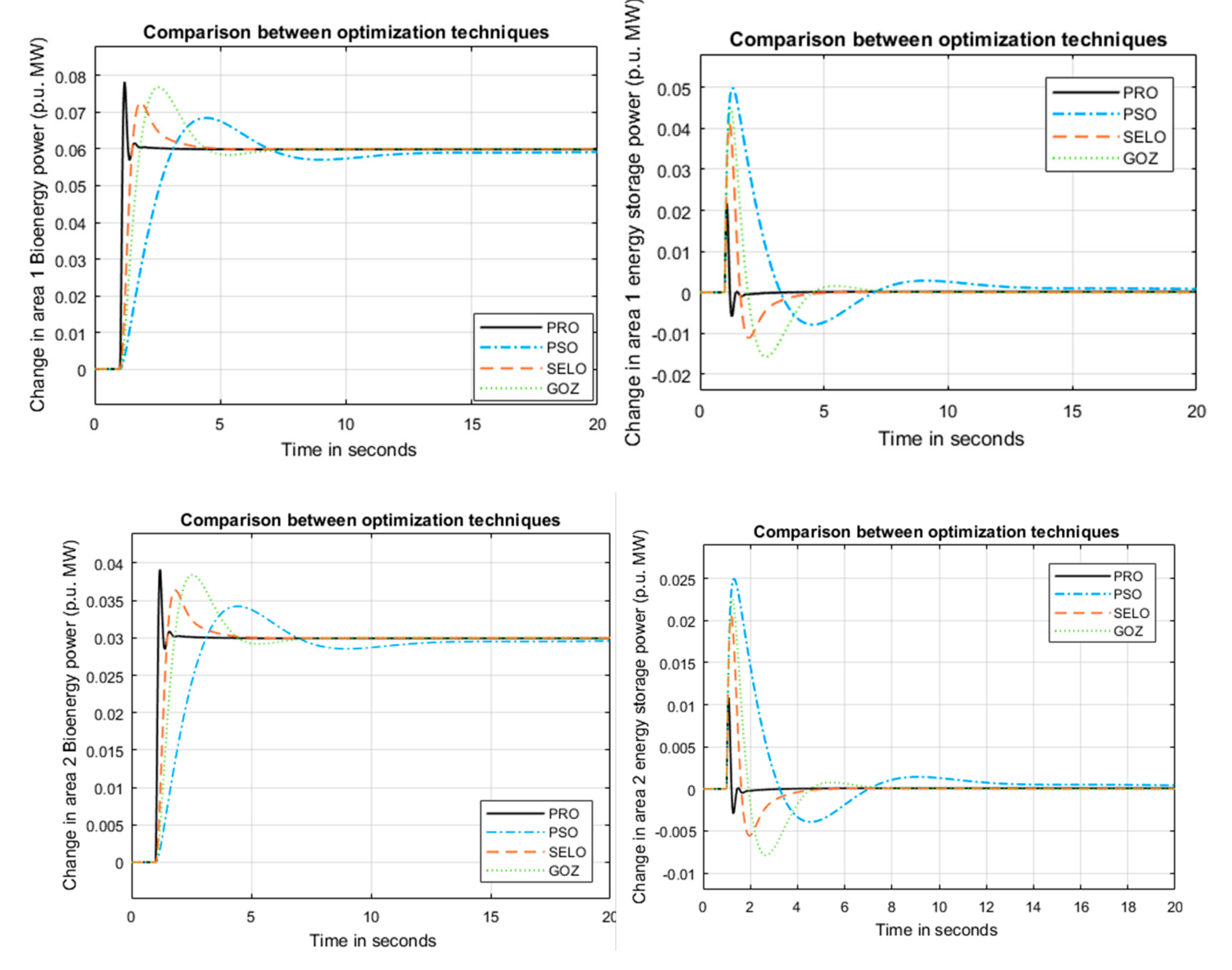
Figure 9.
Change in areas 1 and 2 frequencies in addition to change in tie line power at Test 2.
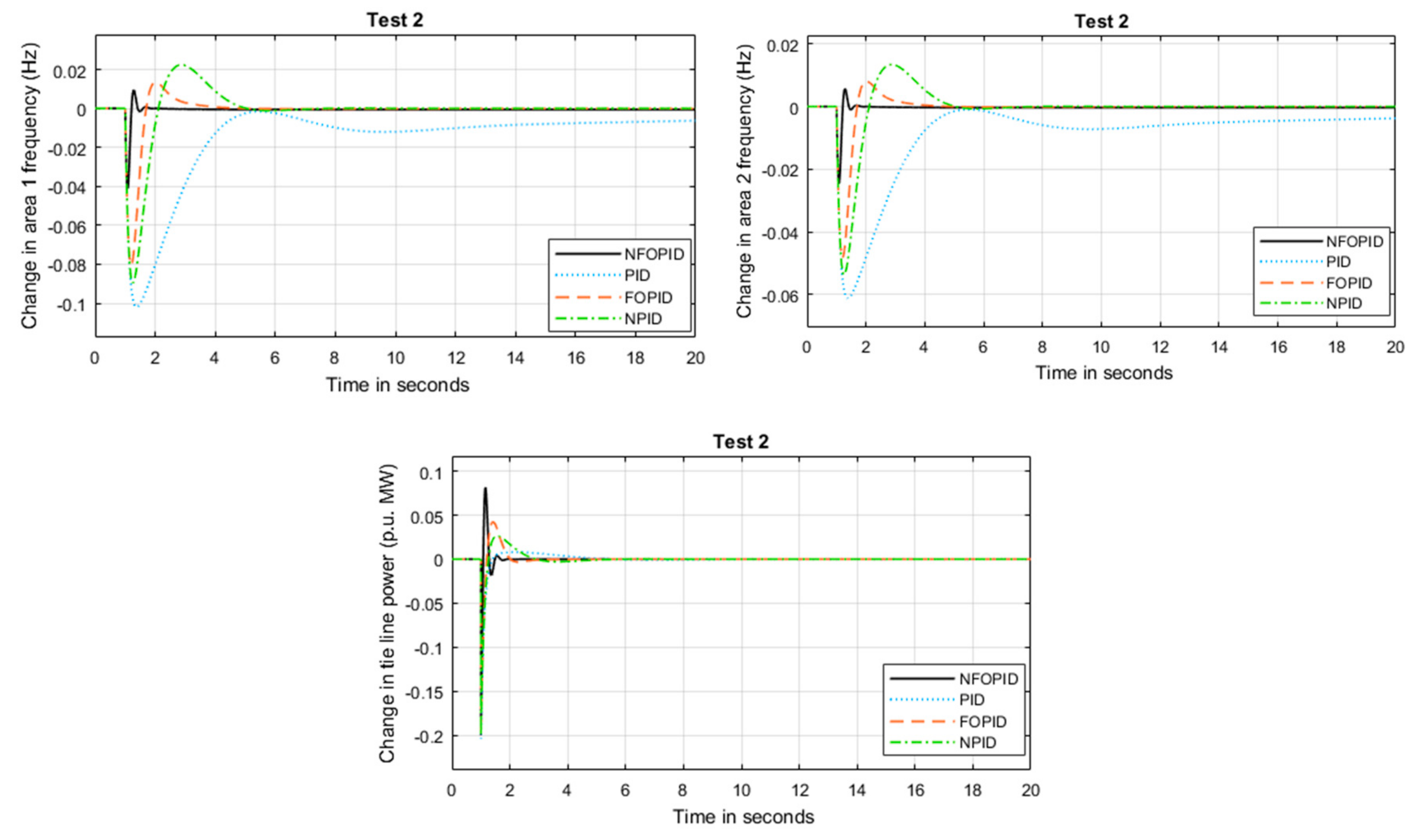
Figure 10.
Change in areas 1 and 2 bioenergy and storage generation at Test 2.
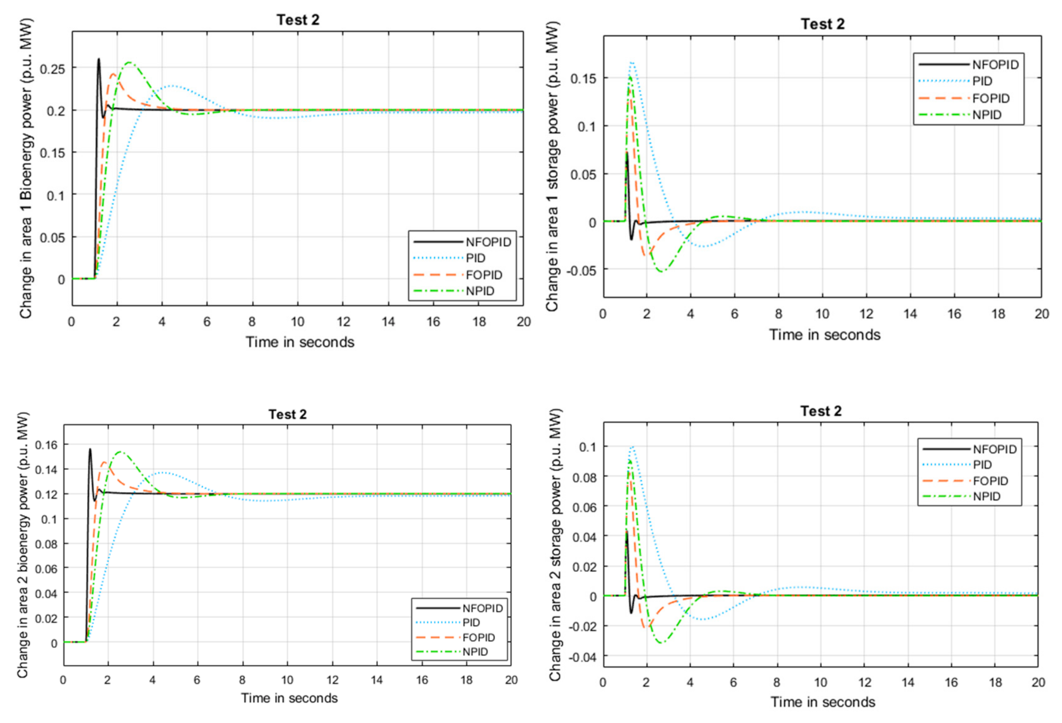
Figure 11.
Change in frequency, generated power, and demand power at Test 3.
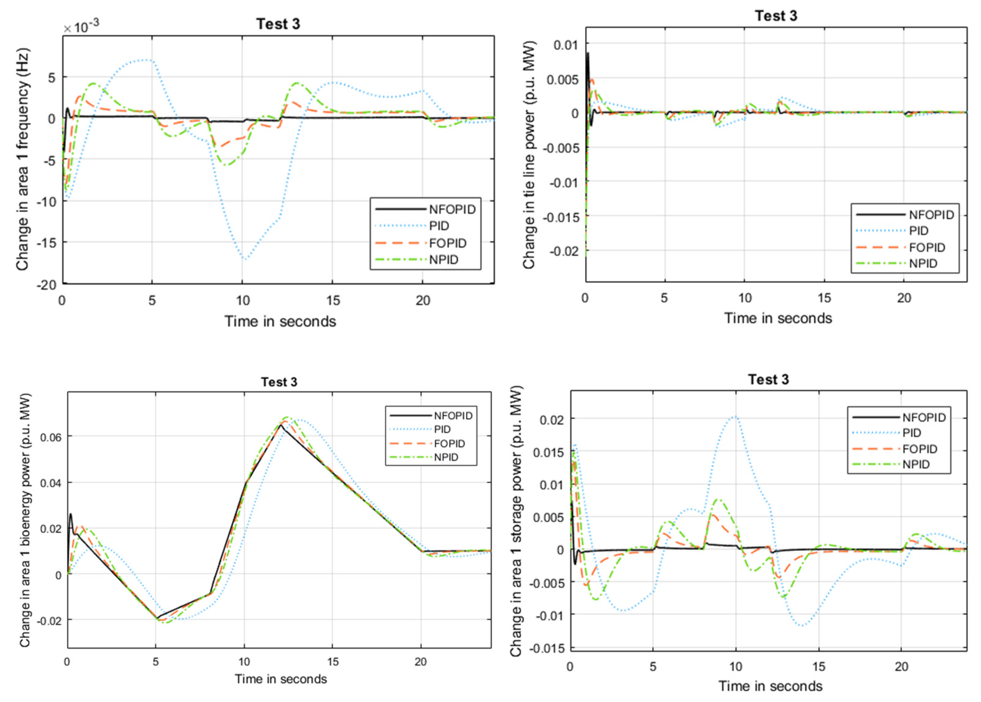
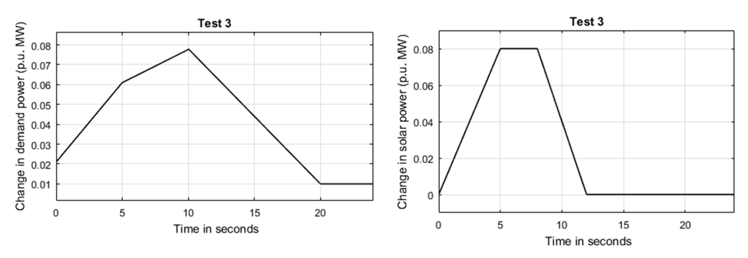
Figure 12.
Objective function at different delay time values for each control scheme.

Figure 13.
ITAE at different delay time values for each control scheme.
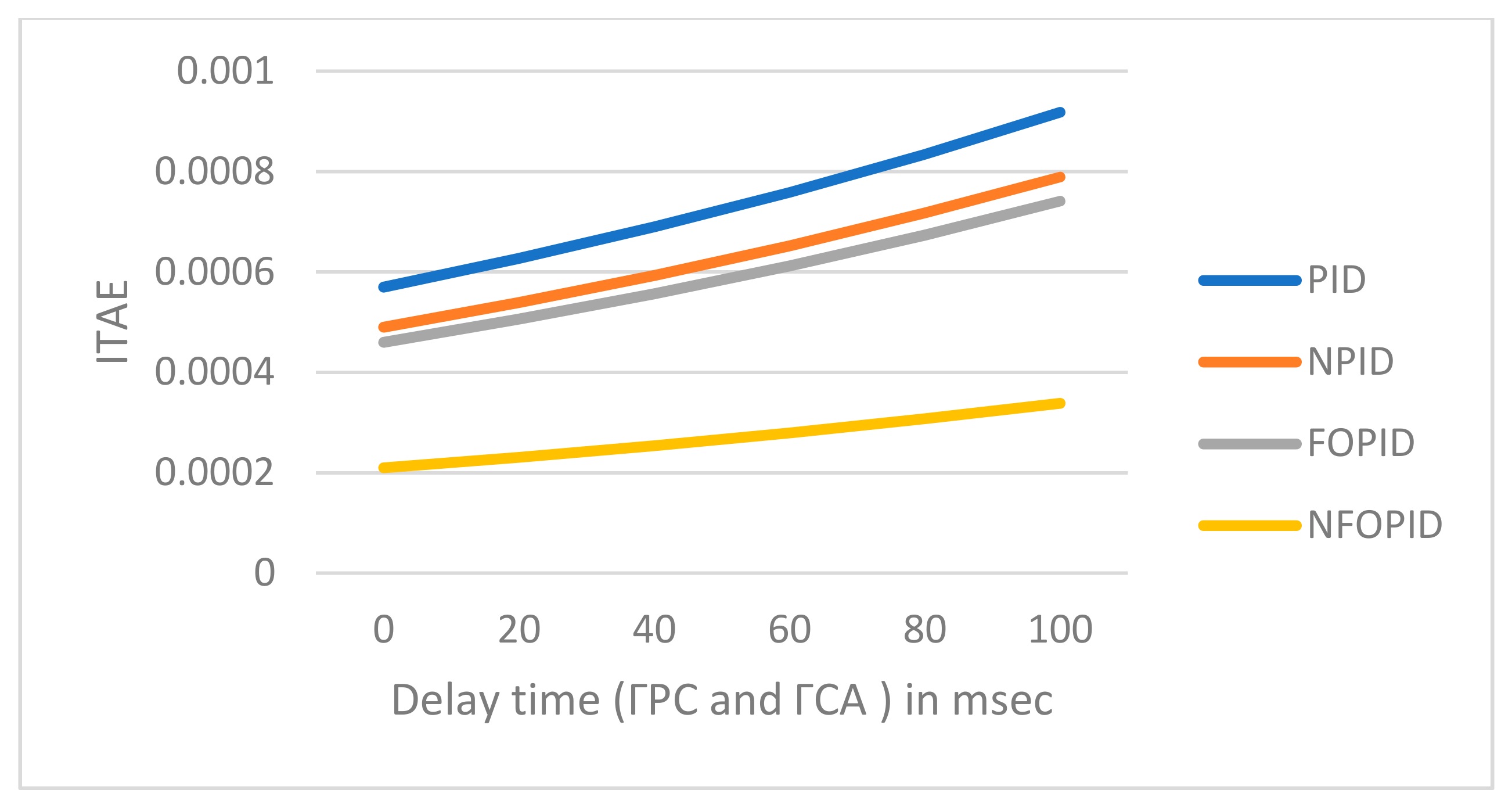
Figure 14.
IAE at different delay time values for each control scheme.

Figure 15.
Objective function at different Packet loss values for each control scheme.

Figure 16.
ITAE at different Packet loss values for each control scheme.

Figure 17.
IAE at different Packet loss values for each control scheme.

| Parameter | Value |
|---|---|
| 1.8 s | |
| 1 | |
| 0.3 s | |
| 1.8 | |
| 1.8 s | |
| 0.01 | |
| 0.23 s | |
| 0.6 s | |
| 1 | |
| 0.05 | |
| 0.2 s | |
| 1 | |
| 0.05s | |
| 1 | |
| 0.5 s | |
| 0.0033 | |
| 0.1 s | |
| 0.01 | |
| 0.1 s | |
| 0.2 s | |
| D | 0.012 |
| B | 18.4 |
| T12 | 1.9 |
| 0.5 | |
| 0.5 |
Table 2.
Comparison between optimization methods at Test 1.
| Method | ITAE | IAE | F × 10−4 | Number of Iterations | Transient Response of | Transient Response of | Transient Response of ΔPtie | ||||||
|---|---|---|---|---|---|---|---|---|---|---|---|---|---|
| Ush × 10−3 | Osh × 10−3 | ts | Ush × 10−3 | Osh × 10−3 | ts | Ush × 10−3 | Osh × 10−3 | ts | |||||
| PRO | 0.017 | 0.0033 | 0.39 | 15 | −11 | 2.5 | 2 | −5 | 1 | 2 | −20 | 11 | 2 |
| SELO | 0.019 | 0.0048 | 0.42 | 21 | −24 | 4 | 4 | −11 | 1.5 | 4 | −30 | 6 | 4 |
| GOZ | 0.021 | 0.0057 | 0.48 | 18 | −26 | 7 | 5 | −13 | 2.5 | 5 | −30 | 5 | 5 |
| PSO | 0.026 | 0.0078 | 0.61 | 25 | −30 | 0 | 20 | −15 | 0 | 20 | −30 | 2 | 12 |
Table 3.
Comparison between control schemes at Test 2.
| Control Scheme | ITAE | IAE | F × 10−4 | Transient Response of | Transient Response of | Transient Response of ΔPtie | ||||||
|---|---|---|---|---|---|---|---|---|---|---|---|---|
| Ush × 10−3 | Osh × 10−3 | ts | Ush × 10−3 | Osh × 10−3 | ts | Ush × 10−3 | Osh × 10−3 | ts | ||||
| NFOPID | 0.021 | 0.0049 | 0.48 | −40 | 10 | 1.8 | −22 | 5 | 1.8 | −180 | 70 | 1.8 |
| FOPID | 0.032 | 0.0055 | 0.53 | −80 | 15 | 3.7 | −51 | 8 | 3.7 | −200 | 40 | 2.7 |
| NPID | 0.036 | 0.0057 | 0.56 | −85 | 22 | 4.7 | −55 | 12 | 4.7 | −200 | 25 | 3.5 |
| PID | 0.048 | 0.0062 | 0.67 | −100 | 0 | 20 | −60 | 0 | 20 | −200 | 15 | 4 |
Table 4.
Comparison between control schemes at Test 3.
| Controller | ITAE | IAE | F × 10−4 |
|---|---|---|---|
| PID | 0.00057 | 0.00008 | 0.084 |
| NPID | 0.00049 | 0.00007 | 0.062 |
| FOPID | 0.00046 | 0.00006 | 0.059 |
| NFOPID | 0.00021 | 0.00002 | 0.048 |
Publisher’s Note: MDPI stays neutral with regard to jurisdictional claims in published maps and institutional affiliations. |
© 2020 by the author. Licensee MDPI, Basel, Switzerland. This article is an open access article distributed under the terms and conditions of the Creative Commons Attribution (CC BY) license (http://creativecommons.org/licenses/by/4.0/).
Share and Cite
MDPI and ACS Style
Fayek, H.H. 5G Poor and Rich Novel Control Scheme Based Load Frequency Regulation of a Two-Area System with 100% Renewables in Africa. Fractal Fract. 2021, 5, 2. https://0-doi-org.brum.beds.ac.uk/10.3390/fractalfract5010002
AMA Style
Fayek HH. 5G Poor and Rich Novel Control Scheme Based Load Frequency Regulation of a Two-Area System with 100% Renewables in Africa. Fractal and Fractional. 2021; 5(1):2. https://0-doi-org.brum.beds.ac.uk/10.3390/fractalfract5010002
Chicago/Turabian StyleFayek, Hady H. 2021. "5G Poor and Rich Novel Control Scheme Based Load Frequency Regulation of a Two-Area System with 100% Renewables in Africa" Fractal and Fractional 5, no. 1: 2. https://0-doi-org.brum.beds.ac.uk/10.3390/fractalfract5010002