A Generalization of a Fractional Variational Problem with Dependence on the Boundaries and a Real Parameter

Abstract

In this paper, we present a new fractional variational problem where the Lagrangian depends not only on the independent variable, an unknown function and its left- and right-sided Caputo fractional derivatives with respect to another function, but also on the endpoint conditions and a free parameter. The main results of this paper are necessary and sufficient optimality conditions for variational problems with or without isoperimetric and holonomic restrictions. Our results not only provide a generalization to previous results but also give new contributions in fractional variational calculus. Finally, we present some examples to illustrate our results.

1. Introduction

Non-integer calculus, known as fractional calculus, deals with integrals and derivatives with arbitrary real or complex orders [1,2]. It has developed in the past decades, becoming an important tool in applied sciences and engineering. Nowadays, fractional calculus is an important subject, e.g., in physics [3,4], robot trajectory controllers [5], heat diffusion [6], signal and image processing [7], or biology [8,9].

A question that arises when dealing with fractional calculus is which fractional integral or derivative should we choose? There are several definitions proposed, such as Riemann–Liouville, Caputo, Hadamard, Erdélyi–Kober, Grünwald–Letnikov, Weyl, or Marchaud fractional operators. However, there are ways to overcome this issue, considering a more general class of operators. In [2], we find the concept of fractional derivative with respect to another function. For particular choices of such function, we obtain some of the previous ones. We denote the fractional order by $\alpha \in {\mathbb{R}}^{+}$, and let $\psi \in C^1([a,b],\mathbb{R})$ be a function with ${\psi }^{\prime }\left(t\right)>0$, for all $t\in [a,b]$. Given an integrable function $x:[a,b]\to \mathbb{R}$, the left-sided and the right-sided Riemann–Liouville fractional integrals of x with kernel $\psi$ are defined as

$$\left(I_{a^{+}}^{\alpha ,\psi }x\right)\left(t\right):=\frac{1}{\Gamma \left(\alpha \right)}{\int }_a^t{\psi }^{\prime }\left(\tau \right){(\psi \left(t\right)-\psi \left(\tau \right))}^{\alpha -1}x\left(\tau \right)d\tau ,t>a,$$

and

$$\left(I_{b^{-}}^{\alpha ,\psi }x\right)\left(t\right):=\frac{1}{\Gamma \left(\alpha \right)}{\int }_t^b{\psi }^{\prime }\left(\tau \right){(\psi \left(\tau \right)-\psi \left(t\right))}^{\alpha -1}x\left(\tau \right)d\tau ,t<b,$$

respectively, where $\Gamma$ represents the Gamma function, and $\alpha$ is the order of the fractional integral. Moreover,

$$I_{a^{+}}^{\alpha ,\psi }x=I_{b^{-}}^{\alpha ,\psi }x=x,as\alpha \to 0^{+}.$$

We can recognize that the Riemann–Liouville, the Hadamard and the Erdélyi–Kober fractional integrals are just particular cases of this more general definition. With respect to fractional differentiation, the left- and right-sided Riemann–Liouville fractional derivatives of x, with kernel $\psi$, are given by the formulas

$$\left(D_{a^{+}}^{\alpha ,\psi }x\right)\left(t\right):={\left(\frac{1}{{\psi }^{\prime }\left(t\right)}\frac{d}{dt}\right)}^n\left(I_{a^{+}}^{n-\alpha ,\psi }x\right)\left(t\right),t>a,$$

and

$$\left(D_{b^{-}}^{\alpha ,\psi }x\right)\left(t\right):={\left(-\frac{1}{{\psi }^{\prime }\left(t\right)}\frac{d}{dt}\right)}^n\left(I_{b^{-}}^{n-\alpha ,\psi }x\right)\left(t\right),t<b,$$

where $n=\left[\alpha \right]+1$. For simplicity, we call the last operators as $\psi$-Riemann–Liouville fractional derivatives of x of order $\alpha$. It can be easily noticed that for certain choices of function $\psi$, we recover some important fractional derivatives. We also remark that when $\alpha =m\in \mathbb{N}$, we have

$$\left(D_{a^{+}}^{\alpha ,\psi }x\right)\left(t\right)={\left(\frac{1}{{\psi }^{\prime }\left(t\right)}\frac{d}{dt}\right)}^{m}x\left(t\right)and\left(D_{b^{-}}^{\alpha ,\psi }x\right)\left(t\right)={\left(-\frac{1}{{\psi }^{\prime }\left(t\right)}\frac{d}{dt}\right)}^{m}x\left(t\right).$$

It is worth mentioning that, opposite to the ordinary derivatives, fractional derivatives are non-local and, in the case of left-sided derivatives, take into account the past. This is particularly useful for problems in different areas, such as economics, epidemiology, and optimal control problems [10,11,12,13].

Recently, in [14], motivated by the concept of Caputo fractional derivative and by these generalized fractional operators, the following definition was presented. Let $\alpha >0$ and $n\in \mathbb{N}$ be defined by $n=\left[\alpha \right]+1$ if $\alpha \notin \mathbb{N}$, and $n=\alpha$ if $\alpha \in \mathbb{N}$. Given two functions $x,\psi \in C^n([a,b],\mathbb{R})$, with ${\psi }^{\prime }\left(t\right)>0$, for all $t\in [a,b]$, the left- and right-sided Caputo fractional derivatives of x with kernel $\psi$ (or simply, $\psi$-Caputo fractional derivatives of x), are defined as

$$\left({}^C{D}_{a^{+}}^{\alpha ,\psi }x\right)\left(t\right):=\left(I_{a^{+}}^{n-\alpha ,\psi }{\left(\frac{1}{{\psi }^{\prime }\left(t\right)}\frac{d}{dt}\right)}^{n}x\right)\left(t\right),t>a,$$

and

$$\left({}^C{D}_{b^{-}}^{\alpha ,\psi }x\right)\left(t\right):=\left(I_{b^{-}}^{n-\alpha ,\psi }{\left(-\frac{1}{{\psi }^{\prime }\left(t\right)}\frac{d}{dt}\right)}^{n}x\right)\left(t\right),t<b,$$

respectively. Thus, if $\alpha =m\in \mathbb{N}$, then

$$\left({}^C{D}_{a^{+}}^{\alpha ,\psi }x\right)\left(t\right)={\left(\frac{1}{{\psi }^{\prime }\left(t\right)}\frac{d}{dt}\right)}^{m}x\left(t\right)and\left({}^C{D}_{b^{-}}^{\alpha ,\psi }x\right)\left(t\right)={\left(-\frac{1}{{\psi }^{\prime }\left(t\right)}\frac{d}{dt}\right)}^{m}x\left(t\right).$$

For $\alpha \in {\mathbb{R}}^{+}\backslash \mathbb{N}$, then

$$\left({}^C{D}_{a^{+}}^{\alpha ,\psi }x\right)\left(t\right)=\frac{1}{\Gamma (n-\alpha )}{\int }_a^t{\psi }^{\prime }\left(\tau \right){(\psi \left(t\right)-\psi \left(\tau \right))}^{n-\alpha -1}{\left(\frac{1}{{\psi }^{\prime }\left(\tau \right)}\frac{d}{d\tau }\right)}^{n}x\left(\tau \right)d\tau$$

and

$$\left({}^C{D}_{b^{-}}^{\alpha ,\psi }x\right)\left(t\right)=\frac{1}{\Gamma (n-\alpha )}{\int }_t^b{\psi }^{\prime }\left(\tau \right){(\psi \left(\tau \right)-\psi \left(t\right))}^{n-\alpha -1}{\left(-\frac{1}{{\psi }^{\prime }\left(\tau \right)}\frac{d}{d\tau }\right)}^{n}x\left(\tau \right)d\tau .$$

We now present the following formulas (see Lemma 1 in [14]) that are useful in Section 3. If $n<\beta \in \mathbb{R}$, then

$${}^C{D}_{a^{+}}^{\alpha ,\psi }{(\psi \left(t\right)-\psi \left(a\right))}^{\beta -1}=\frac{\Gamma \left(\beta \right)}{\Gamma (\beta -\alpha )}{(\psi \left(t\right)-\psi \left(a\right))}^{\beta -\alpha -1}$$

and

$${}^C{D}_{b^{-}}^{\alpha ,\psi }{(\psi \left(b\right)-\psi \left(t\right))}^{\beta -1}=\frac{\Gamma \left(\beta \right)}{\Gamma (\beta -\alpha )}{(\psi \left(b\right)-\psi \left(t\right))}^{\beta -\alpha -1}.$$

Next, we present the following fractional integration by parts formulas that are fundamental for the proofs of our results. For a more detailed study of the $\psi$-Caputo fractional derivatives, we refer to [14].

Theorem 1.

[14] Let $x\in C\left(\right[a,b],\mathbb{R})$ and $y,\psi \in C^n([a,b],\mathbb{R})$ be two functions. Then,

$$\begin{array}{cc}\hfill {\int }_a^b& x\left(t\right)·\left({}^C{D}_{a^{+}}^{\alpha ,\psi }y\right)\left(t\right)dt={\int }_a^{b}y\left(t\right)·\left(D_{b^{-}}^{\alpha ,\psi }\frac{x}{{\psi }^{\prime }}\right)\left(t\right){\psi }^{\prime }\left(t\right)dt\hfill \\ \hfill & +{\left[\sum _{k=0}^{n-1}{\left(-\frac{1}{{\psi }^{\prime }\left(t\right)}\frac{d}{dt}\right)}^k\left(I_{b^{-}}^{n-\alpha ,\psi }\frac{x}{{\psi }^{\prime }}\right)\left(t\right)·{\left(\frac{1}{{\psi }^{\prime }\left(t\right)}\frac{d}{dt}\right)}^{n-k-1}y\left(t\right)\right]}_{t=a}^{t=b}\hfill \end{array}$$

and

$$\begin{array}{cc}\hfill {\int }_a^b& x\left(t\right)·\left({}^C{D}_{b^{-}}^{\alpha ,\psi }y\right)\left(t\right)dt={\int }_a^{b}y\left(t\right)·\left(D_{a^{+}}^{\alpha ,\psi }\frac{x}{{\psi }^{\prime }}\right)\left(t\right){\psi }^{\prime }\left(t\right)dt\hfill \\ \hfill & +{\left[\sum _{k=0}^{n-1}{(-1)}^{n-k}{\left(\frac{1}{{\psi }^{\prime }\left(t\right)}\frac{d}{dt}\right)}^k\left(I_{a^{+}}^{n-\alpha ,\psi }\frac{x}{{\psi }^{\prime }}\right)\left(t\right)·{\left(\frac{1}{{\psi }^{\prime }\left(t\right)}\frac{d}{dt}\right)}^{n-k-1}y\left(t\right)\right]}_{t=a}^{t=b}.\hfill \end{array}$$

In particular, when $0<\alpha <1$, Theorem 1 becomes

$${\int }_a^{b}x\left(t\right)·\left({}^C{D}_{a^{+}}^{\alpha ,\psi }y\right)\left(t\right)dt={\int }_a^{b}y\left(t\right)·\left(D_{b^{-}}^{\alpha ,\psi }\frac{x}{{\psi }^{\prime }}\right)\left(t\right){\psi }^{\prime }\left(t\right)dt+{\left[\left(I_{b^{-}}^{1-\alpha ,\psi }\frac{x}{{\psi }^{\prime }}\right)\left(t\right)·y\left(t\right)\right]}_{t=a}^{t=b}$$

and

$${\int }_a^{b}x\left(t\right)·\left({}^C{D}_{b^{-}}^{\alpha ,\psi }y\right)\left(t\right)dt={\int }_a^{b}y\left(t\right)·\left(D_{a^{+}}^{\alpha ,\psi }\frac{x}{{\psi }^{\prime }}\right)\left(t\right){\psi }^{\prime }\left(t\right)dt-{\left[\left(I_{a^{+}}^{1-\alpha ,\psi }\frac{x}{{\psi }^{\prime }}\right)\left(t\right)·y\left(t\right)\right]}_{t=a}^{t=b}.$$

Fractional calculus of variations started with the pioneering works of Riewe [15,16]. Since then, numerous works have appeared for different types of fractional derivatives and integrals. To mention a few in such vast literature, we can refer the reader to the books [17,18,19]. The goal is to extremize (minimize or maximize) a given functional, depending on some fractional operator. Due to the large number of fractional operators to choose from, we found several works dealing with similar subjects (e.g., [20,21,22,23,24,25,26]). By considering a more general form of fractional derivative, such as the one given in [14], we can study different problems in a general form. In [27], some calculus of variation problems were addressed, with dependence on this fractional derivative. Necessary and sufficient conditions of optimality were proven, such as the Euler–Lagrange equation, and the isoperimetric problem was studied, among others.

The main goal of this paper is to generalize the fractional variational problem studied in [27], considering the case where the Lagrangian depends not only on the independent variable, an unknown function and its left- and right-sided Caputo fractional derivatives with respect to another function, but also on the endpoints conditions and a free parameter. This type of generalized fractional variational problems cannot be solved using the classical theory. Our motivation for studying generalized variational problems where the Lagrangian explicitly depends on state values and a free parameter comes from interesting applications in economics [28] and in physics [29], respectively. It is worth mentioning that, since these types of fractional derivatives are generalizations of several fractional derivatives and our variational problem is a generalization of different types of fractional variational problems, many results available in the literature are corollaries of the results proven in this paper.

The organization of the paper is as follows. We start Section 2.1 considering the generalized fractional variational problem with fixed boundary conditions and proving a necessary optimality condition of Euler–Lagrange type and also a necessary condition which arises as a consequence of the Lagrangian dependence of the parameter. Then, we prove the natural boundary conditions for variational problems with free boundary conditions. In Section 2.2, we prove necessary optimality conditions for variational problems with integral constraints, with and without fixed boundary conditions. The variational problem with an holonomic constraint is studied in Section 2.3. In Section 2.4, we prove sufficient optimality conditions for the variational problems considered in the previous subsections. We conclude the paper with some illustrative examples and concluding remarks.

2. Main Results

In this work, we consider a functional depending on time, on the state function x, its fractional derivatives ${}^C{D}_{a^{+}}^{\alpha ,\psi }x$ and ${}^C{D}_{b^{-}}^{\beta ,\psi }x$ of orders $\alpha ,\beta \in ]0,1[$, the values $x\left(a\right)$ and $x\left(b\right)$, and a free parameter $\zeta$. More specifically, we will study the following generalized fractional variational problem.

Problem$\left(\mathcal{P}\right)$: Determine $x\in C^1([a,b],\mathbb{R})$ and $\zeta \in \mathbb{R}$ such that

$$\mathcal{J}(x,\zeta ):={\int }_a^{b}L[x,\zeta ]\left(t\right)dt⟶extremize$$

(1)

where $L\in C^1([a,b]\times {\mathbb{R}}^6,\mathbb{R})$ and

$$[x,\zeta ]\left(t\right):=\left(t,x\left(t\right),\left({}^C{D}_{a^{+}}^{\alpha ,\psi }x\right)\left(t\right),\left({}^C{D}_{b^{-}}^{\beta ,\psi }x\right)\left(t\right),x\left(a\right),x\left(b\right),\zeta \right).$$

We will consider problem $\left(\mathcal{P}\right)$ with fixed boundary conditions

$$x\left(a\right)=x_{a}andx\left(b\right)=x_b,$$

(2)

for some $x_a,x_b\in \mathbb{R}$, and when $x\left(a\right)$ and $x\left(b\right)$ are free. We will also consider problem $\left(\mathcal{P}\right)$ subject to an isoperimetric constraint

$$\mathcal{I}(x,\zeta ):={\int }_a^{b}F[x,\zeta ]\left(t\right)dt=\gamma ,$$

(3)

for some $\gamma \in \mathbb{R},$ and to an holonomic constraint

$$g(t,x(t),x(a),x(b),\zeta )=0,$$

for a given function g.

Remark 1.

We remark that:

• If the function $\psi =Id$, and the Lagrange function does not depend on a free parameter ζ, then we get the fractional variational problem studied in [30];
• Taking $\alpha \to 1^{-}$, and if ψ is the identity, the operators ${}^C{D}_{a^{+}}^{\alpha }$ and ${}^C{D}_{b^{-}}^{\alpha }$ can be replaced by $\frac{d}{dt}$ and $-\frac{d}{dt}$, respectively (see [1]). Hence, if α and β goes to 1, our functional $\mathcal{J}$ tends to the generalized variational functional ${\displaystyle {\int }_a^b\tilde{L}(t,x\left(t\right),x^{\prime }\left(t\right),x\left(a\right),x\left(b\right),\zeta )dt}$ of the classical calculus of variations studied in [31];
• If $\psi =Id$, α and β goes to 1, and the Lagrange function does not depend on the state values and on a free parameter, functional $\mathcal{J}$ reduces to the functional ${\displaystyle {\int }_a^{b}L(t,x\left(t\right),x^{\prime }\left(t\right))dt}$ from Lemma 2.2.2 in [32].

Next, we proceed with some basic definitions that are useful in what follows.

Definition 1.

Let $x\in C^1([a,b],\mathbb{R})$ and $\zeta \in \mathbb{R}$. We say that $(x,\zeta )$ is an admissible pair to $\left(\mathcal{P}\right)$ subject to (2), if x satisfies (2). Function $\eta \in C^1([a,b],\mathbb{R})$ is an admissible variation to $\left(\mathcal{P}\right)$ subject to (2) if $\eta \left(a\right)=\eta \left(b\right)=0$.

Definition 2.

We say that $(x^{🟉},{\zeta }^{🟉})$ is a local minimizer (resp. local maximizer) for the functional $\mathcal{J}$ if there exists some $\delta >0$, such that, for all $(x,\zeta )\in C^1([a,b],\mathbb{R})\times \mathbb{R}$ with $\parallel (x^{🟉},{\zeta }^{🟉})-(x,\zeta )\parallel <\delta$, we have $\mathcal{J}(x^{🟉},{\zeta }^{🟉})\le \mathcal{J}(x,\zeta )$ (resp. $\mathcal{J}(x^{🟉},{\zeta }^{🟉})\ge \mathcal{J}(x,\zeta )$), where $\parallel (x,\zeta )\parallel :={max}_{t\in [a,b]}\left|x\left(t\right)\right|+\left|\zeta \right|$. The pair $(x^{🟉},{\zeta }^{🟉})$ is called a local extremizer of $\mathcal{J}$.

If $\mathcal{J}(x^{🟉},{\zeta }^{🟉})\le \mathcal{J}(x,\zeta )$ (resp. $\mathcal{J}(x^{🟉},{\zeta }^{🟉})\ge \mathcal{J}(x,\zeta )$) holds for all $(x,\zeta )\in C^1([a,b],\mathbb{R})\times \mathbb{R}$, then we say that $(x^{🟉},{\zeta }^{🟉})$ is a global minimizer (resp. global maximizer). In these cases, we say that $(x^{🟉},{\zeta }^{🟉})$ is a global extremizer of $\mathcal{J}$.

2.1. Generalized Fractional Variational Principle

The following result provides necessary conditions for an admissible pair $(x,\zeta )$ to be a local extremizer of functional $\mathcal{J}$, where x satisfies the boundary conditions (2). The equation

$${\partial }_{2}L[x,\zeta ]\left(t\right)+\left(D_{b^{-}}^{\alpha ,\psi }\frac{{\partial }_{3}L[x,\zeta ]}{{\psi }^{\prime }}\right)\left(t\right){\psi }^{\prime }\left(t\right)+\left(D_{a^{+}}^{\beta ,\psi }\frac{{\partial }_{4}L[x,\zeta ]}{{\psi }^{\prime }}\right)\left(t\right){\psi }^{\prime }\left(t\right)=0,t\in [a,b],$$

(4)

is called the Euler–Lagrange equation. We will represent it by $ELe\left\{L\right[x,\zeta \left]\right\}$. To simplify, consider the two following conditions:

$$C^{+}[H,i]:t\mapsto \left(D_{a^{+}}^{\beta ,\psi }\frac{{\partial }_{i}H[x,\zeta ]}{{\psi }^{\prime }}\right)\left(t\right)\text{is continuous for all} t\in [a,b]$$

and

$$C^{-}[H,i]:t\mapsto \left(D_{b^{-}}^{\alpha ,\psi }\frac{{\partial }_{i}H[x,\zeta ]}{{\psi }^{\prime }}\right)\left(t\right)\text{is continuous for all} t\in [a,b],$$

where H is a function and i a positive integer.

Theorem 2

(Generalized fractional variational principle). Suppose that L satisfies $C^{+}[L,4]$ and $C^{-}[L,3]$. If $(x,\zeta )$ is a local extremizer of functional $\mathcal{J}$, subject to the boundary conditions (2), then Equation (4) holds. Additionally,

$${\displaystyle {\int }_a^b{\partial }_{7}L[x,\zeta ]\left(t\right)dt=0}$$

(5)

is verified.

Proof. 

Let $(x,\zeta )$ be a local extremizer for functional $\mathcal{J}$ subject to (2), $\eta$ an admissible variation and $\delta$ an arbitrary real number. Define the new function $\varphi :\mathbb{R}\to \mathbb{R}$ by $\varphi \left(ϵ\right)=\mathcal{J}(x+ϵ\eta ,\zeta +ϵ\delta )$. Since $(x,\zeta )$ is a local extremizer of $\mathcal{J}$, then ${\varphi }^{\prime }\left(0\right)=0$. Therefore, the following condition holds

$$\begin{array}{c}\hfill {\int }_a^b({\partial }_{2}L[x,\zeta ]\left(t\right)\eta \left(t\right)+{\partial }_{3}L[x,\zeta ]\left(t\right)\left({}^C{D}_{a^{+}}^{\alpha ,\psi }\eta \right)\left(t\right)+{\partial }_{4}L[x,\zeta ]\left(t\right)\left({}^C{D}_{b^{-}}^{\beta ,\psi }\eta \right)\left(t\right)\\ \hfill +{\partial }_{5}L[x,\zeta ]\left(t\right)\eta \left(a\right)+{\partial }_{6}L[x,\zeta ]\left(t\right)\eta \left(b\right)+{\partial }_{7}L[x,\zeta ]\left(t\right)\delta )dt=0.\end{array}$$

Using the fractional integration by parts formulas stated in Theorem 1, we get

$$\begin{array}{c}\hfill {\int }_a^b({\partial }_{2}L[x,\zeta ]\left(t\right)+\left(D_{b^{-}}^{\alpha ,\psi }\frac{{\partial }_{3}L[x,\zeta ]}{{\psi }^{\prime }}\right)\left(t\right){\psi }^{\prime }\left(t\right)+\left(D_{a^{+}}^{\beta ,\psi }\frac{{\partial }_{4}L[x,\zeta ]}{{\psi }^{\prime }}\right)\left(t\right){\psi }^{\prime }\left(t\right))·\eta \left(t\right)dt\\ \hfill +{\left[\left(I_{b^{-}}^{1-\alpha ,\psi }\frac{{\partial }_{3}L[x,\zeta ]}{{\psi }^{\prime }}\right)\left(t\right)·\eta \left(t\right)\right]}_{t=a}^{t=b}-{\left[\left(I_{a^{+}}^{1-\beta ,\psi }\frac{{\partial }_{4}L[x,\zeta ]}{{\psi }^{\prime }}\right)\left(t\right)·\eta \left(t\right)\right]}_{t=a}^{t=b}\\ \hfill +{\int }_a^b({\partial }_{5}L[x,\zeta ]\left(t\right)\eta \left(a\right)+{\partial }_{6}L[x,\zeta ]\left(t\right)\eta \left(b\right)+{\partial }_{7}L[x,\zeta ]\left(t\right)\delta )dt=0.\end{array}$$

(6)

Since $\eta \left(a\right)=\eta \left(b\right)=0$, then

$$\begin{array}{c}\hfill {\int }_a^b({\partial }_{2}L[x,\zeta ]\left(t\right)+\left(D_{b^{-}}^{\alpha ,\psi }\frac{{\partial }_{3}L[x,\zeta ]}{{\psi }^{\prime }}\right)\left(t\right){\psi }^{\prime }\left(t\right)+\left(D_{a^{+}}^{\beta ,\psi }\frac{{\partial }_{4}L[x,\zeta ]}{{\psi }^{\prime }}\right)\left(t\right){\psi }^{\prime }\left(t\right))·\eta \left(t\right)dt\\ \hfill +{\int }_a^b{\partial }_{7}L[x,\zeta ]\left(t\right)\delta dt=0.\end{array}$$

Taking $\delta =0$ and using the arbitrariness of $\eta$, by Lemma 2.2.2 in [32], we obtain (4).

Taking the admissible variation $\eta$ to be null, we deduce from (6) that

$${\int }_a^b{\partial }_{7}L[x,\zeta ]\left(t\right)\delta dt=0.$$

By the arbitrariness of $\delta$, we conclude that

$${\int }_a^b{\partial }_{7}L[x,\zeta ]\left(t\right)dt=0,$$

proving (5). □

Remark 2.

In Theorem 2, since the state values $x\left(a\right)$ and $x\left(b\right)$ are fixed, the Lagrangian’s explicit dependence on $x\left(a\right)$ and $x\left(b\right)$ is irrelevant. However, in Theorem 3, since the state values can be free, this dependency is effective.

We remark that, although the functional $\mathcal{J}$ depends only on $\psi$-Caputo fractional derivatives, the Euler–Lagrange equation involves $\psi$-Riemann–Liouville fractional derivatives. Using the relations (see Theorem 3 in [14])

$${}^C{D}_{a^{+}}^{\alpha ,\psi }x\left(t\right)=D_{a^{+}}^{\alpha ,\psi }(x\left(t\right)-x\left(a\right))=D_{a^{+}}^{\alpha ,\psi }x\left(t\right)-\frac{x\left(a\right)}{\Gamma (1-\alpha )}{(\psi \left(t\right)-\psi \left(a\right))}^{-\alpha }$$

and

$${}^C{D}_{b^{-}}^{\alpha ,\psi }x\left(t\right)=D_{b^{-}}^{\alpha ,\psi }(x\left(t\right)-x\left(b\right))=D_{b^{-}}^{\alpha ,\psi }x\left(t\right)-\frac{x\left(b\right)}{\Gamma (1-\alpha )}{(\psi \left(b\right)-\psi \left(t\right))}^{-\alpha },$$

it is possible to write Equation (4) using only $\psi$-Caputo fractional derivatives.

Definition 3.

We say that a pair $(x,\zeta )\in C^1([a,b],\mathbb{R})\times \mathbb{R}$ is an extremal of functional $\mathcal{J}$ if $(x,\zeta )$ satisfies the Euler-Lagrange Equation (4).

We now consider the case when the values $x\left(a\right)$ and $x\left(b\right)$ are not necessarily specified. For each boundary condition missing, there is a corresponding natural boundary condition, as given by Theorem 3.

Theorem 3(Generalized fractional natural boundary conditions).

Suppose that L satisfies $C^{+}[L,4]$ and $C^{-}[L,3]$. If $(x,\zeta )$ is a local extremizer of functional $\mathcal{J}$, then (4) and (5) hold. Moreover,

• If $x\left(a\right)$ is free, then

  $${\int }_a^b{\partial }_{5}L[x,\zeta ]\left(t\right)dt=\left(I_{b^{-}}^{1-\alpha ,\psi }\frac{{\partial }_{3}L[x,\zeta ]}{{\psi }^{\prime }}\right)\left(a\right)-\left(I_{a^{+}}^{1-\beta ,\psi }\frac{{\partial }_{4}L[x,\zeta ]}{{\psi }^{\prime }}\right)\left(a\right);$$

  (7)
• If $x\left(b\right)$ is free, then

  $${\int }_a^b{\partial }_{6}L[x,\zeta ]\left(t\right)dt=\left(I_{a^{+}}^{1-\beta ,\psi }\frac{{\partial }_{4}L[x,\zeta ]}{{\psi }^{\prime }}\right)\left(b\right)-\left(I_{b^{-}}^{1-\alpha ,\psi }\frac{{\partial }_{3}L[x,\zeta ]}{{\psi }^{\prime }}\right)\left(b\right).$$

  (8)

Proof. 

Suppose that $(x,\zeta )$ is a local extremizer of functional $\mathcal{J}$. Let $\eta \in C^1([a,b],\mathbb{R})$ and $\delta$ be an arbitrary real number. Let $\varphi \left(ϵ\right)=\mathcal{J}(x+ϵ\eta ,\zeta +ϵ\delta )$. Since no boundary conditions are imposed, $\eta$ do not need to be null at the endpoints. However, since Equation (6) must be satisfied for all $\eta$, it is also satisfied for those functions that vanish at the endpoints. Using the same arguments used in the proof of Theorem 2, one can conclude that $(x,\zeta )$ satisfies the necessary conditions (4) and (5).

• Suppose that $x\left(a\right)$ is free. Restricting $\eta$ to be null at $t=b$, and substituting the necessary conditions (4) and (5) into (6) it follows that

  $$(\left(I_{a^{+}}^{1-\beta ,\psi }\frac{{\partial }_{4}L[x,\zeta ]}{{\psi }^{\prime }}\right)\left(a\right)-\left(I_{b^{-}}^{1-\alpha ,\psi }\frac{{\partial }_{3}L[x,\zeta ]}{{\psi }^{\prime }}\right)\left(a\right)+{\int }_a^b{\partial }_{5}L[x,\zeta ]\left(t\right)dt)·\eta \left(a\right)=0.$$
  From the arbitrariness of $\eta \left(a\right)$, we get

  $${\int }_a^b{\partial }_{5}L[x,\zeta ]\left(t\right)dt=\left(I_{b^{-}}^{1-\alpha ,\psi }\frac{{\partial }_{3}L[x,\zeta ]}{{\psi }^{\prime }}\right)\left(a\right)-\left(I_{a^{+}}^{1-\beta ,\psi }\frac{{\partial }_{4}L[x,\zeta ]}{{\psi }^{\prime }}\right)\left(a\right).$$
• Suppose now that $x\left(b\right)$ is not fixed. Restricting $\eta$ to be null at $t=a$, and using similar arguments as previously, we get Equation (8).

□

From Theorem 3, we can obtain the following corollaries. Note that if L does not depend on the parameter $\zeta$, then condition (5) is trivially satisfied and we get the following results.

Corollary 1.

If x is a local extremizer of

$${\int }_a^{b}L\left(t,x\left(t\right),\left({}^C{D}_{a^{+}}^{\alpha ,\psi }x\right)\left(t\right),\left({}^C{D}_{b^{-}}^{\beta ,\psi }x\right)\left(t\right),x\left(a\right),x\left(b\right)\right)dt,$$

then x satisfies the generalized fractional equation $ELe\left\{L\right[x\left]\right\}$, where

$$\left[x\right]:=\left(t,x\left(t\right),\left({}^C{D}_{a^{+}}^{\alpha ,\psi }x\right)\left(t\right),\left({}^C{D}_{b^{-}}^{\beta ,\psi }x\right)\left(t\right),x\left(a\right),x\left(b\right)\right).$$

Moreover,

• If $x\left(a\right)$ is free, then x satisfies the following condition

  $${\int }_a^b{\partial }_{5}L\left[x\right]\left(t\right)dt=\left(I_{b^{-}}^{1-\alpha ,\psi }\frac{{\partial }_{3}L\left[x\right]}{{\psi }^{\prime }}\right)\left(a\right)-\left(I_{a^{+}}^{1-\beta ,\psi }\frac{{\partial }_{4}L\left[x\right]}{{\psi }^{\prime }}\right)\left(a\right);$$

  (9)
• If $x\left(b\right)$ is free, then x satisfies

  $${\int }_a^b{\partial }_{6}L\left[x\right]\left(t\right)dt=\left(I_{a^{+}}^{1-\beta ,\psi }\frac{{\partial }_{4}L\left[x\right]}{{\psi }^{\prime }}\right)\left(b\right)-\left(I_{b^{-}}^{1-\alpha ,\psi }\frac{{\partial }_{3}L\left[x\right]}{{\psi }^{\prime }}\right)\left(b\right).$$

  (10)

If the Lagrangian function does not depend on the state values $x\left(a\right)$ and $x\left(b\right)$, and on a real parameter $\zeta$, then we get the following result.

Corollary 2.

If x is a local extremizer of functional

$${\int }_a^{b}L\left(t,x\left(t\right),\left({}^C{D}_{a^{+}}^{\alpha ,\psi }x\right)\left(t\right),\left({}^C{D}_{b^{-}}^{\beta ,\psi }x\right)\left(t\right)\right)dt,$$

then x satisfies $ELe\{L\langle x\rangle \}$ where $〈x〉:=\left(t,x\left(t\right),\left({}^C{D}_{a^{+}}^{\alpha ,\psi }x\right)\left(t\right),\left({}^C{D}_{b^{-}}^{\beta ,\psi }x\right)\left(t\right)\right).$ Moreover,

• If $x\left(a\right)$ is free, then x satisfies the following condition

  $$\left(I_{b^{-}}^{1-\alpha ,\psi }\frac{{\partial }_{3}L〈x〉}{{\psi }^{\prime }}\right)\left(a\right)=\left(I_{a^{+}}^{1-\beta ,\psi }\frac{{\partial }_{4}L〈x〉}{{\psi }^{\prime }}\right)\left(a\right);$$

  (11)
• If $x\left(b\right)$ is free, then x satisfies

  $$\left(I_{a^{+}}^{1-\beta ,\psi }\frac{{\partial }_{4}L〈x〉}{{\psi }^{\prime }}\right)\left(b\right)=\left(I_{b^{-}}^{1-\alpha ,\psi }\frac{{\partial }_{3}L〈x〉}{{\psi }^{\prime }}\right)\left(b\right).$$

  (12)

Remark 3.

Note that

• If we consider $\psi \left(t\right)=t$, for all $t\in [a,b]$, in Corollary 1 and Corollary 2, we obtain Theorem 3.1 from [30] and Theorem 1 from [33], respectively;
• The comparision of the natural boundary conditions (9) and (10) with (11) and (12) shows that the fractional problems of the calculus of variations, where the functional to extremize explicitly depends on $x\left(a\right)$ and/or $x\left(b\right)$, are of a different nature when compared with the case where the Lagrangian does not depend on the endpoint conditions.

2.2. Generalized Fractional Isoperimetric Problems

In this section, we deal with variational problems with integral constraints. Besides some possible boundary conditions, we impose on the set of admissible functions an integral restriction of type (3) (see, e.g., [34]). Such kinds of problems are known in the literature as isoperimetric problems. An example of this type of problem is Queen Dido’s problem, probably the oldest problem in the calculus of variations, which consists of finding, among all the closed curves of the plane of a given perimeter, the curve that encloses the maximum area (see, e.g., [32]).

Before presenting necessary optimality conditions for such kind of variational problems, we first present the following definition.

Definition 4.

We say that $(x,\zeta )\in C^1([a,b],\mathbb{R})\times \mathbb{R}$ is a normal extremizer of the isoperimetric problem (1) and (3) if $(x,\zeta )$ is a local extremizer of functional $\mathcal{J}$ and not an extremal of functional $\mathcal{I}$; if $(x,\zeta )\in C^1([a,b],\mathbb{R})\times \mathbb{R}$ is a local extremizer of functional $\mathcal{J}$ and an extremal of functional $\mathcal{I}$, we say that $(x,\zeta )$ is an abnormal extremizer.

In the next two results, we prove necessary optimality conditions for generalized fractional isoperimetric problems, with and without fixed boundary conditions, respectively, for the particular case of normal extremizers.

Theorem 4 (Necessary optimality conditions for normal extremizers to fractional isoperimetric problems I).

Suppose that $C^{+}[L,4]$, $C^{-}[L,3]$, $C^{+}[F,4]$, and $C^{-}[F,3]$ are verified. Let $(x,\zeta )$ be a normal extremizer of problem (1) and (3), subject to the boundary conditions (2). Then there exists $\lambda \in \mathbb{R}$, such that defining $M\equiv L+\lambda F$, $(x,\zeta )$ satisfies the Euler–Lagrange equation

$$ELe\left\{M\right[x,\zeta \left]\right\}$$

(13)

and the necessary condition

$${\displaystyle {\int }_a^b{\partial }_{7}M[x,\zeta ]\left(t\right)dt=0.}$$

(14)

Proof. 

Consider variations $(x+{ϵ}_1{\eta }_1+{ϵ}_2{\eta }_2,\zeta +{ϵ}_1\delta )$, where ${\eta }_i$ are admissible variations, with ${\eta }_i\left(a\right)=0={\eta }_i\left(b\right)$, and ${ϵ}_i,\delta$ are arbitrary real numbers, for $i=1,2$. Let $\varphi ,\phi :{\mathbb{R}}^2\to \mathbb{R}$ be the functions defined by

$$\varphi ({ϵ}_1,{ϵ}_2)=\mathcal{J}(x+{ϵ}_1{\eta }_1+{ϵ}_2{\eta }_2,\zeta +{ϵ}_1\delta )$$

and

$$\phi ({ϵ}_1,{ϵ}_2)=\mathcal{I}(x+{ϵ}_1{\eta }_1+{ϵ}_2{\eta }_2,\zeta +{ϵ}_1\delta )-\gamma .$$

Note that

$$\begin{array}{cc}\hfill & {\partial }_2\phi (0,0)\hfill \\ \hfill & ={\int }_a^b({\partial }_{2}F[x,\zeta ]\left(t\right)+\left(D_{b^{-}}^{\alpha ,\psi }\frac{{\partial }_{3}F[x,\zeta ]}{{\psi }^{\prime }}\right)\left(t\right){\psi }^{\prime }\left(t\right)+\left(D_{a^{+}}^{\beta ,\psi }\frac{{\partial }_{4}F[x,\zeta ]}{{\psi }^{\prime }}\right)\left(t\right){\psi }^{\prime }\left(t\right))·{\eta }_2\left(t\right)dt\hfill \\ \hfill & +{\left[\left(I_{b^{-}}^{1-\alpha ,\psi }\frac{{\partial }_{3}F[x,\zeta ]}{{\psi }^{\prime }}\right)\left(t\right)·{\eta }_2\left(t\right)\right]}_{t=a}^{t=b}-{\left[\left(I_{a^{+}}^{1-\beta ,\psi }\frac{{\partial }_{4}F[x,\zeta ]}{{\psi }^{\prime }}\right)\left(t\right)·{\eta }_2\left(t\right)\right]}_{t=a}^{t=b}\hfill \\ \hfill & +{\int }_a^b({\partial }_{5}F[x,\zeta ]\left(t\right){\eta }_2\left(a\right)+{\partial }_{6}F[x,\zeta ]\left(t\right){\eta }_2\left(b\right))dt.\hfill \end{array}$$

Since ${\eta }_2\left(a\right)={\eta }_2\left(b\right)=0$, we conclude that

$${\partial }_2\phi (0,0)={\int }_a^b({\partial }_{2}F[x,\zeta ]\left(t\right)+\left(D_{b^{-}}^{\alpha ,\psi }\frac{{\partial }_{3}F[x,\zeta ]}{{\psi }^{\prime }}\right)\left(t\right){\psi }^{\prime }\left(t\right)$$

$$+\left(D_{a^{+}}^{\beta ,\psi }\frac{{\partial }_{4}F[x,\zeta ]}{{\psi }^{\prime }}\right)\left(t\right){\psi }^{\prime }\left(t\right))·{\eta }_2\left(t\right)dt.$$

Observing that $(x,\zeta )$ is not an extremal of functional $\mathcal{I}$, one concludes that

$${\partial }_{2}F[x,\zeta ]\left(t\right)+\left(D_{b^{-}}^{\alpha ,\psi }\frac{{\partial }_{3}F[x,\zeta ]}{{\psi }^{\prime }}\right)\left(t\right){\psi }^{\prime }\left(t\right)+\left(D_{a^{+}}^{\beta ,\psi }\frac{{\partial }_{4}F[x,\zeta ]}{{\psi }^{\prime }}\right)\left(t\right){\psi }^{\prime }\left(t\right)\ne 0,$$

(15)

for some $t\in [a,b]$. Then we can choose ${\eta }_2$, such that ${\partial }_2\phi (0,0)\ne 0$. Since $\phi (0,0)=0$, there exists an open set $U\subseteq \mathbb{R}$, such that $0\in U$ and there exists $h\in C^1(U,\mathbb{R})$ such that $h\left(0\right)=0$ and $\phi ({ϵ}_1,h\left({ϵ}_1\right))=0$, for all ${ϵ}_1\in U$. This means that there exists an infinite family of pairs $(x_{*},{\zeta }_{*})$ where $x_{*}=x+{ϵ}_1{\eta }_1+h\left({ϵ}_1\right){\eta }_2$ and ${\zeta }_{*}=\zeta +{ϵ}_1{\delta }_1$, which satisfies the isoperimetric constraint (3). Now, we proceed proving the necessary conditions. Observe that $(0,0)$ is a local extremizer of function $\varphi$, subject to the constraint $\phi \equiv 0$, and we just proved that $\nabla \phi (0,0)\ne (0,0)$. Then, by the Lagrange Multiplier Rule, there exists a real number $\lambda$ such that $\nabla \left(\varphi (0,0)+\lambda \phi (0,0)\right)=(0,0)$. Observe that

$$\begin{array}{cc}\hfill & {\partial }_1\varphi (0,0)\hfill \\ \hfill & ={\int }_a^b({\partial }_{2}L[x,\zeta ]\left(t\right)+\left(D_{b^{-}}^{\alpha ,\psi }\frac{{\partial }_{3}L[x,\zeta ]}{{\psi }^{\prime }}\right)\left(t\right){\psi }^{\prime }\left(t\right)+\left(D_{a^{+}}^{\beta ,\psi }\frac{{\partial }_{4}L[x,\zeta ]}{{\psi }^{\prime }}\right)\left(t\right){\psi }^{\prime }\left(t\right))·{\eta }_1\left(t\right)dt\hfill \\ \hfill & +{\int }_a^b{\partial }_{7}L[x,\zeta ]\left(t\right)·\delta dt\hfill \end{array}$$

and

$$\begin{array}{cc}\hfill & {\partial }_1\phi (0,0)\hfill \\ \hfill & ={\int }_a^b({\partial }_{2}F[x,\zeta ]\left(t\right)+\left(D_{b^{-}}^{\alpha ,\psi }\frac{{\partial }_{3}F[x,\zeta ]}{{\psi }^{\prime }}\right)\left(t\right){\psi }^{\prime }\left(t\right)+\left(D_{a^{+}}^{\beta ,\psi }\frac{{\partial }_{4}F[x,\zeta ]}{{\psi }^{\prime }}\right)\left(t\right){\psi }^{\prime }\left(t\right))·{\eta }_1\left(t\right)dt\hfill \\ \hfill & +{\int }_a^b{\partial }_{7}F[x,\zeta ]\left(t\right)·\delta dt.\hfill \end{array}$$

Denoting $M:=L+\lambda F$, we get

$$\begin{array}{cc}\hfill & {\int }_a^b({\partial }_{2}M[x,\zeta ]\left(t\right)+\left(D_{b^{-}}^{\alpha ,\psi }\frac{{\partial }_{3}M[x,\zeta ]}{{\psi }^{\prime }}\right)\left(t\right){\psi }^{\prime }\left(t\right)+\left(D_{a^{+}}^{\beta ,\psi }\frac{{\partial }_{4}M[x,\zeta ]}{{\psi }^{\prime }}\right)\left(t\right){\psi }^{\prime }\left(t\right))·{\eta }_1\left(t\right)dt\hfill \\ \hfill & +{\int }_a^b{\partial }_{7}M[x,\zeta ]\left(t\right)·\delta dt=0.\hfill \end{array}$$

(16)

Since the last equation must hold for any $\delta \in \mathbb{R}$, then, in particular, we can conclude that

$$\begin{array}{cc}\hfill & {\int }_a^b({\partial }_{2}M[x,\zeta ]\left(t\right)+\left(D_{b^{-}}^{\alpha ,\psi }\frac{{\partial }_{3}M[x,\zeta ]}{{\psi }^{\prime }}\right)\left(t\right){\psi }^{\prime }\left(t\right)+\left(D_{a^{+}}^{\beta ,\psi }\frac{{\partial }_{4}M[x,\zeta ]}{{\psi }^{\prime }}\right)\left(t\right){\psi }^{\prime }\left(t\right))·{\eta }_1\left(t\right)dt=0.\hfill \end{array}$$

From Lemma 2.2.2 in [32], we obtain

$${\partial }_{2}M[x,\zeta ]\left(t\right)+\left(D_{b^{-}}^{\alpha ,\psi }\frac{{\partial }_{3}M[x,\zeta ]}{{\psi }^{\prime }}\right)\left(t\right){\psi }^{\prime }\left(t\right)+\left(D_{a^{+}}^{\beta ,\psi }\frac{{\partial }_{4}M[x,\zeta ]}{{\psi }^{\prime }}\right)\left(t\right){\psi }^{\prime }\left(t\right)=0,t\in [a,b],$$

proving Equation (13). Introducing the Euler–Lagrange Equation (13) into (16), one gets

$${\int }_a^b{\partial }_{7}M[x,\zeta ]\left(t\right)·\delta dt=0.$$

From the arbitrariness of $\delta$, we get

$${\int }_a^b{\partial }_{7}M[x,\zeta ]\left(t\right)dt=0$$

proving (14). □

Theorem 5

(Necessary optimality conditions for normal extremizers to fractional isoperimetric problems II). Suppose that $C^{+}[L,4]$, $C^{-}[L,3]$, $C^{+}[F,4]$, and $C^{-}[F,3]$ hold. Let $(x,\zeta )$ be a normal extremizer of functional $\mathcal{J}$, subject to (3). Then, there exists $\lambda \in \mathbb{R}$, such that defining $M\equiv L+\lambda F$, $(x,\zeta )$ satisfies Equations (13) and (14). Moreover,

1.

If $x\left(a\right)$ is not fixed then

$${\int }_a^b{\partial }_{5}M[x,\zeta ]\left(t\right)dt=\left(I_{b^{-}}^{1-\alpha ,\psi }\frac{{\partial }_{3}M[x,\zeta ]}{{\psi }^{\prime }}\right)\left(a\right)-\left(I_{a^{+}}^{1-\beta ,\psi }\frac{{\partial }_{4}M[x,\zeta ]}{{\psi }^{\prime }}\right)\left(a\right);$$

(17)

2.

If $x\left(b\right)$ is not fixed then

$${\int }_a^b{\partial }_{6}M[x,\zeta ]\left(t\right)dt=\left(I_{a^{+}}^{1-\beta ,\psi }\frac{{\partial }_{4}M[x,\zeta ]}{{\psi }^{\prime }}\right)\left(b\right)-\left(I_{b^{-}}^{1-\alpha ,\psi }\frac{{\partial }_{3}M[x,\zeta ]}{{\psi }^{\prime }}\right)\left(b\right).$$

(18)

Proof. 

The idea of the proof is to combine the methods presented in the proofs of Theorem 3 and Theorem 4. □

Theorem 6

(Necessary optimality conditions for normal and abnormal extremizers to fractional isoperimetric problems). Suppose that $C^{+}[L,4]$, $C^{-}[L,3]$, $C^{+}[F,4]$, and $C^{-}[F,3]$ hold. Let $(x,\zeta )$ be a local extremizer of functional $\mathcal{J}$, subject to the integral constraint (3). Then, there exists a vector $({\lambda }_0,\lambda )\in {\mathbb{R}}^2\backslash \left\{(0,0)\right\}$, such that, defining the Lagrangian function $M\equiv {\lambda }_{0}L+\lambda F$, then Equations (13) and (14) hold, as well the natural boundary conditions (17) and (18).

Proof. 

First, suppose that $(x,\zeta )$ is a normal extremizer. Then, the results follow from Theorem 5 fixing ${\lambda }_0=1$. Otherwise, we consider $({\lambda }_0,\lambda )=(0,1)$. □

2.3. Generalized Fractional Holonomic Constrained Problems

We now turn our attention to what is called in the literature as holonomic constrained problems. Suppose that the state variable x is a two-dimensional vector $x=(x_1,x_2)$. Thus, functional $\mathcal{J}$ is defined as

$$\mathcal{J}(x,\zeta ):={\int }_a^{b}L\left(t,x\left(t\right),\left({}^C{D}_{a^{+}}^{\alpha ,\psi }x\right)\left(t\right),\left({}^C{D}_{b^{-}}^{\beta ,\psi }x\right)\left(t\right),x\left(a\right),x\left(b\right),\zeta \right)dt,$$

(19)

where

• $\alpha ,\beta \in ]0,1[$, $\zeta \in \mathbb{R}$, and $x\in C^1([a,b],\mathbb{R})\times C^1([a,b],\mathbb{R})$;
• ${}^C{D}_{a^{+}}^{\alpha ,\psi }x=({}^C{D}_{a^{+}}^{\alpha ,\psi }{x}_1,{}^C{D}_{a^{+}}^{\alpha ,\psi }{x}_2)$ and ${}^C{D}_{b^{-}}^{\beta ,\psi }x=({}^C{D}_{b^{-}}^{\beta ,\psi }{x}_1,{}^C{D}_{b^{-}}^{\beta ,\psi }{x}_2)$;
• $L\in C^1([a,b]\times {\mathbb{R}}^{11},\mathbb{R})$.

Boundary conditions are

$$x\left(a\right)=x_{a}andx\left(b\right)=x_b$$

(20)

for some $x_a,x_b\in {\mathbb{R}}^2$ and the holonomic constraint is

$$g\{x,\zeta \}\left(t\right)=0,\mathrm{where}\{x,\zeta \}\left(t\right):=(t,x(t),x(a),x(b),\zeta ),$$

(21)

where g is a given $C^1$ function.

Theorem 7

(Generalized fractional variational principle with holonomic constraint). Assume $C^{+}[L,6]$, $C^{+}[L,7]$, $C^{-}[L,4]$, and $C^{-}[L,5]$ hold. Let $(x,\zeta )$ be an extremizer of functional $\mathcal{J}$, as in (19), subject to (20) and to the holonomic constraint (21). If

$${\partial }_{3}g\{x,\zeta \}\left(t\right)\ne 0,forallt\in [a,b],$$

(22)

then there exists $\lambda \in C\left(\right[a,b],\mathbb{R})$ satisfying

$$\begin{array}{c}{\partial }_{i}L[x,\zeta ]\left(t\right)+\left(D_{b^{-}}^{\alpha ,\psi }\frac{{\partial }_{i+2}L[x,\zeta ]}{{\psi }^{\prime }}\right)\left(t\right){\psi }^{\prime }\left(t\right)+\left(D_{a^{+}}^{\beta ,\psi }\frac{{\partial }_{i+4}L[x,\zeta ]}{{\psi }^{\prime }}\right)\left(t\right){\psi }^{\prime }\left(t\right)\hfill \\ \hfill +\lambda \left(t\right){\partial }_{i}g\{x,\zeta \}\left(t\right)=0,t\in [a,b],\end{array}$$

(23)

for $i=2,3$, and

$${\int }_a^b({\partial }_{12}L[x,\zeta ]\left(t\right)+\lambda \left(t\right){\partial }_{8}g\{x,\zeta \}\left(t\right))dt=0.$$

(24)

Proof. 

Consider variations of $(x,\zeta )$ of type $(x+ϵ\eta ,\zeta +ϵ\delta )$, where $\eta =({\eta }_1,{\eta }_2)$ is a differentiable function with $\eta \left(a\right)=(0,0)=\eta \left(b\right)$. Since variations must fulfill the holonomic constraint, we have that

$$g\{x+ϵ\eta ,\zeta +ϵ\delta \}\left(t\right)=0,$$

(25)

for all $t\in [a,b]$. Differentiating Equation (25) with respect to $ϵ$ and taking $ϵ=0$, we get that

$$\begin{array}{c}{\partial }_{2}g\{x,\zeta \}\left(t\right){\eta }_1\left(t\right)+{\partial }_{3}g\{x,\zeta \}\left(t\right){\eta }_2\left(t\right)+{\partial }_{4}g\{x,\zeta \}\left(t\right){\eta }_1\left(a\right)+{\partial }_{5}g\{x,\zeta \}\left(t\right){\eta }_2\left(a\right)\hfill \\ \hfill +{\partial }_{6}g\{x,\zeta \}\left(t\right){\eta }_1\left(b\right)+{\partial }_{7}g\{x,\zeta \}\left(t\right){\eta }_2\left(b\right)+{\partial }_{8}g\{x,\zeta \}\left(t\right)\delta =0,\forall t\in [a,b].\end{array}$$

(26)

Using the boundary conditions of $\eta$, Equation (26) becomes

$${\partial }_{2}g\{x,\zeta \}\left(t\right){\eta }_1\left(t\right)+{\partial }_{3}g\{x,\zeta \}\left(t\right){\eta }_2\left(t\right)+{\partial }_{8}g\{x,\zeta \}\left(t\right)\delta =0,\forall t\in [a,b].$$

(27)

Define function $\lambda :[a,b]\to \mathbb{R}$ as

$$\lambda \left(t\right):=-\frac{{\partial }_{3}L[x,\zeta ]\left(t\right)+\left(D_{b^{-}}^{\alpha ,\psi }\frac{{\partial }_{5}L[x,\zeta ]}{{\psi }^{\prime }}\right)\left(t\right){\psi }^{\prime }\left(t\right)+\left(D_{a^{+}}^{\beta ,\psi }\frac{{\partial }_{7}L[x,\zeta ]}{{\psi }^{\prime }}\right)\left(t\right){\psi }^{\prime }\left(t\right)}{{\partial }_{3}g\{x,\zeta \}\left(t\right)}.$$

(28)

Hence, Equation (23) is proven for the case $i=3$. Now, we prove the remaining conditions. Since $(x,\zeta )$ is an extremizer of functional $\mathcal{J}$, its first variation must vanish when evaluated at $(x,\zeta )$, that is,

$$\begin{array}{c}{\int }_a^b({\partial }_{2}L[x,\zeta ]\left(t\right){\eta }_1\left(t\right)+{\partial }_{3}L[x,\zeta ]\left(t\right){\eta }_2\left(t\right)+{\partial }_{4}L[x,\zeta ]\left(t\right)\left({}^C{D}_{a^{+}}^{\alpha ,\psi }{\eta }_1\right)\left(t\right)\hfill \\ +{\partial }_{5}L[x,\zeta ]\left(t\right)\left({}^C{D}_{a^{+}}^{\alpha ,\psi }{\eta }_2\right)\left(t\right)+{\partial }_{6}L[x,\zeta ]\left(t\right)\left({}^C{D}_{b^{-}}^{\beta ,\psi }{\eta }_1\right)\left(t\right)+{\partial }_{7}L[x,\zeta ]\left(t\right)\left({}^C{D}_{b^{-}}^{\beta ,\psi }{\eta }_2\right)\left(t\right)\\ +{\partial }_{8}L[x,\zeta ]\left(t\right){\eta }_1\left(a\right)+{\partial }_{9}L[x,\zeta ]\left(t\right){\eta }_2\left(a\right)+{\partial }_{10}L[x,\zeta ]\left(t\right){\eta }_1\left(b\right)\\ \hfill +{\partial }_{11}L[x,\zeta ]\left(t\right){\eta }_2\left(b\right)+{\partial }_{12}L[x,\zeta ]\left(t\right)\delta )dt=0.\end{array}$$

By Theorem 1, we obtain

$$\begin{array}{c}{\int }_a^b\left(\right({\partial }_{2}L[x,\zeta ]\left(t\right)+\left(D_{b^{-}}^{\alpha ,\psi }\frac{{\partial }_{4}L[x,\zeta ]}{{\psi }^{\prime }}\right)\left(t\right){\psi }^{\prime }\left(t\right)+\left(D_{a^{+}}^{\beta ,\psi }\frac{{\partial }_{6}L[x,\zeta ]}{{\psi }^{\prime }}\right)\left(t\right){\psi }^{\prime }\left(t\right))·{\eta }_1\left(t\right)\hfill \\ +({\partial }_{3}L[x,\zeta ]\left(t\right)+\left(D_{b^{-}}^{\alpha ,\psi }\frac{{\partial }_{5}L[x,\zeta ]}{{\psi }^{\prime }}\right)\left(t\right){\psi }^{\prime }\left(t\right)+\left(D_{a^{+}}^{\beta ,\psi }\frac{{\partial }_{7}L[x,\zeta ]}{{\psi }^{\prime }}\right)\left(t\right){\psi }^{\prime }\left(t\right))·{\eta }_2\left(t\right))dt\\ +{\left[\left(\left(I_{b^{-}}^{1-\alpha ,\psi }\frac{{\partial }_{4}L[x,\zeta ]}{{\psi }^{\prime }}\right)\left(t\right)-\left(I_{a^{+}}^{1-\beta ,\psi }\frac{{\partial }_{6}L[x,\zeta ]}{{\psi }^{\prime }}\right)\left(t\right)\right)·{\eta }_1\left(t\right)\right]}_{t=a}^{t=b}\\ +{\left[\left(\left(I_{b^{-}}^{1-\alpha ,\psi }\frac{{\partial }_{5}L[x,\zeta ]}{{\psi }^{\prime }}\right)\left(t\right)-\left(I_{a^{+}}^{1-\beta ,\psi }\frac{{\partial }_{7}L[x,\zeta ]}{{\psi }^{\prime }}\right)\left(t\right)\right)·{\eta }_2\left(t\right)\right]}_{t=a}^{t=b}\\ +{\int }_a^b({\partial }_{8}L[x,\zeta ]\left(t\right){\eta }_1\left(a\right)+{\partial }_{9}L[x,\zeta ]\left(t\right){\eta }_2\left(a\right)\\ \hfill +{\partial }_{10}L[x,\zeta ]\left(t\right){\eta }_1\left(b\right)+{\partial }_{11}L[x,\zeta ]\left(t\right){\eta }_2\left(b\right)+{\partial }_{12}L[x,\zeta ]\left(t\right)\delta )dt=0.\end{array}$$

(29)

By relations (27) and (28), we obtain

$$\begin{array}{c}\left({\partial }_{3}L[x,\zeta ]\left(t\right)+\left(D_{b^{-}}^{\alpha ,\psi }\frac{{\partial }_{5}L[x,\zeta ]}{{\psi }^{\prime }}\right)\left(t\right){\psi }^{\prime }\left(t\right)+\left(D_{a^{+}}^{\beta ,\psi }\frac{{\partial }_{7}L[x,\zeta ]}{{\psi }^{\prime }}\right)\left(t\right){\psi }^{\prime }\left(t\right)\right)·{\eta }_2\left(t\right)\hfill \\ \hfill =\lambda \left(t\right)({\partial }_{2}g\{x,\zeta \}\left(t\right){\eta }_1\left(t\right)+{\partial }_{8}g\{x,\zeta \}\left(t\right)\delta ).\end{array}$$

Therefore,

$$\begin{array}{c}{\int }_a^b\left(\right({\partial }_{2}L[x,\zeta ]\left(t\right)+\left(D_{b^{-}}^{\alpha ,\psi }\frac{{\partial }_{4}L[x,\zeta ]}{{\psi }^{\prime }}\right)\left(t\right){\psi }^{\prime }\left(t\right)+\left(D_{a^{+}}^{\beta ,\psi }\frac{{\partial }_{6}L[x,\zeta ]}{{\psi }^{\prime }}\right)\left(t\right){\psi }^{\prime }\left(t\right)\hfill \\ +\lambda \left(t\right){\partial }_{2}g\{x,\zeta \}\left(t\right))\times {\eta }_1\left(t\right)dt+{\int }_a^b({\partial }_{12}L[x,\zeta ]\left(t\right)+\lambda \left(t\right){\partial }_{8}g\{x,\zeta \}\left(t\right))\delta dt\\ +{\left[\left(\left(I_{b^{-}}^{1-\alpha ,\psi }\frac{{\partial }_{4}L[x,\zeta ]}{{\psi }^{\prime }}\right)\left(t\right)-\left(I_{a^{+}}^{1-\beta ,\psi }\frac{{\partial }_{6}L[x,\zeta ]}{{\psi }^{\prime }}\right)\left(t\right)\right)·{\eta }_1\left(t\right)\right]}_{t=a}^{t=b}\\ +{\left[\left(\left(I_{b^{-}}^{1-\alpha ,\psi }\frac{{\partial }_{5}L[x,\zeta ]}{{\psi }^{\prime }}\right)\left(t\right)-\left(I_{a^{+}}^{1-\beta ,\psi }\frac{{\partial }_{7}L[x,\zeta ]}{{\psi }^{\prime }}\right)\left(t\right)\right)·{\eta }_2\left(t\right)\right]}_{t=a}^{t=b}\\ +{\int }_a^b({\partial }_{8}L[x,\zeta ]\left(t\right){\eta }_1\left(a\right)+{\partial }_{9}L[x,\zeta ]\left(t\right){\eta }_2\left(a\right)\\ \hfill +{\partial }_{10}L[x,\zeta ]\left(t\right){\eta }_1\left(b\right)+{\partial }_{11}L[x,\zeta ]\left(t\right){\eta }_2\left(b\right))dt=0.\end{array}$$

(30)

Taking into account the boundary conditions of $\eta$, and since ${\eta }_1$ is arbitrary on $]a,b[$, and parameter $\delta$ is free, we prove Equation (22) for the case i = 2 and Equation (24), ending the proof. □

Now, we deduce the natural boundary conditions, for the case where $x\left(a\right)$ and $x\left(b\right)$ are free.

Theorem 8

(Natural boundary conditions with an holonomic constraint). Let $(x,\zeta )$ be an extremizer of functional $\mathcal{J}$, as in (19), subject to the holonomic constraint (21) such that Equation (22) holds, and to the remaining assumptions of Theorem 7. Then, there exists $\lambda \in C\left(\right[a,b],\mathbb{R})$ satisfying (23) and (24). Moreover,

• If $x\left(a\right)$ is not fixed, then, for $i=4,5$,

  $$\begin{array}{c}{\int }_a^b({\partial }_{i+4}L[x,\zeta ]\left(t\right)+\lambda \left(t\right){\partial }_{i}g\{x,\zeta \}\left(t\right))dt\hfill \\ \hfill =\left(I_{b^{-}}^{1-\alpha ,\psi }\frac{{\partial }_{i}L[x,\zeta ]}{{\psi }^{\prime }}-I_{a^{+}}^{1-\beta ,\psi }\frac{{\partial }_{i+2}L[x,\zeta ]}{{\psi }^{\prime }}\right)\left(a\right);\end{array}$$

  (31)
• If $x\left(b\right)$ is not fixed, then, for $i=6,7$,

  $$\begin{array}{c}{\int }_a^b({\partial }_{i+4}L[x,\zeta ]\left(t\right)+\lambda \left(t\right){\partial }_{i}g\{x,\zeta \}\left(t\right))dt\hfill \\ \hfill =\left(I_{a^{+}}^{1-\beta ,\psi }\frac{{\partial }_{i}L[x,\zeta ]}{{\psi }^{\prime }}-I_{b^{-}}^{1-\alpha ,\psi }\frac{{\partial }_{i-2}L[x,\zeta ]}{{\psi }^{\prime }}\right)\left(b\right).\end{array}$$

  (32)

Proof. 

Consider an arbitrary variation $(x+ϵ\eta ,\zeta +ϵ\delta )$ of the optimal solution. Assuming that $\eta \left(a\right)=(0,0)=\eta \left(b\right)$, following the proof of Theorem 7, we deduce Equations (23) and (24). Introducing Equations (23) and (24) and (26)–(28) into (29), we obtain

$$\begin{array}{c}{\left[\left(\left(I_{b^{-}}^{1-\alpha ,\psi }\frac{{\partial }_{4}L[x,\zeta ]}{{\psi }^{\prime }}\right)\left(t\right)-\left(I_{a^{+}}^{1-\beta ,\psi }\frac{{\partial }_{6}L[x,\zeta ]}{{\psi }^{\prime }}\right)\left(t\right)\right)·{\eta }_1\left(t\right)\right]}_{t=a}^{t=b}\hfill \\ +{\left[\left(\left(I_{b^{-}}^{1-\alpha ,\psi }\frac{{\partial }_{5}L[x,\zeta ]}{{\psi }^{\prime }}\right)\left(t\right)-\left(I_{a^{+}}^{1-\beta ,\psi }\frac{{\partial }_{7}L[x,\zeta ]}{{\psi }^{\prime }}\right)\left(t\right)\right)·{\eta }_2\left(t\right)\right]}_{t=a}^{t=b}\\ +{\int }_a^b\left(\right({\partial }_{8}L[x,\zeta ]\left(t\right)+\lambda \left(t\right){\partial }_{4}g\{x,\zeta \}\left(t\right)){\eta }_1\left(a\right)+({\partial }_{9}L[x,\zeta ]\left(t\right)+\lambda \left(t\right){\partial }_{5}g\{x,\zeta \}\left(t\right)){\eta }_2\left(a\right)\\ +({\partial }_{10}L[x,\zeta ]\left(t\right)+\lambda \left(t\right){\partial }_{6}g\{x,\zeta \}\left(t\right)){\eta }_1\left(b\right)\\ \hfill +({\partial }_{11}L[x,\zeta ]\left(t\right)+\lambda \left(t\right){\partial }_{7}g\{x,\zeta \}\left(t\right)){\eta }_2\left(b\right))dt=0.\end{array}$$

(33)

First, suppose that $x\left(a\right)$ is free. Assuming that $\eta \left(b\right)=(0,0)$, we get that

$$\begin{array}{cc}\hfill \left[{\int }_a^b\right({\partial }_{8}L[x,\zeta ]\left(t\right)& +\lambda \left(t\right){\partial }_{4}g\{x,\zeta \}\left(t\right))dt\hfill \\ \hfill & -\left(I_{b^{-}}^{1-\alpha ,\psi }\frac{{\partial }_{4}L[x,\zeta ]}{{\psi }^{\prime }}\right)\left(a\right)+\left(I_{a^{+}}^{1-\beta ,\psi }\frac{{\partial }_{6}L[x,\zeta ]}{{\psi }^{\prime }}\right)\left(a\right)]·{\eta }_1\left(a\right)\hfill \\ \hfill +\left[{\int }_a^b\right({\partial }_{9}L[x,\zeta ]& \left(t\right)+\lambda \left(t\right){\partial }_{5}g\{x,\zeta \}\left(t\right))dt\hfill \\ \hfill & -\left(I_{b^{-}}^{1-\alpha ,\psi }\frac{{\partial }_{5}L[x,\zeta ]}{{\psi }^{\prime }}\right)\left(a\right)+\left(I_{a^{+}}^{1-\beta ,\psi }\frac{{\partial }_{7}L[x,\zeta ]}{{\psi }^{\prime }}\right)\left(a\right)]·{\eta }_2\left(a\right)=0.\hfill \end{array}$$

Since ${\eta }_1\left(a\right)$ and ${\eta }_2\left(a\right)$ are arbitrary real numbers, we obtain conditions (31). Conditions (32) are proven in a similar way. □

2.4. Sufficient Optimality Conditions

Now, we focus on sufficient conditions that guarantee the existence of extremizers of functional $\mathcal{J}$. We consider fractional variational problems with or without an isoperimetric and holonomic restrictions. Our results are presented in the general case where the state values are not fixed.

Definition 5.

We say that $L(t,x_1,\dots ,x_n)$ is jointly convex (resp. jointly concave) in $S\subseteq [a,b]\times {\mathbb{R}}^n$ if, for all $i=2,3,\dots ,n+1$, ${\partial }_{i}L$ exist and are continuous and verify

$$L(t,x_1+\Delta x_1,\dots ,x_n+\Delta x_n)-L(t,x_1,\dots ,x_n)\ge (resp.\le ){\partial }_{2}L(🟉)\Delta x_1+\dots +{\partial }_{n+1}L(🟉)\Delta x_n,$$

for all $(t,x+\Delta x_1,\dots ,x_n+\Delta x_n),(t,x_1,\dots ,x_n)\in S$ and where $(🟉):=(t,x_1,\dots ,x_n).$

Theorem 9.

Suppose that L is jointly convex (resp. jointly concave) in $[a,b]\times {\mathbb{R}}^6$. If $(x,\zeta )$ satisfies the necessary conditions (4) and (5) and (7) and (8), then $(x,\zeta )$ is a global minimizer (resp. global maximizer) of functional $\mathcal{J}$.

Proof. 

We shall give the proof only for the case where L is jointly convex; the other case is similar. Let $\eta \in C^1([a,b],\mathbb{R})$ and $\delta \in \mathbb{R}$ be arbitrary. Since L is jointly convex in $[a,b]\times {\mathbb{R}}^6$, we get

$$\begin{array}{cc}\hfill & \mathcal{J}(x+\eta ,\zeta +\delta )-\mathcal{J}(x,\zeta )\hfill \\ \hfill & \ge {\int }_a^b({\partial }_{2}L[x,\zeta ]\left(t\right)+\left(D_{b^{-}}^{\alpha ,\psi }\frac{{\partial }_{3}L[x,\zeta ]}{{\psi }^{\prime }}\right)\left(t\right){\psi }^{\prime }\left(t\right)+\left(D_{a^{+}}^{\beta ,\psi }\frac{{\partial }_{4}L[x,\zeta ]}{{\psi }^{\prime }}\right)\left(t\right){\psi }^{\prime }\left(t\right))·\eta \left(t\right)dt\hfill \\ \hfill & +\eta \left(a\right)({\int }_a^b{\partial }_{5}L[x,\zeta ]\left(t\right)dt-\left(I_{b^{-}}^{1-\alpha ,\psi }\frac{{\partial }_{3}L[x,\zeta ]}{{\psi }^{\prime }}\right)\left(a\right)+\left(I_{a^{+}}^{1-\beta ,\psi }\frac{{\partial }_{4}L[x,\zeta ]}{{\psi }^{\prime }}\right)\left(a\right))\hfill \\ \hfill & +\eta \left(b\right)({\int }_a^b{\partial }_{6}L[x,\zeta ]\left(t\right)dt-\left(I_{a^{+}}^{1-\beta ,\psi }\frac{{\partial }_{4}L[x,\zeta ]}{{\psi }^{\prime }}\right)\left(b\right)+\left(I_{b^{-}}^{1-\alpha ,\psi }\frac{{\partial }_{3}L[x,\zeta ]}{{\psi }^{\prime }}\right)\left(b\right))\hfill \\ \hfill & +\delta {\int }_a^b{\partial }_{7}L[x,\zeta ]\left(t\right)dt.\hfill \end{array}$$

Introducing (4) and (5) and (7) and (8) into the last inequality, we conclude that

$$\mathcal{J}(x+\eta ,\zeta +\delta )-\mathcal{J}(x,\zeta )\ge 0,$$

proving the desired result. □

A similar result can be proved for isoperimetric problems.

Theorem 10.

Suppose L is jointly convex (resp. jointly concave) in $[a,b]\times {\mathbb{R}}^6$, and also that there exists a real number λ such that $\lambda F$ is jointly convex (resp. jointly concave) in $[a,b]\times {\mathbb{R}}^6$. Let $M\equiv L+\lambda F$. If $(x,\zeta )$ satisfies the necessary conditions (13) and (14) and (17) and (18), then $(x,\zeta )$ is a global minimizer (resp. global maximizer) of functional $\mathcal{J}$ subject to the isoperimetric constraint (3).

Proof. 

We shall give the proof only for the case where L and $\lambda F$ are jointly convex; the proof of the other case is analogous. Since M is jointly convex then, by Theorem 9, $(x,\zeta )$ is a global minimizer of functional $\mathcal{M}$ defined by

$$\mathcal{M}(x,\zeta )={\int }_a^{b}M\left(t,x\left(t\right),\left({}^C{D}_{a^{+}}^{\alpha ,\psi }x\right)\left(t\right),\left({}^C{D}_{b^{-}}^{\beta ,\psi }x\right)\left(t\right),x\left(a\right),x\left(b\right),\zeta \right)dt.$$

Hence, for any $\eta \in C^1([a,b],\mathbb{R})$ and $\delta \in \mathbb{R}$, one has

$$\mathcal{M}(x+\eta ,\zeta +\delta )\ge \mathcal{M}(x,\zeta )$$

and, therefore,

$$\mathcal{J}(x+\eta ,\zeta +\delta )+\lambda \mathcal{I}(x+\eta ,\zeta +\delta )\ge \mathcal{J}(x,\zeta )+\lambda \mathcal{I}(x,\zeta ).$$

If we restrict to the integral constraint (3), we can conclude that

$$\mathcal{J}(x+\eta ,\zeta +\delta )\ge \mathcal{J}(x,\zeta ),$$

proving the desired result. □

Finally, a sufficient condition of optimality is proven when in the presence of an holonomic constraint.

Theorem 11.

Suppose L is jointly convex (resp. jointly concave) in $[a,b]\times {\mathbb{R}}^{11}$. Let function λ be defined by (28), where g is a $C^1$ function, such that ${\partial }_{3}g\{x,\zeta \}\left(t\right)\ne 0$, for all $t\in [a,b]$. If $(x,\zeta )$ satisfies the necessary conditions (23) and (24) and the natural boundary conditions (31) and (32), then $(x,\zeta )$ is a global minimizer (resp. global maximizer) of functional $\mathcal{J}$ as in (19), subject to the holonomic constraint (21).

Proof. 

Again, we only consider the case when L is jointly convex. In such situation,

$$\begin{array}{cc}\hfill & \mathcal{J}(x+\eta ,\zeta +\delta )-\mathcal{J}(x,\zeta )\hfill \\ \hfill \ge & {\int }_a^b({\partial }_{2}L[x,\zeta ]\left(t\right)+\left(D_{b^{-}}^{\alpha ,\psi }\frac{{\partial }_{4}L[x,\zeta ]}{{\psi }^{\prime }}\right)\left(t\right){\psi }^{\prime }\left(t\right)+\left(D_{a^{+}}^{\beta ,\psi }\frac{{\partial }_{6}L[x,\zeta ]}{{\psi }^{\prime }}\right)\left(t\right){\psi }^{\prime }\left(t\right))·{\eta }_1\left(t\right)dt\hfill \\ \hfill & +{\int }_a^b({\partial }_{3}L[x,\zeta ]\left(t\right)+\left(D_{b^{-}}^{\alpha ,\psi }\frac{{\partial }_{5}L[x,\zeta ]}{{\psi }^{\prime }}\right)\left(t\right){\psi }^{\prime }\left(t\right)+\left(D_{a^{+}}^{\beta ,\psi }\frac{{\partial }_{7}L[x,\zeta ]}{{\psi }^{\prime }}\right)\left(t\right){\psi }^{\prime }\left(t\right))·{\eta }_2\left(t\right)dt\hfill \\ \hfill & +{\eta }_1\left(a\right)({\int }_a^b{\partial }_{8}L[x,\zeta ]\left(t\right)dt-\left(I_{b^{-}}^{1-\alpha ,\psi }\frac{{\partial }_{4}L[x,\zeta ]}{{\psi }^{\prime }}\right)\left(a\right)+\left(I_{a^{+}}^{1-\beta ,\psi }\frac{{\partial }_{6}L[x,\zeta ]}{{\psi }^{\prime }}\right)\left(a\right))\hfill \\ \hfill & +{\eta }_2\left(a\right)({\int }_a^b{\partial }_{9}L[x,\zeta ]\left(t\right)dt-\left(I_{b^{-}}^{1-\alpha ,\psi }\frac{{\partial }_{5}L[x,\zeta ]}{{\psi }^{\prime }}\right)\left(a\right)+\left(I_{a^{+}}^{1-\beta ,\psi }\frac{{\partial }_{7}L[x,\zeta ]}{{\psi }^{\prime }}\right)\left(a\right))\hfill \\ \hfill & +{\eta }_1\left(b\right)({\int }_a^b{\partial }_{10}L[x,\zeta ]\left(t\right)dt-\left(I_{a^{+}}^{1-\beta ,\psi }\frac{{\partial }_{6}L[x,\zeta ]}{{\psi }^{\prime }}\right)\left(b\right)+\left(I_{b^{-}}^{1-\alpha ,\psi }\frac{{\partial }_{4}L[x,\zeta ]}{{\psi }^{\prime }}\right)\left(b\right))\hfill \\ \hfill & +{\eta }_2\left(b\right)({\int }_a^b{\partial }_{11}L[x,\zeta ]\left(t\right)dt-\left(I_{a^{+}}^{1-\beta ,\psi }\frac{{\partial }_{7}L[x,\zeta ]}{{\psi }^{\prime }}\right)\left(b\right)+\left(I_{b^{-}}^{1-\alpha ,\psi }\frac{{\partial }_{5}L[x,\zeta ]}{{\psi }^{\prime }}\right)\left(b\right))\hfill \\ \hfill & +\delta {\int }_a^b{\partial }_{12}L[x,\zeta ]\left(t\right)dt.\hfill \end{array}$$

(34)

From Equations (26) and (28), we get, for all $t\in [a,b]$,

$$\begin{array}{c}-{\partial }_{3}g\{x,\zeta \}\left(t\right){\eta }_2\left(t\right)={\partial }_{2}g\{x,\zeta \}\left(t\right){\eta }_1\left(t\right)+{\partial }_{4}g\{x,\zeta \}\left(t\right){\eta }_1\left(a\right)+{\partial }_{5}g\{x,\zeta \}\left(t\right){\eta }_2\left(a\right)\hfill \\ \hfill +{\partial }_{6}g\{x,\zeta \}\left(t\right){\eta }_1\left(b\right)+{\partial }_{7}g\{x,\zeta \}\left(t\right){\eta }_2\left(b\right)+{\partial }_{8}g\{x,\zeta \}\left(t\right)\delta ,\end{array}$$

and

$${\partial }_{3}L[x,\zeta ]\left(t\right)+\left(D_{b^{-}}^{\alpha ,\psi }\frac{{\partial }_{5}L[x,\zeta ]}{{\psi }^{\prime }}\right)\left(t\right){\psi }^{\prime }\left(t\right)+\left(D_{a^{+}}^{\beta ,\psi }\frac{{\partial }_{7}L[x,\zeta ]}{{\psi }^{\prime }}\right)\left(t\right){\psi }^{\prime }\left(t\right)=-\lambda \left(t\right){\partial }_{3}g\{x,\zeta \}\left(t\right).$$

Thus,

$$\begin{array}{c}{\int }_a^b({\partial }_{3}L[x,\zeta ]\left(t\right)+\left(D_{b^{-}}^{\alpha ,\psi }\frac{{\partial }_{5}L[x,\zeta ]}{{\psi }^{\prime }}\right)\left(t\right){\psi }^{\prime }\left(t\right)+\left(D_{a^{+}}^{\beta ,\psi }\frac{{\partial }_{7}L[x,\zeta ]}{{\psi }^{\prime }}\right)\left(t\right){\psi }^{\prime }\left(t\right))·{\eta }_2\left(t\right)dt\hfill \\ ={\int }_a^b\lambda \left(t\right)({\partial }_{2}g\{x,\zeta \}\left(t\right){\eta }_1\left(t\right)+{\partial }_{4}g\{x,\zeta \}\left(t\right){\eta }_1\left(a\right)+{\partial }_{5}g\{x,\zeta \}\left(t\right){\eta }_2\left(a\right)\\ \hfill +{\partial }_{6}g\{x,\zeta \}\left(t\right){\eta }_1\left(b\right)+{\partial }_{7}g\{x,\zeta \}\left(t\right){\eta }_2\left(b\right)+{\partial }_{8}g\{x,\zeta \}\left(t\right)\delta )dt.\end{array}$$

Replacing the last formula into (34) and using conditions (23) and (24) and (31) and (32), we prove the desired result. □

3. Examples

In this section we present three examples in order to illustrate some results developed in the previous section. In all the examples, we suppose that functions L and $\psi$ satisfy the needed assumptions.

Example 1.

Suppose we intend to minimize

$$\mathcal{J}(x,\zeta )=\frac{1}{2}{\int }_0^1\left(2x\left(t\right)+{{(}^C{D}_{0^{+}}^{\alpha ,\psi }x)}^2\left(t\right)+{(x\left(1\right)-6)}^2+{(\zeta -1)}^2\right)dt$$

in the class of functions $C^1([0,1],\mathbb{R})$, subject to the restriction $x\left(0\right)=0$ ($x\left(1\right)$ is free). From Theorem 3, every local extremizer of functional $\mathcal{J}$ satisfies the following necessary conditions:

• ${\displaystyle 1+\left(D_{1^{-}}^{\alpha ,\psi }\frac{{}^C{D}_{0^{+}}^{\alpha ,\psi }x}{{\psi }^{\prime }}\right)\left(t\right){\psi }^{\prime }\left(t\right)=0,t\in [0,1]}$;
• ${\displaystyle {\int }_0^1(\zeta -1)dt=0}$;
• ${\displaystyle {\int }_0^1(x\left(1\right)-6)dt=-\left(I_{1^{-}}^{1-\alpha ,\psi }\frac{{}^C{D}_{0^{+}}^{\alpha ,\psi }x}{{\psi }^{\prime }}\right)\left(1\right).}$

Since the Lagrangian function is jointly convex, by Theorem 9, the solution of this system is actually a minimizer of $\mathcal{J}$. Observe that, when $\alpha \to 1$ and $\psi \left(t\right)=t,t\in [0,1]$, our problem tends to

$$\tilde{\mathcal{J}}(x,\zeta )=\frac{1}{2}{\int }_0^1\left(2x\left(t\right)+{\left(x^{\prime }\right)}^2\left(t\right)+{(x\left(1\right)-6)}^2+{(\zeta -1)}^2\right)dt⟶minimize$$

with $x\left(0\right)=0$, and the necessary conditions are

• $x^{″}\left(t\right)=1,t\in [0,1]$;
• $\zeta =1$;
• ${\displaystyle {\int }_0^1(x\left(1\right)-6)dt=-x^{\prime }\left(1\right)}$.

From $x^{″}\left(t\right)=1$, we get ${\displaystyle x\left(t\right)=\frac{t^2}{2}+ct+d}$, for some $c,d\in \mathbb{R}$. Since $x\left(0\right)=0$, then $x\left(t\right)=\frac{t^2}{2}+ct$. Since

$$x^{\prime }\left(1\right)=6-x\left(1\right)$$

we can conclude that $c=\frac{9}{4}.$ Hence,

$$(\tilde{x},\tilde{\zeta })=\left(\frac{t^2}{2}+\frac{9t}{4},1\right)$$

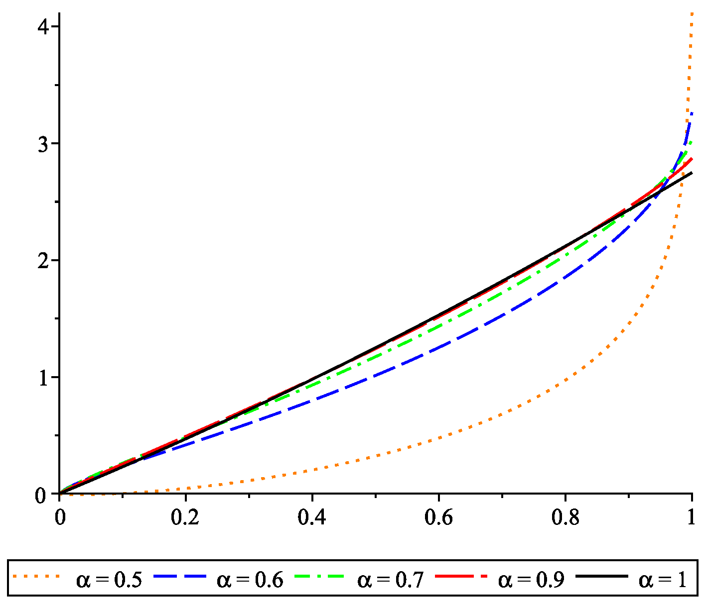
is the only candidate to be a local extremizer of functional $\tilde{\mathcal{J}}$, and, since $\tilde{\mathcal{J}}$ is jointly convex, $(\tilde{x},\tilde{\zeta })$ is the global minimizer. Solving the fractional problem analytically is very difficult, and thus a numerical technique is applied. In Figure 1, we show the results. Four different fractional orders are considered, and, as can be observed, the solution converges to $(\tilde{x},1)$ as α goes to one.

Example 2.

Suppose we intend to minimize

$$\mathcal{J}(x,\zeta )=$$

$$\frac{1}{2}{\int }_0^1\left(({(}^C{D}_{1^{-}}^{\beta ,\psi }x)\left(t\right)-\frac{{(\psi \left(1\right)-\psi \left(t\right))}^{1-\beta }}{\Gamma (2-\beta )}{)}^2+t^2-3+{(x\left(0\right)-1)}^2+{(\zeta -2)}^2\right)dt$$

in the class of functions $C^1([0,1],\mathbb{R})$, subject to the restriction $x\left(1\right)=0$ ($x\left(0\right)$ is free). From Theorem 3 every local extremizer of functional $\mathcal{J}$ satisfies the following necessary conditions:

• $\left(D_{0^{+}}^{\beta ,\psi }\frac{{}^C{D}_{1^{-}}^{\beta ,\psi }x-\frac{{(\psi \left(1\right)-\psi )}^{1-\beta }}{\Gamma (2-\beta )}}{{\psi }^{\prime }}\right)\left(t\right){\psi }^{\prime }\left(t\right)=0,t\in [0,1]$;
• ${\displaystyle {\int }_0^1(\zeta -2)dt=0}$;
• ${\displaystyle {\int }_0^1(x\left(0\right)-1)dt=-\left(I_{0^{+}}^{1-\beta ,\psi }\frac{{}^C{D}_{1^{-}}^{\beta ,\psi }x-\frac{{(\psi \left(1\right)-\psi )}^{1-\beta }}{\Gamma (2-\beta )}}{{\psi }^{\prime }}\right)\left(0\right).}$

Observe that the function $x:[0,1]\to \mathbb{R}$ defined by

$$x\left(t\right)=\psi \left(1\right)-\psi \left(t\right)$$

is such that

$${}^C{D}_{1^{-}}^{\beta ,\psi }x\left(t\right)={}^C{D}_{1^{-}}^{\beta ,\psi }(\psi \left(1\right)-\psi \left(t\right))={\displaystyle \frac{1}{\Gamma (2-\beta )}}{(\psi \left(1\right)-\psi \left(t\right))}^{1-\beta },$$

hence, x satisfies the Euler–Lagrange equation given in 1. Moreover, x satisfies the natural boundary condition given by 3 if $x\left(0\right)=1$, that is,

$$\psi \left(1\right)=1+\psi \left(0\right).$$

(35)

We remark that if $\psi =Id$, then we are dealing with the Caputo derivative and the identity (35) holds. Hence,

$$(x^{🟉},{\zeta }^{🟉})=(\psi \left(1\right)-\psi \left(t\right),2)$$

is a possible local minimizer of functional $\mathcal{J}$. Observing that, for every function $C^1([0,1],\mathbb{R})$, we have

$$\mathcal{J}(x,\zeta )\ge \frac{1}{2}{\int }_0^1(t^2-3)dt=-\frac{4}{3}$$

and since $\mathcal{J}(x^{🟉},{\zeta }^{🟉})=-\frac{4}{3}$, then $(x^{🟉},{\zeta }^{🟉})$ is indeed a global minimizer of $\mathcal{J}$.

Example 3.

The goal is to minimize

$$\mathcal{J}(x,\zeta )={\int }_0^1\left(\frac{{(\psi \left(t\right)-\psi \left(0\right))}^{\alpha }}{2\Gamma (2+\alpha )}{{(}^C{D}_{0^{+}}^{\alpha ,\psi }x)}^2\left(t\right)-{(}^C{D}_{0^{+}}^{\alpha ,\psi }x)\left(t\right){(\psi \left(t\right)-\psi \left(0\right))}^{\alpha +1}\right)dt$$

in the class of functions $C^1([0,1],\mathbb{R})$, subject to the restriction $x\left(0\right)=0$ ($x\left(1\right)$ is free) and to the integral constraint

$$\mathcal{I}(x,\zeta )={\int }_0^1({(x\left(1\right)-2)}^2+{(\zeta -1)}^2)dt=0.$$

(36)

We assume that the kernel fulfills the condition $\psi \left(1\right)=\psi \left(0\right)+2^{\frac{1}{\alpha +1}}$. Fix $({\lambda }_0,\lambda )\in {\mathbb{R}}^2\backslash \left\{(0,0)\right\}$ and define

$$\begin{array}{c}M:={\lambda }_0\left(\frac{{(\psi \left(t\right)-\psi \left(0\right))}^{\alpha }}{2\Gamma (2+\alpha )}{{(}^C{D}_{0^{+}}^{\alpha ,\psi }x)}^2\left(t\right)-{(}^C{D}_{0^{+}}^{\alpha ,\psi }x)\left(t\right){(\psi \left(t\right)-\psi \left(0\right))}^{\alpha +1}\right)\hfill \\ \hfill +\lambda \left({(x\left(1\right)-2)}^2+{(\zeta -1)}^2\right).\end{array}$$

From Theorem 6, every local extremizer of functional $\mathcal{J}$ subject to the integral constraint (36) satisfies the following conditions:

• ${\lambda }_0\left(D_{1^{-}}^{\alpha ,\psi }\frac{\frac{{(\psi -\psi \left(0\right))}^{\alpha }}{\Gamma (2+\alpha )}{(}^C{D}_{0^{+}}^{\alpha ,\psi }x)-{(\psi -\psi \left(0\right))}^{\alpha +1}}{{\psi }^{\prime }}\right)\left(t\right){\psi }^{\prime }\left(t\right)=0,t\in [0,1]$;
• ${\displaystyle \lambda {\int }_0^{1}2(\zeta -1)dt=0}$;
• ${\displaystyle \lambda {\int }_0^{1}2(x\left(1\right)-2)dt=-{\lambda }_0\left(I_{1^{-}}^{1-\alpha ,\psi }\frac{\frac{{(\psi -\psi \left(0\right))}^{\alpha }}{\Gamma (2+\alpha )}{(}^C{D}_{0^{+}}^{\alpha ,\psi }x)-{(\psi -\psi \left(0\right))}^{\alpha +1}}{{\psi }^{\prime }}\right)\left(1\right).}$

Define $({\lambda }_0,\lambda )=(1,1)$ and $x^{🟉}:[0,1]\to \mathbb{R}$ by $x^{🟉}\left(t\right)={(\psi \left(t\right)-\psi \left(0\right))}^{\alpha +1}$. In this case,

$${(}^C{D}_{0^{+}}^{\alpha ,\psi }{x}^{🟉})\left(t\right)=\Gamma (2+\alpha )(\psi \left(t\right)-\psi \left(0\right))$$

and, therefore,

$$\frac{{(\psi \left(t\right)-\psi \left(0\right))}^{\alpha }}{\Gamma (2+\alpha )}{(}^C{D}_{0^{+}}^{\alpha ,\psi }{x}^{🟉})\left(t\right)-{(\psi \left(t\right)-\psi \left(0\right))}^{\alpha +1}=0.$$

Hence, $(x^{🟉},1)$ satisfies the integral constraint (36) and the necessary conditions 1–3.

4. Conclusions and Future Work

In this work, we proved necessary and sufficient conditions of optimality, where the Lagrangian function depends on a general form of fractional derivative, a free parameter, and the state values. The Euler–Lagrange equation was deduced, for the fundamental problem, as well when in presence of constraints. With some examples, we show the applicability of the procedure.

For future, direct methods can be studied to deal with such generalized fractional variational problems. One possible direction is to study discretizations of the fractional derivative and then convert the problem as a finite dimensional case. In addition, other optimization conditions could be obtained, e.g., with arbitrary fractional orders $\alpha ,\beta \in {\mathbb{R}}^{+}$, or optimal control problems where the state equation involves the $\psi$-Caputo fractional derivative.

References

- Podlubny, I. Fractional Differential Equations; Academic Press: San Diego, CA, USA, 1999. [Google Scholar]
- Samko, S.G.; Kilbas, A.A.; Marichev, O.I. Fractional Integrals and Derivatives, Translated from the 1987 Russian Original; Gordon and Breach: Yverdon, Switzerland, 1993. [Google Scholar]
- Hilfer, R. Applications of Fractional Calculus in Physics; World Scientific: Singapore, 2000. [Google Scholar]
- Holm, S.; Sinkus, R. A unifying fractional wave equation for compressional and shear waves. J. Acoust. Soc. Am. 2010, 127, 542–548. [Google Scholar] [CrossRef] [Green Version]
- Machado, J.A.T. Discrete-time fractional-order controllers. Fract. Calc. Appl. Anal. 2001, 4, 47–66. [Google Scholar]
- Žecová, M.; Terpxaxk, J. Heat conduction modeling by using fractional-order derivatives. Appl. Math. Comput. 2015, 257, 365–373. [Google Scholar] [CrossRef] [Green Version]
- Pu, Y.F. Fractional differential analysis for texture of digital image. J. Alg. Comput. Technol. 2007, 1, 357–380. [Google Scholar]
- Magin, R.L. Fractional calculus in bioengineering. Crit. Rev. Biomed. Eng. 2004, 32, 1–104. [Google Scholar] [CrossRef] [PubMed] [Green Version]
- Pinto, C.M.A.; Carvalho, A.R.M. Fractional order model for HIV dynamics. J. Comput. Appl. Math. 2017, 312, 240–256. [Google Scholar] [CrossRef]
- Chen, L.; Hu, F.; Zhu, W. Stochastic dynamics and fractional optimal control of quasi integrable Hamiltonian systems with fractional derivative damping. Fract. Calc. Appl. Anal. 2013, 16, 189–225. [Google Scholar] [CrossRef]
- Mophou, G.M. Optimal control of fractional diffusion equation. Comput. Math. Appl. 2011, 61, 68–78. [Google Scholar] [CrossRef] [Green Version]
- Saeedian, M.; Khalighi, M.; Azimi–Tafreshi, N.; Jafari, G.R.; Ausloos, M. Memory effects on epidemic evolution: The susceptible-infected-recovered epidemic model. Phys. Rev. E 2017, 95, 022409. [Google Scholar] [CrossRef] [Green Version]
- Škovránek, T.; Podlubny, I.; Petrxaxš, I. Modeling of the national economies in state-space: A fractional calculus approach. Econ. Model. 2012, 29, 1322–1327. [Google Scholar] [CrossRef]
- Almeida, R. A Caputo fractional derivative of a function with respect to another function. Commun. Nonlinear Sci. Numer. Simul. 2017, 44, 460–481. [Google Scholar] [CrossRef] [Green Version]
- Riewe, F. Nonconservative Lagrangian and Hamiltonian mechanics. Phys. Rev. E 1996, 53, 1890–1899. [Google Scholar] [CrossRef]
- Riewe, F. Mechanics with fractional derivatives. Phys. Rev. E 1997, 55, 3581–3592. [Google Scholar] [CrossRef]
- Almeida, R.; Pooseh, S.; Torres, D.F.M. Computational Methods in the Fractional Calculus of Variations; Imperial College Press: London, UK, 2015. [Google Scholar]
- Malinowska, A.B.; Odzijewicz, T.; Torres, Ḋ.F.M. Advanced Methods in the Fractional Calculus of Variations, SpringerBriefs in Applied Sciences and Technology; Springer: Cham, Switzerland, 2015. [Google Scholar]
- Malinowska, A.B.; Torres, D.F.M. Introduction to the Fractional Calculus of Variations; Imperial College Press: London, UK, 2012. [Google Scholar]
- Atanacković, T.M.; Konjik, S.; Pilipović, Ṡ. Variational problems with fractional derivatives: Euler-Lagrange equations. J. Phys. A 2008, 41, 095201. [Google Scholar] [CrossRef]
- Baleanu, D.; Muslih, S.I.; Rabei, E.M. On fractional Euler–Lagrange and Hamilton equations and the fractional generalization of total time derivative. Nonlinear Dynam. 2008, 53, 67–74. [Google Scholar] [CrossRef] [Green Version]
- Bourdin, L.; Odzijewicz, T.; Torres, Ḋ.F.M. Existence of minimizers for fractional variational problems containing Caputo derivatives. Adv. Dyn. Syst. Appl. 2013, 8, 3–12. [Google Scholar]
- Herzallah, M.A.E.; Baleanu, D. Fractional-order Euler-Lagrange equations and formulation of Hamiltonian equations. Nonlinear Dynam. 2009, 58, 385–391. [Google Scholar] [CrossRef]
- Klimek, M. Lagrangean and Hamiltonian fractional sequential mechanics. Czechoslov. J. Phys. 2002, 52, 1247–1253. [Google Scholar] [CrossRef]
- Agrawal, O.P. Formulation of Euler-Lagrange equations for fractional variational problems. J. Math. Anal. Appl. 2002, 272, 368–379. [Google Scholar] [CrossRef] [Green Version]
- Agrawal, O.P. Fractional variational calculus and the transversality conditions. J. Phys. A 2006, 39, 10375–10384. [Google Scholar] [CrossRef]
- Almeida, R. Optimality conditions for fractional variational problems with free terminal time. Discrete Contin. Dyn. Syst. Ser. S 2018, 11, 1–19. [Google Scholar] [CrossRef]
- Zinober, A.; Sufahani, S. A non-standard optimal control problem arising in an economics application. Pesqui. Oper. 2013, 33, 63–71. [Google Scholar] [CrossRef] [Green Version]
- Hoffman, K.A. Stability results for constrained calculus of variations problems: An analysis of the twisted elastic loop. Proc. R. Soc. A Math. Phys. Eng. Sci. 2005, 461, 1357–1381. [Google Scholar] [CrossRef]
- Malinowska, A.B.; Torres, D.F.M. Generalized natural boundary conditions for fractional variational problems in terms of the Caputo derivative. Comput. Math. Appl. 2010, 59, 3110–3116. [Google Scholar] [CrossRef] [Green Version]
- Martins, N. A non-standard class of variational problems of Herglotz type. Discrete Contin. Dyn. Syst. 2021, in press. [Google Scholar]
- Van Brunt, B. The Calculus of Variations, Universitext; Springer: New York, NY, USA, 2004. [Google Scholar]
- Agrawal, O.P. Generalized Euler-Lagrange equations and transversality conditions for FVPs in terms of the Caputo derivative. J. Vib. Control 2007, 13, 1217–1237. [Google Scholar] [CrossRef]
- Almeida, R.; Ferreira, R.A.C.; Torres, D.F.M. Isoperimetric problems of the calculus of variations with fractional derivatives. Acta Math. Sci. Ser. B Engl. 2012, 32, 619–630. [Google Scholar] [CrossRef] [Green Version]
Figure 1.
Numerical solutions for Example 1.
Publisher’s Note: MDPI stays neutral with regard to jurisdictional claims in published maps and institutional affiliations. |
© 2021 by the authors. Licensee MDPI, Basel, Switzerland. This article is an open access article distributed under the terms and conditions of the Creative Commons Attribution (CC BY) license (http://creativecommons.org/licenses/by/4.0/).
Share and Cite
MDPI and ACS Style
Almeida, R.; Martins, N. A Generalization of a Fractional Variational Problem with Dependence on the Boundaries and a Real Parameter. Fractal Fract. 2021, 5, 24. https://0-doi-org.brum.beds.ac.uk/10.3390/fractalfract5010024
AMA Style
Almeida R, Martins N. A Generalization of a Fractional Variational Problem with Dependence on the Boundaries and a Real Parameter. Fractal and Fractional. 2021; 5(1):24. https://0-doi-org.brum.beds.ac.uk/10.3390/fractalfract5010024
Chicago/Turabian StyleAlmeida, Ricardo, and Natália Martins. 2021. "A Generalization of a Fractional Variational Problem with Dependence on the Boundaries and a Real Parameter" Fractal and Fractional 5, no. 1: 24. https://0-doi-org.brum.beds.ac.uk/10.3390/fractalfract5010024