Extraction Complex Properties of the Nonlinear Modified Alpha Equation


1
Department of Mathematics and Science Education, Faculty of Education, Harran University, Sanliurfa 63510, Turkey
2
Faculty of Arts and Sciences, Harran University, Sanliurfa 63510, Turkey
*
Author to whom correspondence should be addressed.
Fractal Fract. 2021, 5(1), 6; https://0-doi-org.brum.beds.ac.uk/10.3390/fractalfract5010006
Submission received: 13 November 2020
/
Revised: 7 December 2020
/
Accepted: 31 December 2020
/
Published: 7 January 2021
(This article belongs to the Special Issue New Challenges Arising in Engineering Problems with Fractional and Integer Order)
Abstract
:This paper applies one of the special cases of auxiliary method, which is named as the Bernoulli sub-equation function method, to the nonlinear modified alpha equation. The characteristic properties of these solutions, such as complex and soliton solutions, are extracted. Moreover, the strain conditions of solutions are also reported in detail. Observing the figures plotted by considering various values of parameters of these solutions confirms the effectiveness of the approximation method used for the governing model.
1. Introduction
In the last three decades, we have seen an enthralling research topic on the real world problems expressed by using mathematical models. Qi et al. have investigated some important models used to describe the certain waves in physics [1,2]. In this sense, an interesting model for investigating numerically the nonlinear weakly singular models has been presented by Ray et al. [3]. Syam has worked on the Bernoulli sub-equation method [4]. He has also obtained a lot of different interesting results for the governing model. A few years ago, Mendo has studied the series of wave forces connected with Bernoulli structures [5]. He has also produced a different Bernoulli variable algorithm. Rani et al. have studied on a special matrix that could be solved by Bernoulli polynomials [6]. Jeon et al. have investigated the generalized hypergeometric differential [7]. In 2019, Arqub et al. have studied the Riccati and Bernoulli properties to find new and different solutions for the governing model [8]. Ordokhani et al. have observed some important properties the Bernoulli wavelets with their special cases [9]. Yang has proved a new form of high order Bernoulli polynomials in 2008 [10], which obtained many new special cases about the Bernoulli model. In 2016, Dilcher has searched for identities of the Bernoulli polynomial properties in a physical aspect [11,12]. Furthermore, they have given more detailed information regarding these special functions. Ordokhani et al. have defined an original rational relation based on the Bernoulli wavelet [13]. Tian et al. have worked on the solution of beam problem by using an ansatz method based on the Bernoulli polinomials [14], and so on [15,16,17,18,19,20,21,22,23,24,25,26,27].
More general properties of auxiliary and sub-equation function methods have been comprehensively introduced in the literature [28,29]. Moreover, there are many published methods for solving similar equations using different techniques and methods [30,31,32,33,34,35,36,37,38,39,40,41,42,43,44,45,46,47,48,49].
In the organization of this paper, in Section 2, we give some preliminaries about the method. In Section 3, we discuss the application of projected method to the nonlinear modified alpha equation (MAE) defined as [21]
in which is real constant and non-zero. Islam et al., have applied the modified simple equation method to Equation (1) for getting some important properties [21]. Wazwaz investigated the physical meaning of Equation (1) in a previous study [22].
Comparison and discussion related to the solutions obtained in this paper are presented in Section 4. After the graphical simulations, a conclusion completes the paper.
2. Fundamental Facts of BSEFM
This section presents the general properties of BSEFM [23] based on the four steps defined as follows:
Step 1. We consider the following nonlinear partial differential equation (NLPDE) given as
which is taking into account the travelling wave transformation
where . Substituting Equation (3) into Equation (2) yields the following ordinary differential equation:
Step 2. In this step, we take the following trial solution equation to the Equation (4):
and
where is Bernoulli differential polynomial. Substituting Equation (5) along with Equation (6) into Equation (4), it produces an algebraic equation of polynomial as follows:
We can find more than one solution by obtaining a relation between and via the balancing principle and then using this relation.
Step 3. If we take into account that all the coefficients of are zero:
If we solve this system, we will find and control the values of
Step 4. Solving Equation (6), we find the following according to and :
Using a complete discrimination system for polynomial parameters, we find the solutions to Equation (4), using some computational programs, and organize the exact solutions to Equation (4). In order to better understand the results obtained in this way, we can draw the two and three dimensional surfaces of the solutions by considering the appropriate parameter values.
3. Implementation of the BSEFM
This section of the manuscript applies the BSEFM to the MAE to obtain new complex and exponential solutions. Using
where are real constants and non-zero, we obtain the nonlinear ordinary equation as follows:
With the help of the balance principle, it is obtained a relationship between and as follows:
This gives some new analytical solutions for the governing model being Equation (1).
Case 1: Considering as and produce the following trial solution for Equation (10):
and
where Putting Equations (12)–(14) into Equation (10), it gives a system of algebraic equations of . With the help of powerful computational programs, we get the following coefficients and solutions.
Case 1.1. If it is selected follows:
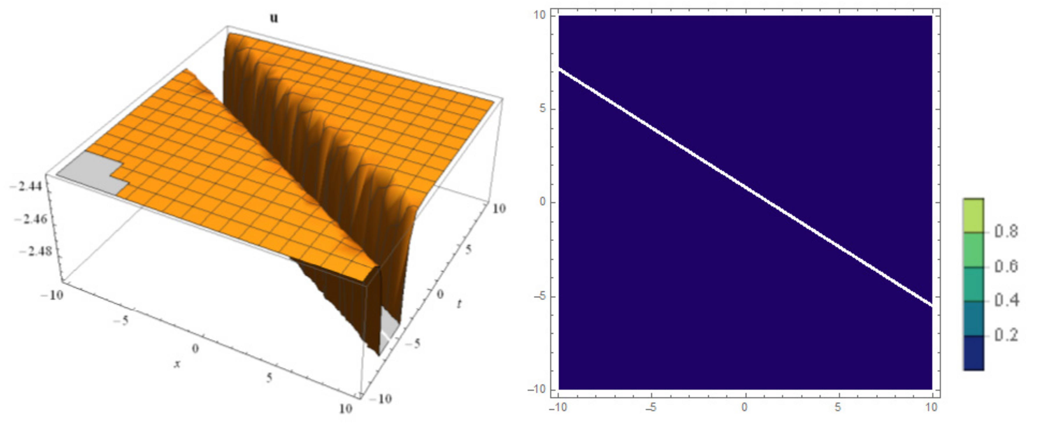
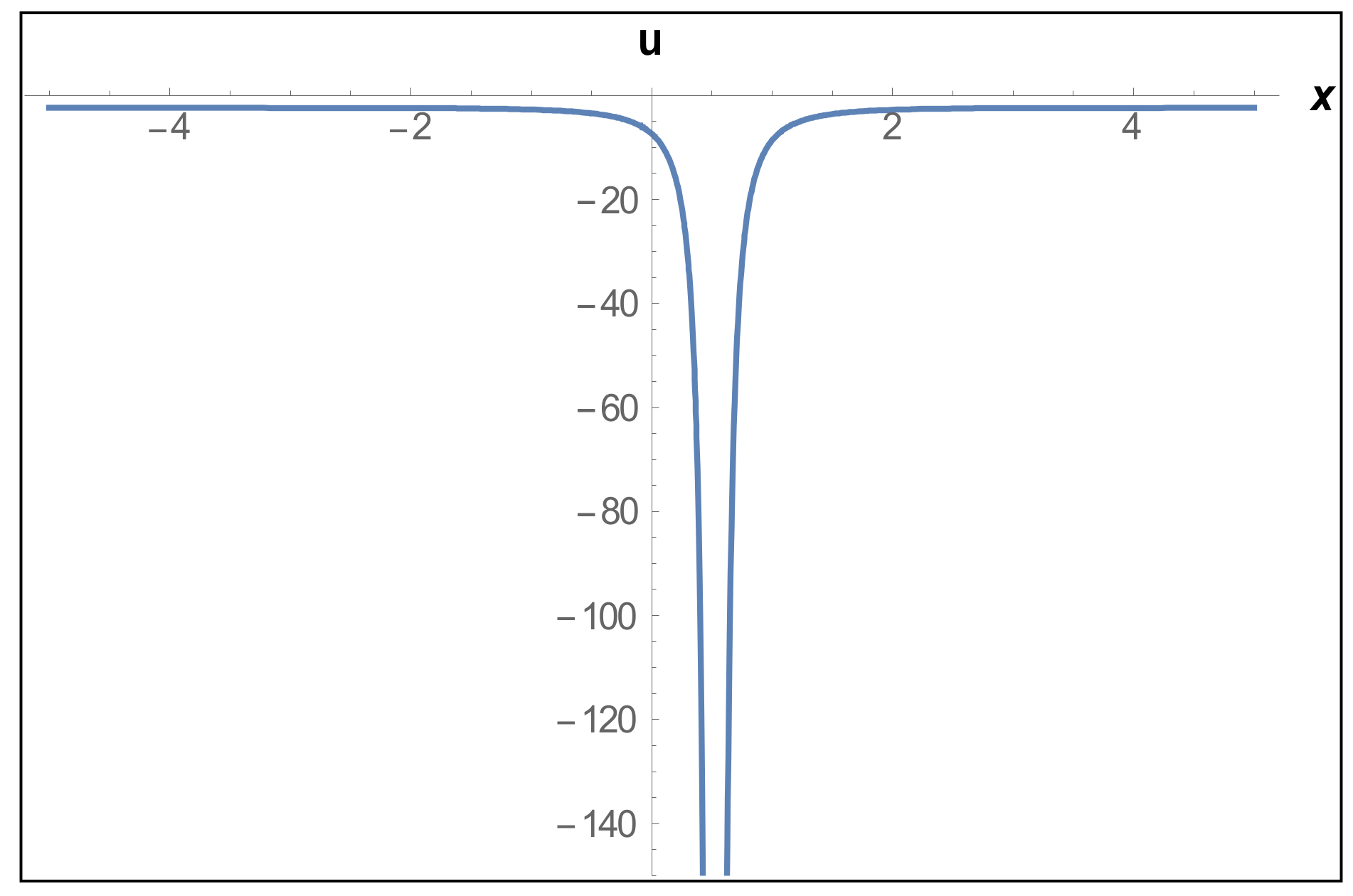
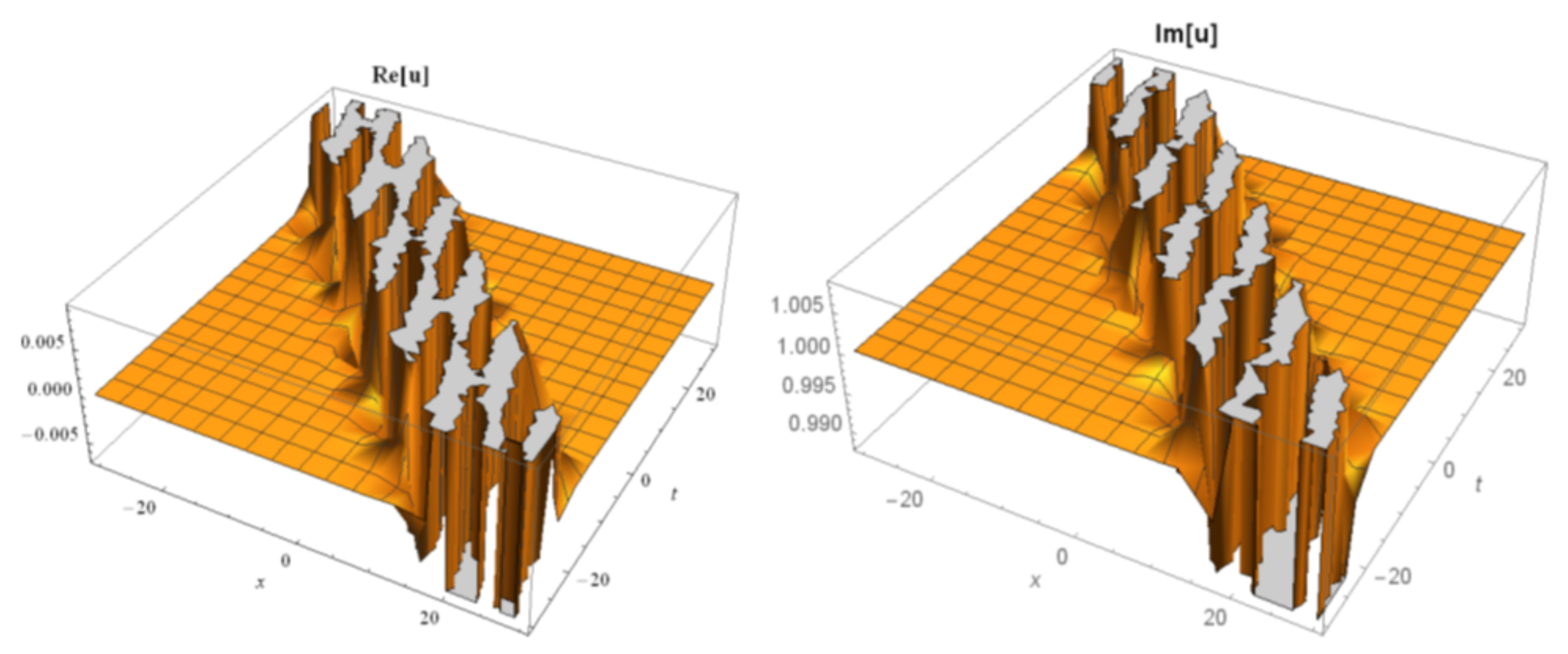
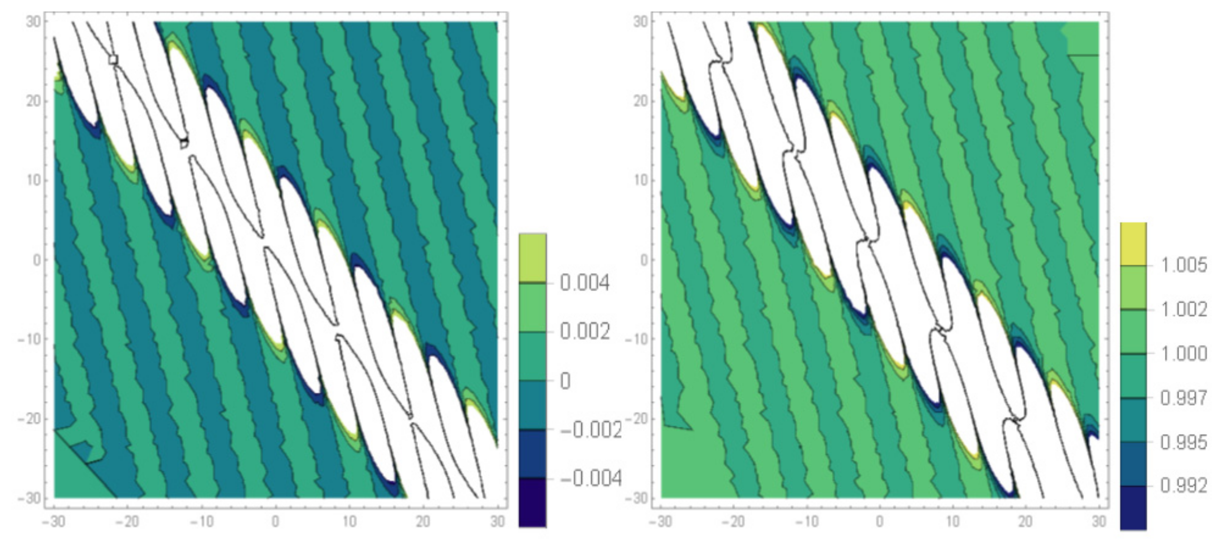
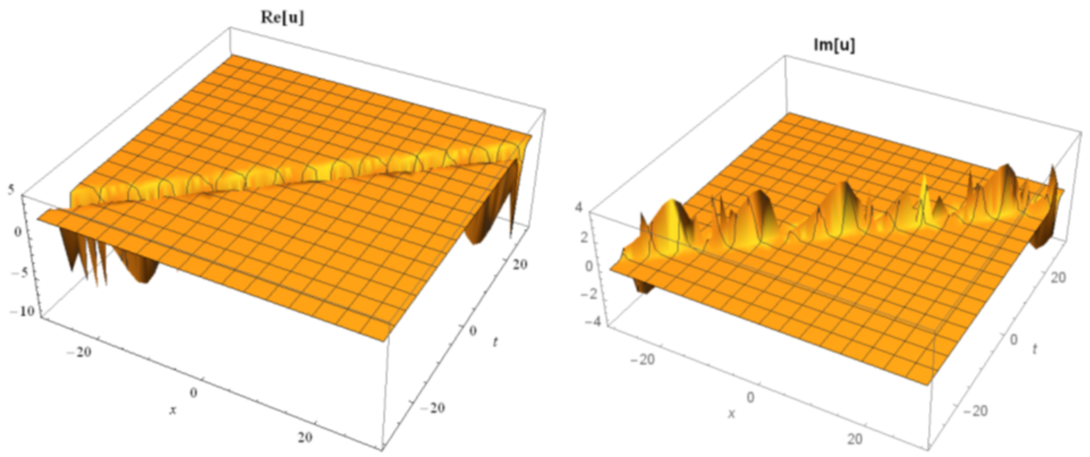
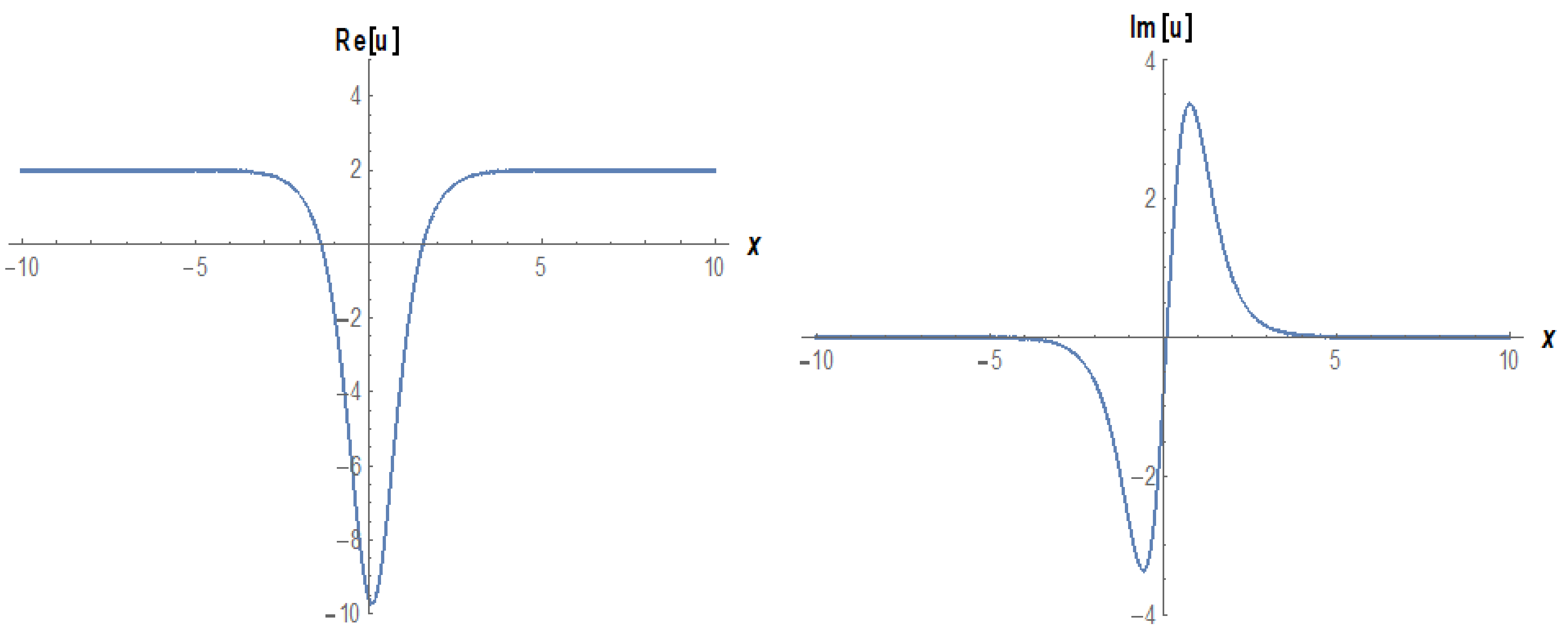
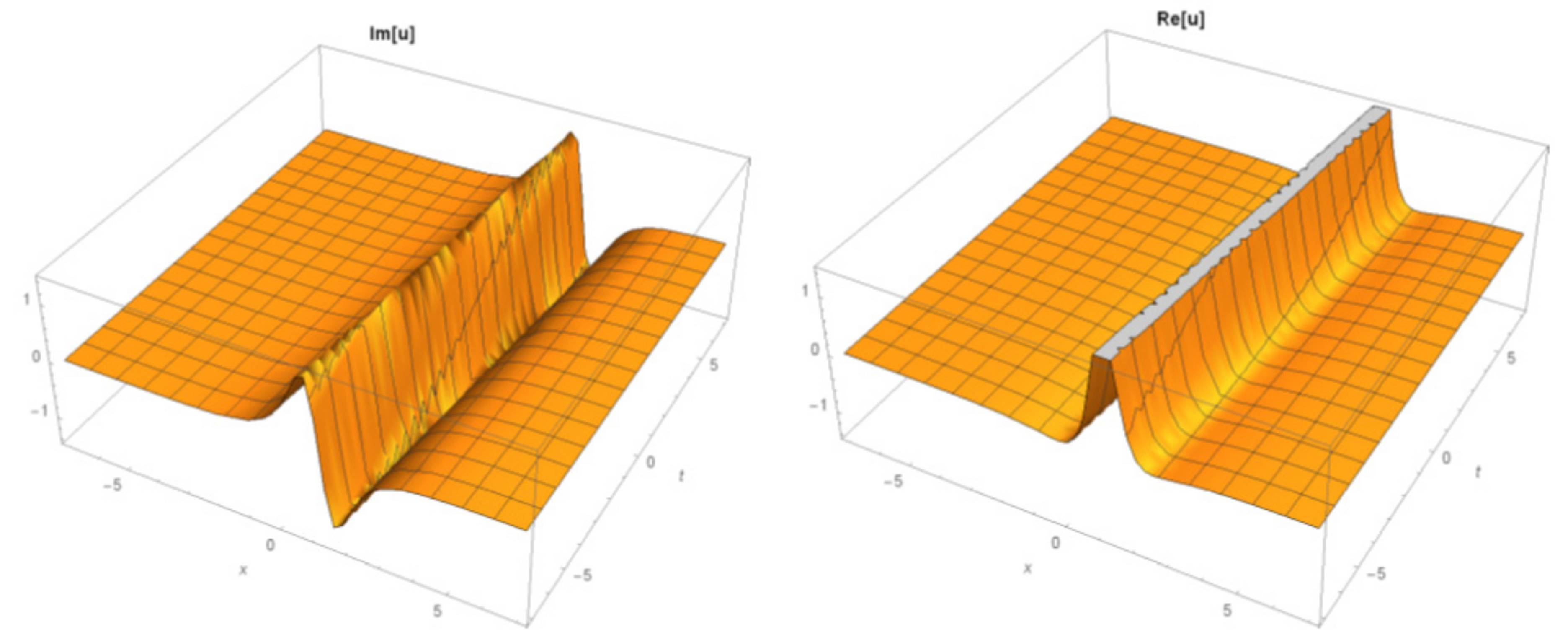
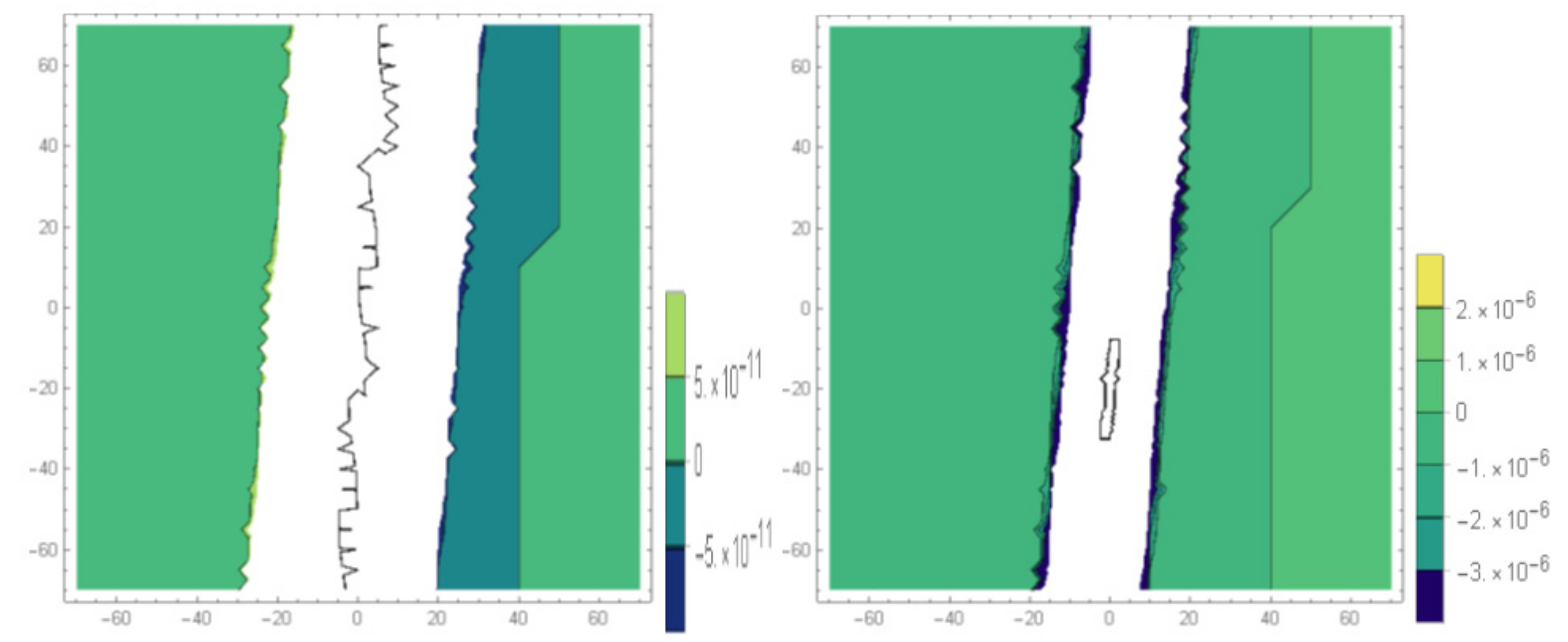
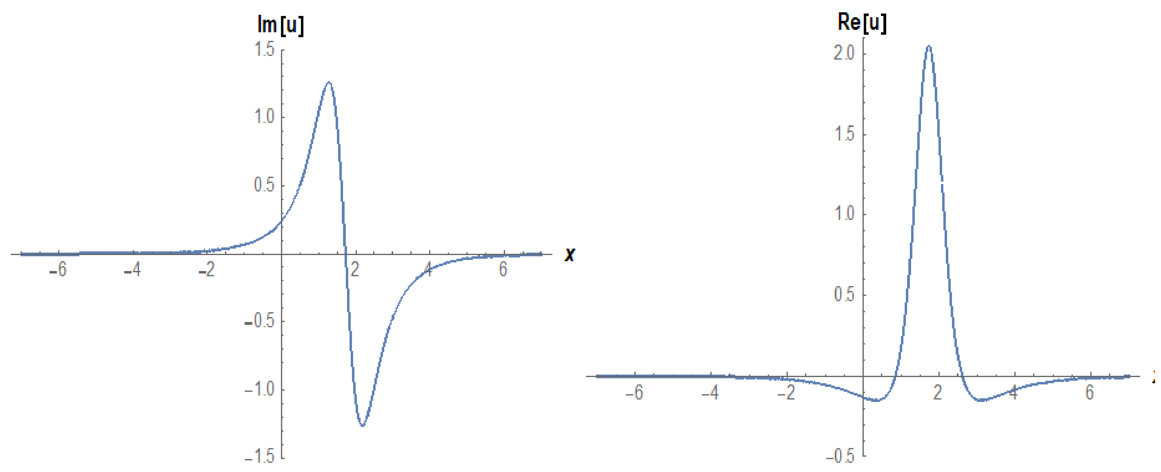
we find the following new singular soliton solution for the governing model being Equation (1):
in which
for validity of Equation (16). Choosing the suitable values of parameters in Equation (16), we plot various figures as follows as being in Figure 1 and Figure 2.
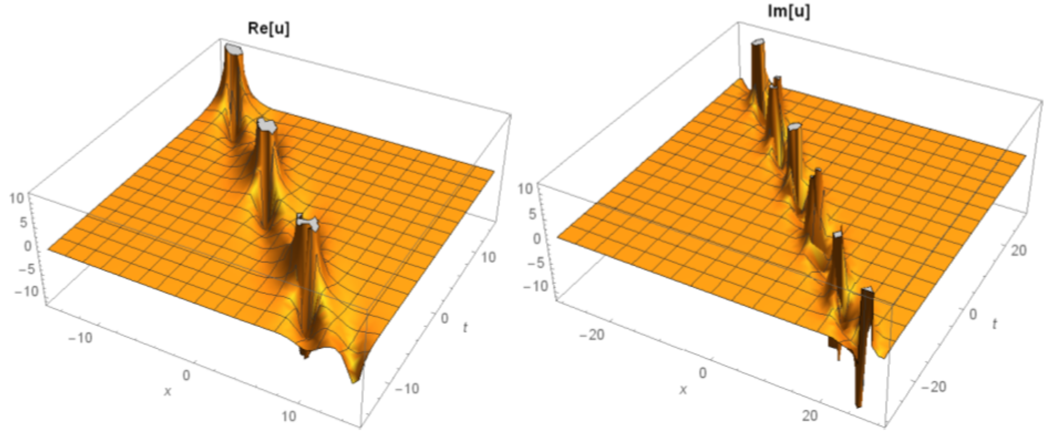
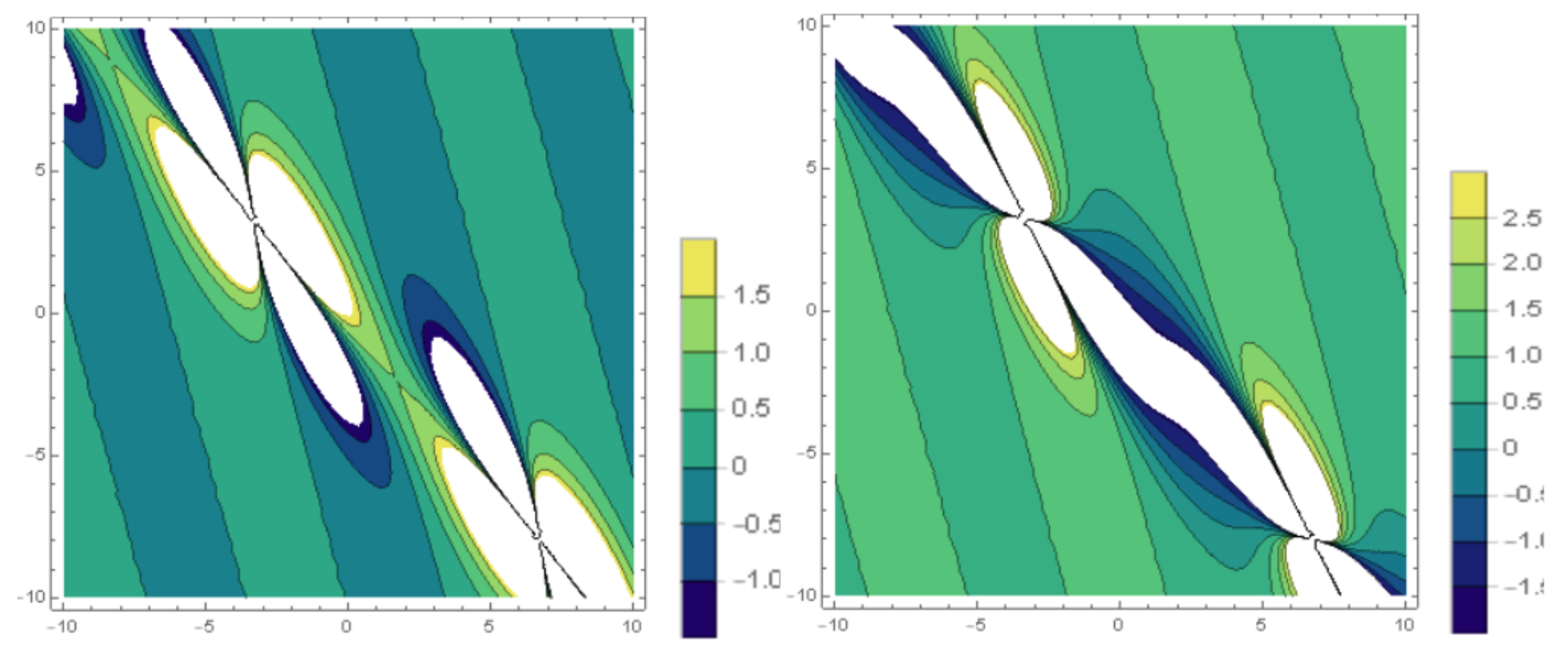
Case 1.2. For , when they are considered as follows:
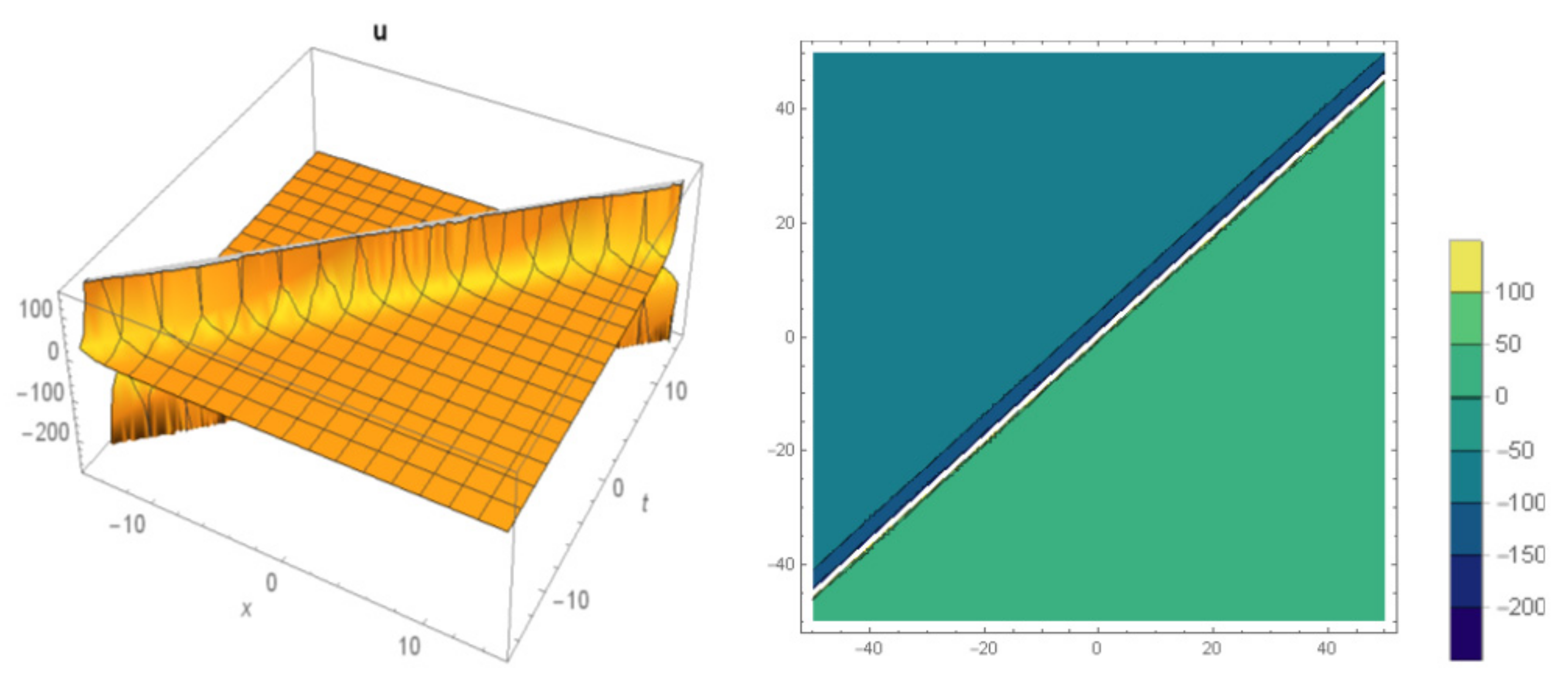
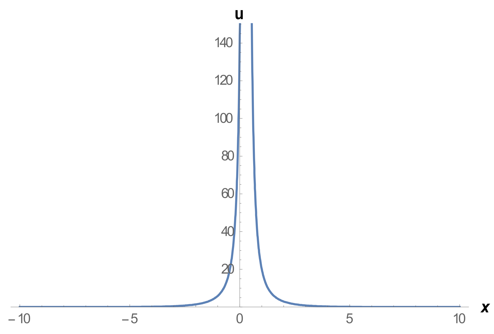
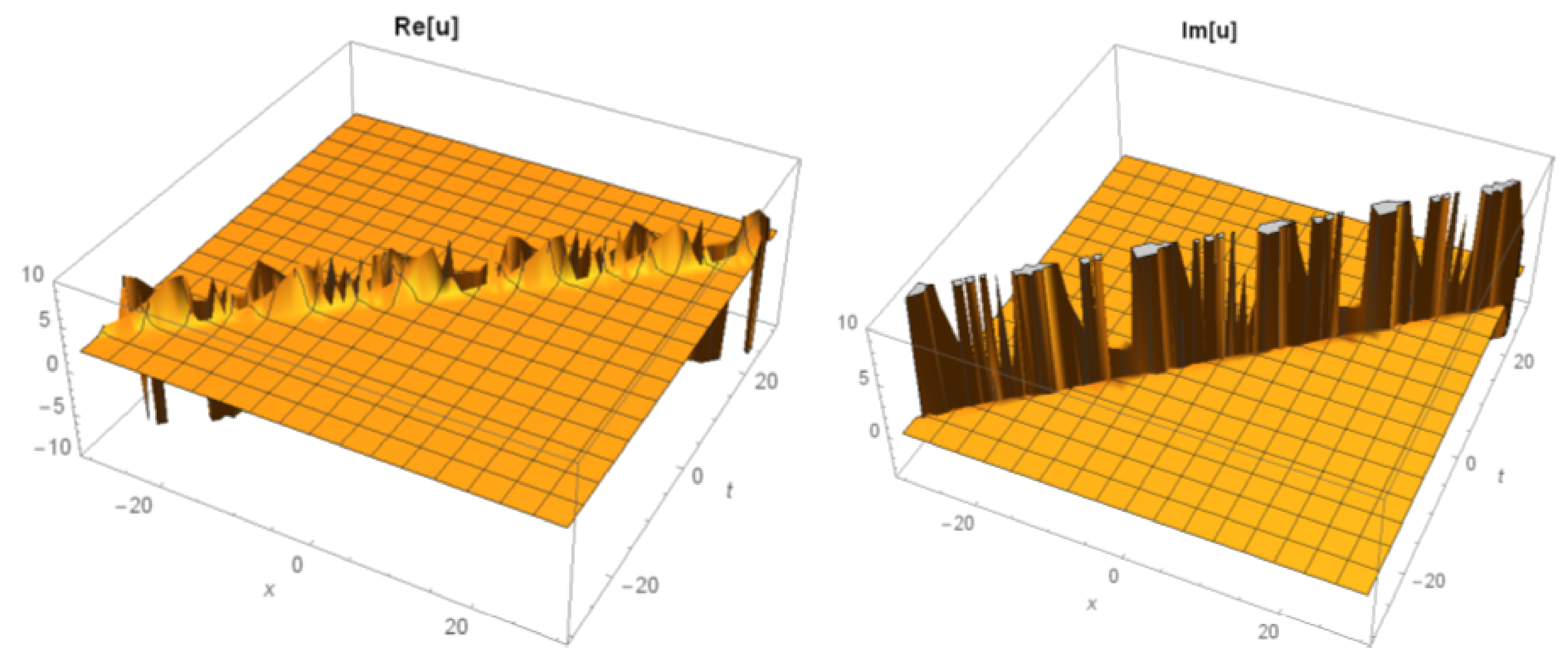
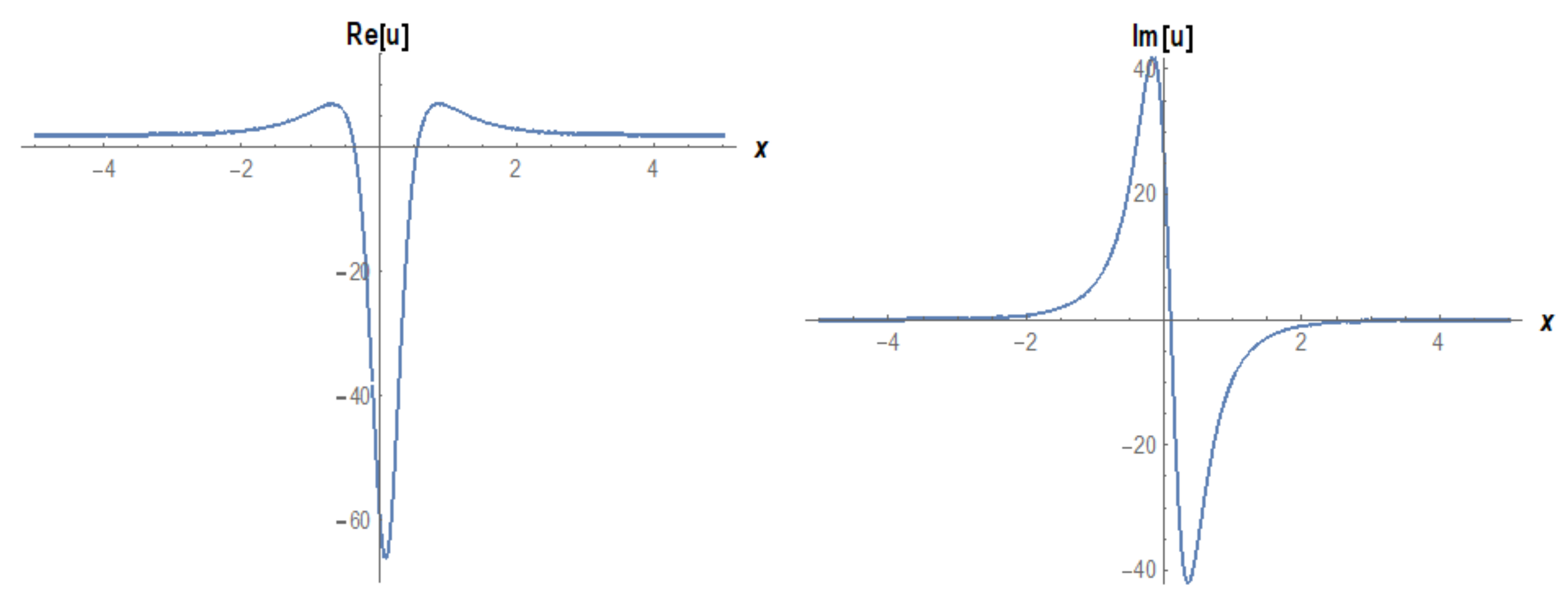
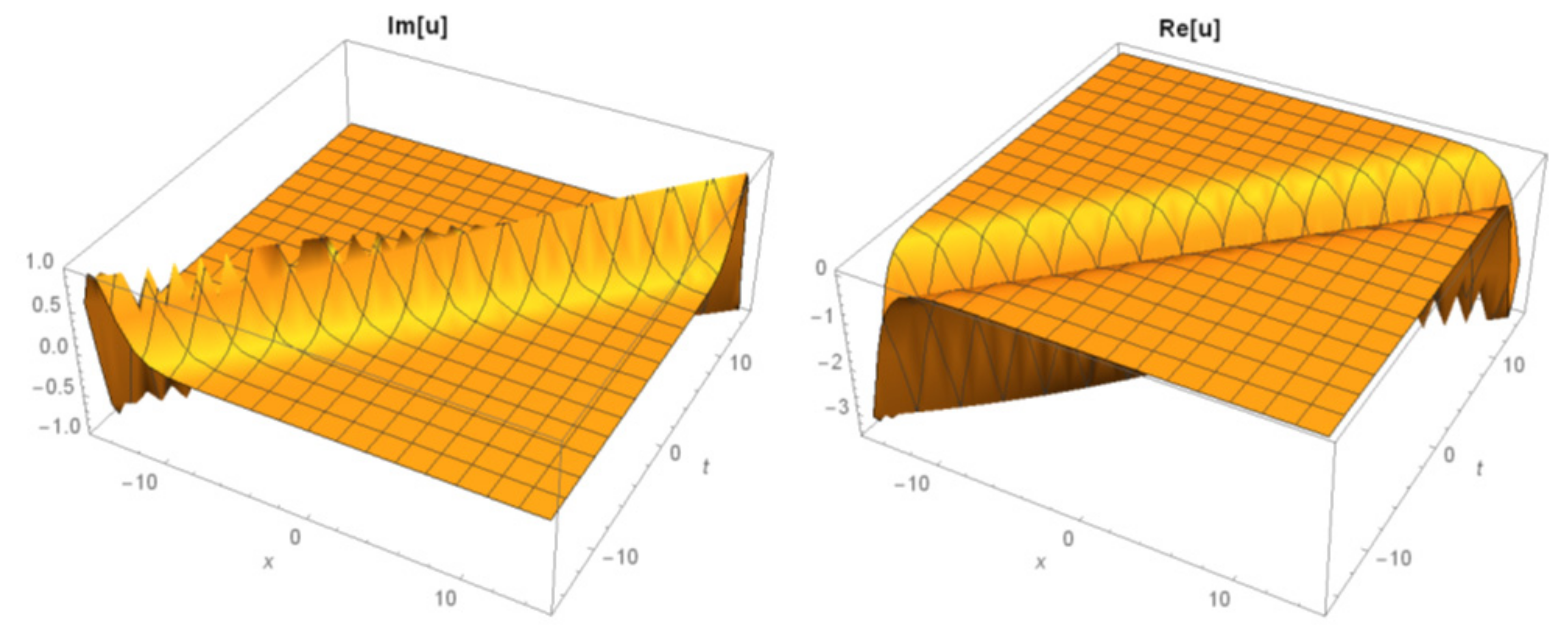
This produces a new singular soliton solution for the governing model as:
The strain condition is also given as . We can observe the wave surfaces of Equation (18) as being in Figure 3 and Figure 4.
Case 1.3. If we select the following complex coefficient together with ,
it produces a complex soliton solution for the governing model as:
Case 1.4. When choosing the following other complex coefficients and also ,
it produces another complex soliton solution to the governing model as:
Under the suitable choosing of the values of these parameters, we plot various graphs as being Figure 8, Figure 9 and Figure 10.
Case 1.5. Choosing the following other complex coefficients by considering ,
gives another complex exponential function solution as:
Choosing the suitable values of these parameters, we present several simulations as Figure 11, Figure 12 and Figure 13.
Case 1.6. Taking the following other complex coefficients with ,
gives another complex exponential function solution as:
Case 2. Taking and , we can write as follows:
and
where . Putting Equations (27) and (28) into Equation (10) produces some entirely new analytical solutions for the governing model as follows.
Case 2.1: When
another new complex soliton solution is extracted as:
in which is a real constant with non-zero. Under the suitable chosen of parameters, we can presents various graphs as in Figure 17, Figure 18 and Figure 19.
Case 2.2. Considering the following:
another new complex mixed dark soliton solution is extracted as:
in which are real constants and non-zero and also
4. Comparison and Discussion
In a previous research [21], Asaduzzman et al., have studied the special cases of Equation (1) by considering . In this paper, we have extracted the general solutions of MAE according to as being in the solutions of Equations (16), (18), and (32). Moreover, we have also investigated other values of such as complex and rations in the coefficients of Equations (19), (21), (23), (25) and (29). When we compare these solutions with the solutions presented in the previous study [21], it may be observed that they are an entirely new solution for the governing model of MAE.
Moreover, if we consider more values of as and , we obtain another new solution for the governing model as:
in which . By getting the necessary derivations of Equation (33) for Equation (10), we report more new complex and rational wave solutions to the MAE, which these solutions produced by BSEFM. In this regard, this projected technique is a powerful tool for obtaining new analytical solutions for the nonlinear partial differential equations.
In the physical sense, if we consider the solution of being Equation (32), this is a complex mixed dark soliton solution for the governing model. Such reported results in this manuscript have some important properties. To illustrate this, the hyperbolic tangent (dark soliton) arises in the calculation of magnetic moment and rapidity of special relativity [50]. In this regard, it is estimated that this solution may help to better understanding of the meaning of MAE physically.
5. Conclusions
In this article, we have successfully applied BSEFM to the MAE. We obtained many entirely new complex and exponential characteristic properties of MAE. We observed that the results obtained with the help of the projected algorithm are new deeper investigations and a generalized version according to Moreover, we have reported the strain conditions for the validity of solutions. Various wave behaviors in many simulations from Figure 1, Figure 2, Figure 3, Figure 4, Figure 5, Figure 6, Figure 7, Figure 8, Figure 9, Figure 10, Figure 11, Figure 12, Figure 13, Figure 14, Figure 15, Figure 16, Figure 17, Figure 18, Figure 19, Figure 20, Figure 21 and Figure 22 have been also presented to observe wave distributions of solutions. All figures are clearly commented, which give the idea of effectiveness of the proposed schemes. The method proposed in this paper can be used to seek more travelling wave solutions of such governing models, because the method has some advantages such as easily calculations, writing programme for obtaining coefficients, and many others.
Author Contributions
The first Author has majorly contributed to the paper. Formal analysis, H.M.B.; Writing—original draft, M.E. All authors have read and agreed to the published version of the manuscript.
Funding
This research received no external funding.
Institutional Review Board Statement
Not applicable.
Informed Consent Statement
Not applicable.
Data Availability Statement
Data available in a publicly accessible repository.
Acknowledgements
This paper belongs to the Master’s thesis of the second author.
Conflicts of Interest
The authors declare no conflict of interest.
References
- Qi, F.-H.; Huang, Y.-H.; Wang, P. Solitary-wave and new exact solutions for an extended (3+1)-dimensional Jimbo–Miwa-like equation. Appl. Math. Lett. 2020, 100, 106004. [Google Scholar] [CrossRef]
- Cao, B. Solutions of Jimbo-Miwa Equation and Konopelchenko-Dubrovsky Equations. arXiv 2009, arXiv:0902.3308. [Google Scholar]
- Behera, S.; Ray, S.S. An operational matrix based scheme for numerical solutions of nonlinear weakly singular partial integro-differential equations. Appl. Math. Comput. 2020, 367, 124771. [Google Scholar] [CrossRef]
- Syam, M.I. The solution of Cahn-Allen equation based on Bernoulli sub-equation method. Results Phys. 2019, 14, 102413. [Google Scholar] [CrossRef]
- Mendo, L. An asymptotically optimal Bernoulli factory for certain functions that can be expressed as power series. Stoch. Process. Their Appl. 2019, 129, 4366–4384. [Google Scholar] [CrossRef] [Green Version]
- Rani, D.; Mishra, V. Numerical inverse Laplace transform based on Bernoulli polynomials operational matrix for solving nonlinear differential equations. Results Phys. 2020, 16, 102836. [Google Scholar] [CrossRef]
- Lee, J.Y.; Jeon, W. Exact solution of Euler-Bernoulli equation for acoustic black holes via generalized hypergeometric differential equation. J. Sound Vib. 2019, 452, 191–204. [Google Scholar] [CrossRef]
- Arqub, O.A.; Maayah, B. Modulation of reproducing kernel Hilbert space method for numerical solutions of Riccati and Bernoulli equations in the Atangana-Baleanu fractional sense. Chaos Solitons Fractals 2019, 125, 163–170. [Google Scholar]
- Rahimkhani, P.; Ordokhani, Y.; Babolian, E. Numerical solution of fractional pantograph differential equations by using generalized fractional-order Bernoulli wavelet. J. Comput. Appl. Math. 2017, 309, 493–510. [Google Scholar] [CrossRef]
- Yang, S.L. An identity of symmetry for the Bernoulli polynomials. Discret. Math. 2008, 308, 550–554. [Google Scholar]
- Dilcher, K.; Vignat, C. General convolution identities for Bernoulli and Euler polynomials. J. Math. Anal. Appl. 2016, 435, 1478–1498. [Google Scholar]
- Dilcher, K.; Straub, A.; Vignat, C. Identities for Bernoulli polynomials related to multiple Tornheim zeta functions. J. Math. Anal. Appl. 2019, 476, 569–584. [Google Scholar] [CrossRef] [Green Version]
- Rahimkhani, P.; Ordokhani, Y.; Babolian, E. Fractional-order Bernoulli wavelets and their applications. Appl. Math. Model. 2016, 40, 8087–8107. [Google Scholar] [CrossRef]
- Ren, Q.; Tian, H. Numerical solution of the static beam problem by Bernoulli collocation method. Appl. Math. Model. 2016, 40, 8886–8897. [Google Scholar] [CrossRef] [Green Version]
- Jamei, M.M.; Beyki, M.R.; Koepf, W. An extension of the Euler-Maclaurin quadrature formula using a parametric type of Bernoulli polynomials. Bull. Des. Sci. Mathématiques 2019, 156, 102798. [Google Scholar]
- Rahimkhani, P.; Ordokhani, Y.; Babolian, E. Fractional-order Bernoulli functions and their applications in solving fractional Fredholem–Volterra integro-differential equations. Appl. Numer. Math. 2017, 122, 66–81. [Google Scholar] [CrossRef]
- Biswas, A.; Mirzazade, M.; Triki, H.; Zhou, Q.; Ullah, M.Z.; Moshokoa, S.P.; Belic, M. Perturbed resonant 1-soliton solution with an-ti-cubic nonlinearity by Riccati-Bernoulli sub-ODE method. Optik 2018, 156, 346–350. [Google Scholar]
- Keshavarz, E.; Ordokhani, Y.; Razzaghi, M. The Bernoulli wavelets operational matrix of integration and its applications for the solution of linear and nonlinear problems in calculus of variations. Appl. Math. Comput. 2019, 351, 83–98. [Google Scholar] [CrossRef]
- Zeghdane, R. Numerical solution of stochastic integral equations by using Bernoulli operational matrix. Math. Comput. Simul. 2019, 165, 238–254. [Google Scholar]
- Marinov, T.T.; Vatsala, A.S. Inverse problem for coefficient identification in the Euler–Bernoulli equation. Comput. Math. Appl. 2008, 56, 400–410. [Google Scholar] [CrossRef] [Green Version]
- Islam, N.; Asaduzzaman, M.; Ali, S. Exact wave solutions to the simplified modified Camassa-Holm equation in mathematical physics. AIMS Math. 2020, 5, 26–41. [Google Scholar] [CrossRef]
- Wazwaz, A.M. Solitary wave solutions for modified forms of Degasperis–Procesi and Camassa–Holm equations. Phys. Lett. A 2006, 352, 500–504. [Google Scholar] [CrossRef]
- Baskonus, H.M.; Bulut, H. On the complex structures of Kundu-Eckhaus equation via improved Bernoulli sub-equation function method. Waves Random Complex Media 2015, 25. [Google Scholar] [CrossRef]
- Ihan, E.; Kiymaz, I.O. A generalization of truncated M-fractional derivative and applications to fractional differential equations. Appl. Math. Nonlinear Sci. 2020, 5, 171–188. [Google Scholar]
- Pandey, P.K.; Jaboob, S.S.A. A finite difference method for a numerical solution of elliptic boundary value problems. Appl. Math. Nonlinear Sci. 2018, 3, 311–320. [Google Scholar] [CrossRef] [Green Version]
- Durur, H.; Ilhan, E.; Bulut, H. Novel Complex Wave Solutions of the (2+1)-Dimensional Hyperbolic Nonlinear Schrödinger Equation. Fractal Fract. 2020, 4, 41. [Google Scholar] [CrossRef]
- Eskitascioglu, E.I.; Aktas, M.B.; Baskonus, H.M. New Complex and Hyperbolic Forms for Ablowitz-Kaup-Newell-Segur Wave Equation with Fourth Order. Appl. Math. Nonlinear Sci. 2019, 4, 105–112. [Google Scholar]
- Conte, R.; Musette, M. Elliptic General Analytic Solutions. Stud. Appl. Math. 2009, 123, 63–81. [Google Scholar] [CrossRef]
- Contel, R.; Ng, T.W. Meromorphic solutions of a third order nonlinear differential equation. J. Math. Phys. 2010, 51, 033518. [Google Scholar] [CrossRef] [Green Version]
- Gao, W.; Yel, G.; Baskonus, H.M.; Cattani, C. Complex solitons in the conformable (2+1)-dimensional Ablowitz-Kaup-Newell-Segur equation. AIMS Math. 2020, 5, 507–521. [Google Scholar] [CrossRef]
- Ismael, H.F.; Bulut, H.; Baskonus, H.M.; Gao, W. Newly modified method and its application to the coupled Boussinesq equation in ocean engineering with its linear stability analysis. Commun. Theor. Phys. 2020, 72, 115002. [Google Scholar] [CrossRef]
- Liu, J.-G.; Yang, X.-J.; Feng, Y.-Y. Analytical solutions of some integral fractional differential–difference equations. Mod. Phys. Lett. B 2020, 34, 2050009. [Google Scholar] [CrossRef]
- Silambarasan, R.; Baskonus, H.M.; Rajasekaran, V.A.; Dinakaran, M.; Balusamy, B.; Gao, W. Longitudinal strain waves propagating in an infinitely long cylindrical rod composed of generally incompressible materials and it’s Jacobi elliptic function solutions. Math. Comput. Simul. 2020, 182, 566–602. [Google Scholar] [CrossRef]
- Ghanbari, B.; Günerhan, H.; Ilhan, O.A.; Baskonus, H.M. Some new families of exact solutions to a new extension of nonlinear Schrödinger equation. Phys. Scr. 2020, 95, 075208. [Google Scholar] [CrossRef]
- Berna, F.B. Analysis of fractional Klein–Gordon–Zakharov equations using efficient method. Num. Method. Partial Dif. Eq. 2020. [Google Scholar] [CrossRef]
- Houwe, A.; Sabi’U, J.; Hammouch, Z.; Doka, S.Y. Solitary pulses of a conformable nonlinear differential equation governing wave propagation in low-pass electrical transmission line. Phys. Scr. 2020, 95, 045203. [Google Scholar] [CrossRef]
- Cordero, A.; Jaiswal, J.P.; Torregrosa, J.R. Stability analysis of fourth-order iterative method for finding multiple roots of non-linear equations. Appl. Math. Nonlinear Sci. 2019, 4, 43–56. [Google Scholar] [CrossRef] [Green Version]
- Liu, J.-G.; Yang, X.-J.; Feng, Y.-Y. Characteristic of the algebraic traveling wave solutions for two extended (2 + 1)-dimensional Kadomtsev–Petviashvili equations. Mod. Phys. Lett. A 2019, 35, 2050028. [Google Scholar] [CrossRef]
- Ozer, O. Fundamental units for real quadratic fields determined by continued fraction conditions. AIMS Math. 2020, 5, 2899–2908. [Google Scholar] [CrossRef]
- Gao, W.; Senel, M.; Yel, G.; Baskonus, H.M.; Senel, B. New complex wave patterns to the electrical transmission line model arising in network system. AIMS Math. 2020, 5, 1881–1892. [Google Scholar] [CrossRef]
- Yang, X.-J.; Gao, F. A new technology for solving diffusion and heat equations. Therm. Sci. 2017, 21, 133–140. [Google Scholar] [CrossRef]
- Hosseini, K.; Samavat, M.; Mirzazadeh, M.; Ma, W.X.; Hammouch, Z. A New $$(3+ 1) $$-dimensional Hirota Bilinear Equation: Its Bäcklund Transformation and Rational-type Solutions. Regul. Chaotic Dyn. 2020, 25, 383–391. [Google Scholar] [CrossRef]
- Gao, W.; Ismael, H.F.; Husien, A.M.; Bulut, H.; Baskonus, H. Optical Soliton solutions of the Nonlinear Schrödinger and Resonant Nonlinear Schrödinger Equation with Parabolic Law. Appl. Sci. 2020, 10, 219. [Google Scholar] [CrossRef] [Green Version]
- Uddin, M.F.; Hafez, M.G.; Hammouch, Z.; Baleanu, D. Periodic and rogue waves for Heisenberg models of ferromag-netic spin chains with fractional beta derivative evolution and obliqueness. Waves Random Complex Media 2020. [Google Scholar] [CrossRef]
- Cattani, C.; Sulaiman, T.A.; Baskonus, H.M.; Bulut, H. On the soliton solutions to the Nizhnik-Novikov-Veselov and the Drinfel’d-Sokolov systems. Opt. Quantum Electron. 2018, 50, 138. [Google Scholar] [CrossRef]
- Khader, M.M.; Saad, K.M.; Hammouch, Z.; Baleanu, D. A spectral collocation method for solving fractional KdV and KdV-Burger’s equations with non-singular kernel derivatives. Appl. Numer. Math. 2020. [Google Scholar] [CrossRef]
- Yokus, A.; Sulaiman, T.A.; Baskonus, H.M.; Atmaca, S.P. On the exact and numerical solutions to a nonlinear model aris-ing in mathematical biology. ITM Web Conf. 2018, 22, 8815363. [Google Scholar] [CrossRef] [Green Version]
- Sulaiman, T.A.; Yokus, A.; Gulluoglu, N.; Baskonus, H.M.; Bulut, H. Regarding the Numerical and Stability Analysis of the Sharma-Tosso-Olver Equation. ITM Web Conf. 2018, 22, 102555. [Google Scholar] [CrossRef] [Green Version]
- Baskonus, H.M.; Cattani, C.; Ciancio, A. Periodic, Complex and Kink-type Solitons for the Nonlinear Model in Microtu-bules. J. Appl. Sci. 2019, 21, 34–45. [Google Scholar]
- Weisstein, E.W. Concise Encyclopedia of Mathematics; CRC Press: New York, NY, USA, 2002. [Google Scholar]
Figure 1.
The 3D and contour surfaces of Equation (16) under the values of

Figure 2.
The 2D graph of Equation (16) under the values of

Figure 3.
3D and contour graphs of Equation (18) for

Figure 4.
2D graph of Equation (18) for

Figure 5.
The 3D surfaces of Equation (20) under the values of

Figure 6.
The contour surfaces of Equation (20) under the values of

Figure 7.
The 2D surfaces of Equation (20) under the values of
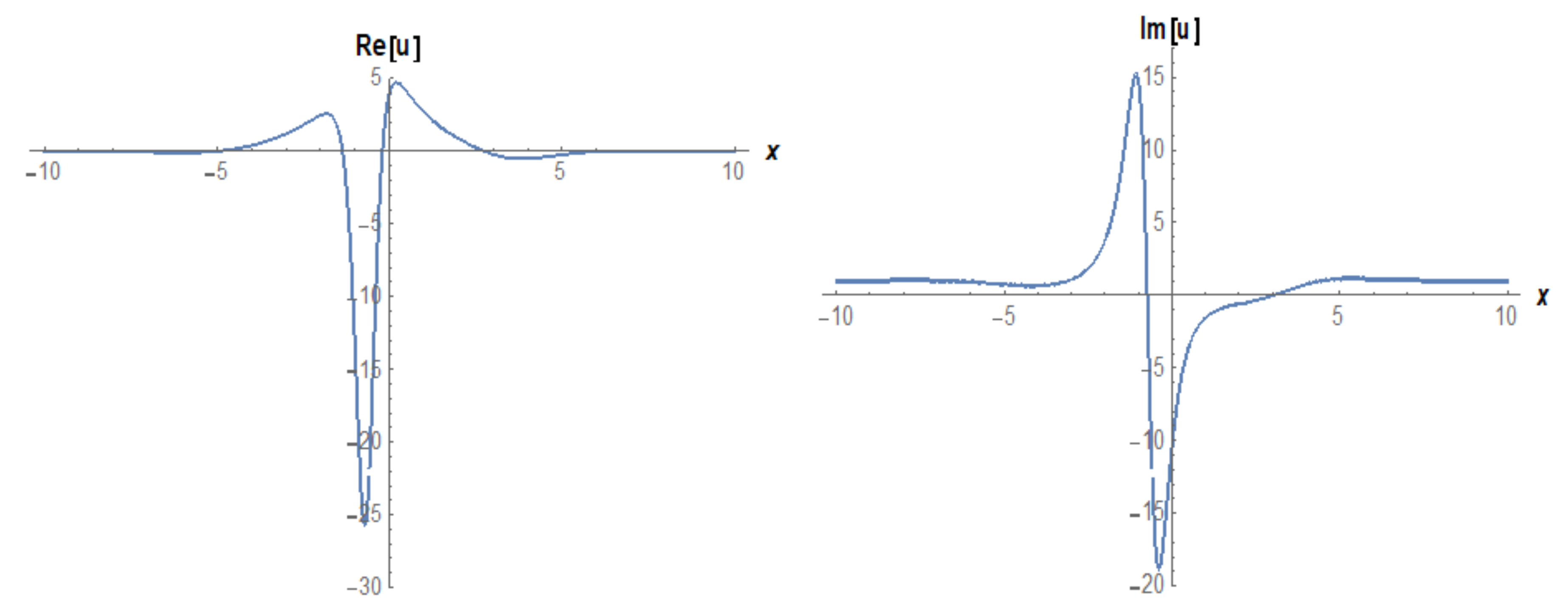
Figure 8.
The 3D surfaces of Equation (22) under the values of

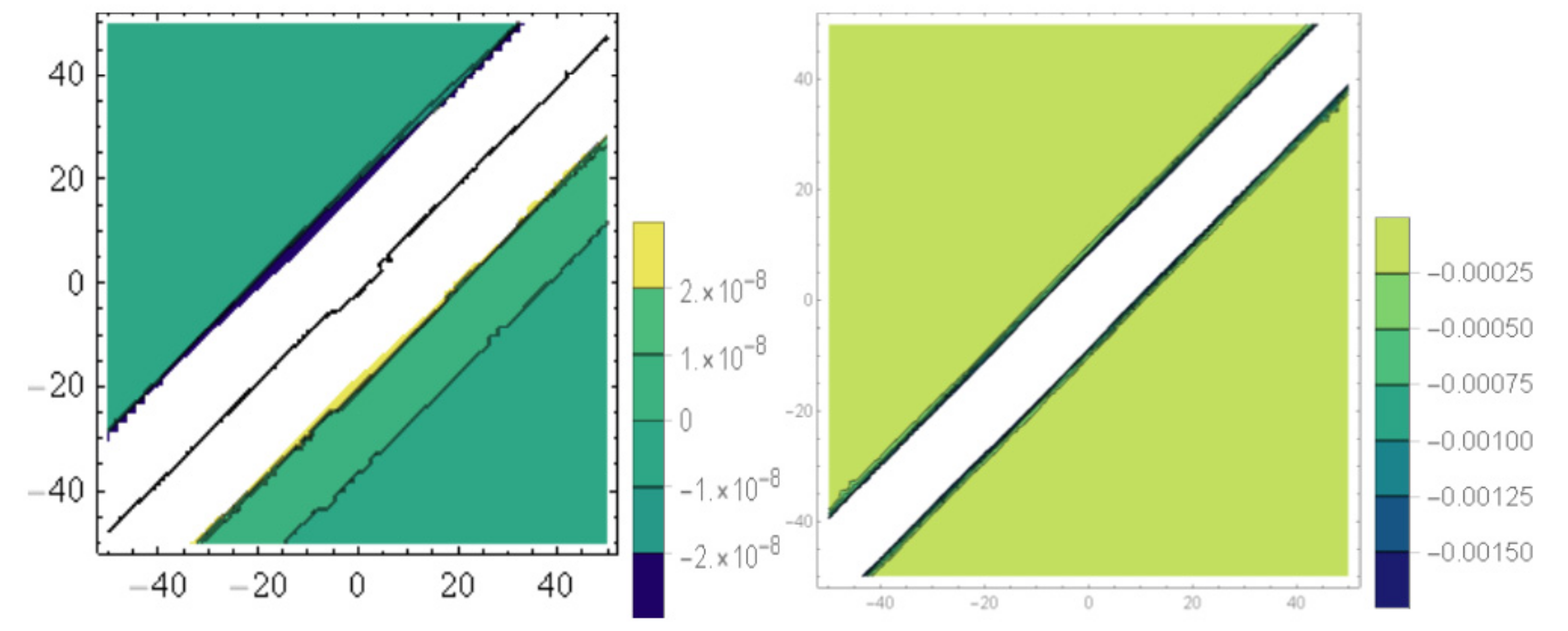
Figure 9.
The contour surfaces of Equation (22) under the values of

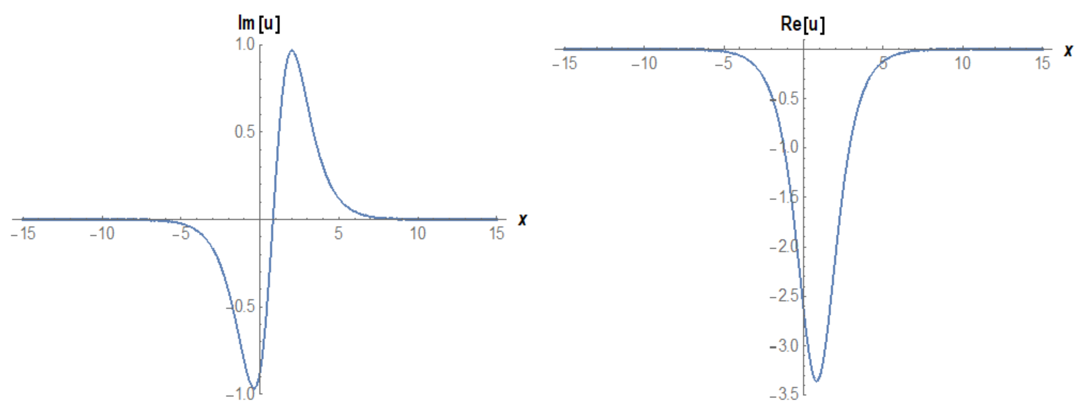
Figure 10.
The 2D surfaces of Equation (22) under the values of

Figure 11.
The 3D simulations of Equation (24) under the values of

Figure 12.
The contour graphs of Equation (24) under the values of

Figure 13.
The 2D graphs of Equation (24) under the values of

Figure 14.
The 3D simulations of Equation (26) under the values of

Figure 15.
The contour graphs of Equation (26) under the values of

Figure 16.
The 2D graphs of Equation (26) under the values of

Figure 17.
The 3D surfaces of Equation (30) under the values of .

Figure 18.
The contour surfaces of Equation (30) under the values of

Figure 19.
The 2D surfaces of Equation (30) under the values of

Figure 20.
The 3D surfaces of Equation (32) for

Figure 21.
The contour surfaces of Equation (32) for

Figure 22.
The 2D surfaces of Equation (32) for

Publisher’s Note: MDPI stays neutral with regard to jurisdictional claims in published maps and institutional affiliations. |
© 2021 by the authors. Licensee MDPI, Basel, Switzerland. This article is an open access article distributed under the terms and conditions of the Creative Commons Attribution (CC BY) license (http://creativecommons.org/licenses/by/4.0/).
Share and Cite
MDPI and ACS Style
Baskonus, H.M.; Ercan, M. Extraction Complex Properties of the Nonlinear Modified Alpha Equation. Fractal Fract. 2021, 5, 6. https://0-doi-org.brum.beds.ac.uk/10.3390/fractalfract5010006
AMA Style
Baskonus HM, Ercan M. Extraction Complex Properties of the Nonlinear Modified Alpha Equation. Fractal and Fractional. 2021; 5(1):6. https://0-doi-org.brum.beds.ac.uk/10.3390/fractalfract5010006
Chicago/Turabian StyleBaskonus, Haci Mehmet, and Muzaffer Ercan. 2021. "Extraction Complex Properties of the Nonlinear Modified Alpha Equation" Fractal and Fractional 5, no. 1: 6. https://0-doi-org.brum.beds.ac.uk/10.3390/fractalfract5010006