1. Introduction
Game theory is the study of mathematical models for describing competition and cooperation interaction among intelligent rational decision-makers [
1]. In the past few years, networked games have received increasing attention due to their wide applications in different areas such as competitive economy [
2], power allocation in interference channel models [
3,
4], environmental pollution control [
5], cloud computing [
6], wireless communication [
7,
8,
9], and adversarial classification [
10,
11].
The Nash equilibrium (NE) is a set of strategies where each player’s choice is its best response to the choices of the other players of the game [
12]. An NE in games with shared coupling constraints is referred to as generalized Nash equilibrium (GNE) [
13]. In order to compute the GNE, a great number of algorithms have been proposed [
14,
15,
16,
17,
18], most of which depend on
full-decision information, i.e., each player is assumed to have full access to all of the other players’ actions. However, such an assumption could be impractical in large-scale distributed networks [
19,
20]. To overcome this shortcoming, fully distributed algorithms under the
partial-decision information setting have recently become a research topic that attracts recurring interest.
Under the partial-decision information setting, each player can communicate only with its neighbors (instead of all its opponents) via a certain communication graph. In this case, the player has no direct access to some necessary decision information involving its cost function. In order to make up for the missing information, the player estimates other players’ actions and exchanges its estimates with neighbors. Such an estimate would tend to be the real actions of players by designing an appropriate consensus protocol [
21]. So far, some efforts have been devoted to the GNE seeking problem with partial-decision information. For example, an adaption of a fictitious play algorithm for large-scale games is introduced in [
22], and information exchange techniques for aggregative games are studied in [
23]. An operator-theoretic approach has been introduced to analyze GNE problems [
16,
21], under which the problem is cast as finding a zero of a sum of monotone operators through primal-dual analysis and show its convergence by reformulating it as a forward–backward fixed-point iteration.
Compared with the existing distributed algorithms for diminishing steps [
24], the algorithm for fixed steps has the potential to exhibit a faster convergence [
16]. Very recently, some distributed proximal algorithms and project-gradient algorithms have been proposed for seeking the GNE with fixed steps [
16,
25,
26,
27,
28]. It is worth noting that most of the existing algorithms, under the partial-decision information setting, require that the extended pseudo-gradient mapping in the augmented space of actions and estimates is strictly/strongly monotone. Such an assumption seems strong and how to relax it becomes a technical difficulty. In this paper, we would like to investigate the GNE seeking algorithm under a mild assumption of the extended pseudo-gradient mapping, like [
21].
In addition, some refined GNE seeking algorithms with inertia and relaxation have been proposed in ([
16], [Alg. 6.1]), ([
29], [Alg. 2]) and ([
25], [Alg. 3]) to accelerate the convergence to GNE. Although the fast convergence of the mentioned algorithms has been validated numerically, more computation resources are inevitably required at each iteration. Note that the computation resources could be limited and expensive in many situations. Inspired by the above discussion, in this paper, we combine a projection based algorithm via a doubly augmented operator splitting from the work [
21] with the inertia/overrelaxation idea from the paper [
25]. Specifically, we design distributed GNE seeking algorithms to balance the convergence rate and computation consumption in games with shared coupling constraints under a partial-decision information setting. Two kinds of fully distributed algorithms, i.e., alternating inertial algorithms and alternating overrelaxed algorithms, are proposed with fixed step-sizes. Their convergence to the GNE are guaranteed under a mild assumption on the extended pseudo-gradient mappings, compared to [
26], by using the Karush–Kuhn–Tucker (KKT) conditions of an optimization problem and variational inequality. Finally, a numerical example is provided to show the effectiveness of our algorithms that are validated numerically to have a relatively fast convergence rate.
The remainder of the paper is organized as follows. In
Section 2, we introduce some notations and backgroud theory.
Section 3 describes the problem that we are interested in, formulates it into mathematical model, and rewrites the game into a problem of finding the solution of the stochastic variational inequality (SVI). In
Section 4, we propose two alternating fully distributed GNE seeking algorithms under a partial-decision information setting and assumptions to guarantee convergence; the convergence analysis is also presented in this section. We present numerical results in
Section 5 and finally conclude in
Section 6.
Notations: Let represent an m-dimensional (non-negative) Euclidean space. is an dimensional vector with all elements equal to and is the identity matrix with dimension. denotes the N-dimension column vector with all elements equal to 1. We denote or as the Cartesian product of the sets . For given n column vectors , . Let denote the k-th element in column vector x, let denote the inner product of , and denotes the norm induced by the inner product . stands for a symmetric positive definite matrix. Similarly, the -induced product is , and the -induced norm is ⊗ is the Kronecker product, and denotes the block diagonal matrix with on its diagonal. Suppose , then where denotes the element of in the j-th row and k-th column.
3. Game Formulation
In this section, we build a mathematical setup about the problem considered.
Consider a set of players , where every player controls its local decision variable and is the private decision set of player i. Denote and , then the stacked vector of all the players’ decisions is called the decision profile. We also write , where denotes all of the decisions except player i’s.
The local objective function of each player
is denoted by
, and the affine coupling constrained set is defined as
where
and
Here,
and
are the local data only accessible to player
Define the feasible set of player
i as
, which implies that the feasible set of each player depends on the action of the other players. Every player aims to optimize its objective function, and the game can be represented by the inter-dependent optimization problems
Definition 1. A GNE of game (3) is a collective strategy such that for all In order to deal with the coupling constraints and solve the problems, we define the Lagrange function of each player
:
where
is a dual variable. According to optimization theory, if
is an optimal solution to (
3), then there exists
such that the following KKT conditions are satisfied:
By using the normal cone operator, the KKT conditions (
6) are equivalent to
Note that by the definition of a normal cone, one has
when
, which implies
(equivalently
) when (
7) holds. Furthermore,
, that is, if
, then
, and thus
; if
, then
, and hence
. This result implies that
and
.
We consider the GNE with the same Lagrangian multipliers for every player, i.e.,
, which is called
variational GNE (v-GNE). The v-GNE
is a solution of the following inequality
where
F is the
pseudo-gradient mapping of the game with the following form:
Assumption 1. Given , is continuously differentiable and convex in , and is nonempty, compact and convex for each player i, then K is nonempty and satisfies Slater’s constraint qualification.
Assumption 2. F is μ-monotone and -Lipschitz continuous, i.e., for any point x and , and .
It follows from ([
15], [Theorem 4.8]) that
solves
(
8) if and only if there exists a
such that the KKT conditions are satisfied:
where
.
Assumption 1 guarantees the existence of the v-GNE for game (
3) by ([
31], [Corollary 2.2.5]). The goal of this paper is to design distributed algorithms for seeking the v-GNE under a
partial-decision information setting, where both the computational cost and convergence rate are taken into consideration.
4. Alternating Distributed v-GNE Algorithms
In this section, we propose two kinds of distributed algorithms for seeking the v-GNE of game (
3) with partial-decision information, where each player controls its own actions and exchanges information with its neighbors via the communication graph.
Remark 1. Some GNE seeking algorithms with inertia and overrelaxation have been proposed [
28,
29].
Although the fast convergence of these algorithms has been validated numerically, more computation resources are inevitably required at each iteration. Note that the computation resources could be limited and expensive in many situations. Inspired by the above discussion, in this section we design distributed GNE seeking algorithms with alternated inertia and alternated overrelaxation, where both fast convergence rate and low computation consumption are taken into consideration. Suppose that player
controls its local decision
and
(i.e., the estimation of
in (
10)). In order to make up for the lack of non-neighbors’ information, we introduce an auxiliary variable
for each player
i that provides the estimation of the other players’ decisions. To be specific,
where
denotes the player
i’s estimation of player
j’s decision and
. We can also rewrite
, where
represents player
i’s estimation vector except its own decisions. In addition, an auxiliary variable
is introduced for each player
We assume that each player exchanges its local variable
with its neighbor through the communication graph
Assumption 3. The communication graph is undirected and connected.
4.1. Alternating Inertial Distributed v-GNE Seeking Algorithm
In this subsection, we propose an alternating inertial distributed algorithm for seeking the v-GNE, where the inertia is adopted intermittently (see Algorithm 1). Here, and denote at iteration respectively, and denote at iteration respectively. is the inertial parameter, c is the coupling parameter, and are the fixed step-sizes of player i in the update step. is the projection operator on to the set .
Let and Let with and In addition, , and
The
extended pseudo-gradient mapping
is defined as
Let
, where
, and we define operators
and matrix
as follows:
where
with
and
| Algorithm 1 Distributed alternating inertial v-GNE seeking. |
Initialization: Acceleration: Set if k is even, if k is odd.
|
Let
where
denote
,
,
,
,
,
at iteration
respectively. Suppose that
and
is maximally monotone, then Algorithm 1 is equivalent to
where
in (
12)–(
13),
and
Lemma 1. Suppose and is maximally monotone, then any limit point of Algorithm 1 is a zero of and a fixed point of .
Proof. By the continuity of the right hand of (
15),
. Since
is positive definite,
□
In order to show the convergence of the algorithm, the following assumptions are introduced.
Assumption 4. The extended pseudo-gradient mapping in (11) is θ-Lipschitz continuous, i.e., there exists such that for any and , . Let
with
,
in Assumption 2, and
in Assumption 4. Let
. It follows from ([
21], [Lemma 4]) that if
c is selected such that
, then
is maximally monotone and
is
-
restricted cocoercive, i.e., for any
and any
, where
,
where
, and
is the maximal weighted degree of
, i.e.,
.
Similar to [
21], a mild assumption (Assumption 4) on the pseudo-gradient mapping
is required only, while the requirement of strong monotonicity is relaxed for
.
Theorem 1. Suppose Assumptions – hold. Choose , and the step sizes , and . Then for any , the sequence generated by Algorithm 1 converges to the equilibrium , where and is a v-GNE of the game (3). Proof. It follows from the Gershgorin’s circle theorem ([
32], [§6.8 Theorem 1]) that, given any
is positive definite and
is positive semi-definite if the step sizes
and
Next, we first show the convergence of and then show the convergence of .
By ([
21], [Lemma 6]), we have
and
is
-
restricted averaged, i.e., for any
and any
,
It follows from ([
30], [Proposition 4.32]) that
is
-
restricted averaged, with
when
Let
be a fixed point of
T, then
according to ([
21], [Theorem 1]).
(i) For the subsequence
by (
15), we have
Then, by
T is
averaged, we obtain
By resorting to
and by using (
17) again, (
18) can be rewritten as
Choose
, then
This result implies that the sequence
is decreasing and non-negative, and thus converges. Moreover, we have
and
Note that since
is bounded, then there exists a convergent subsequence
that converges to
Obviously,
Let , we have , which implies that is a fixed point of T and thus converges. Since converges to 0, converges to
(ii)
T is
restricted nonexpansive since it is
-
restricted averaged, and then one obtains
which implies that the odd subsequence
also converges to
, and thus
converges to
Note that
and
is maximally monotone.
is a fixed point of
and hence is a zero of
by Lemma 1. It follows from ([
21], [Theorem 1]) that given any
, then
and
solves
(
8), that is,
is a v-GNE of game (
3). □
4.2. Alternating Overrelaxed Distributed v-GNE Seeking Algorithm
In this subsection, an alternating overrelaxed distributed algorithm is constructed for seeking the v-GNE, presented in Algorithm 2, and also that
is an overrelaxed parameter. Here the partial-decision information setting is considered.
| Algorithm 2 Distributed alternating overrelaxed v-GNE seeking. |
Initialization: Acceleration: Set if k is even, if k is odd.
|
Similar to (
15), we suppose that
and
is maximally monotone, then Algorithm 2 is equivalent to
where
and
T is given in (
15).
Next, we prove the convergence of Algorithm 2 to a v-GNE.
Theorem 2. Suppose Assumptions – hold. Take any , , and the step sizes , and . Then, for any , the sequence generated by Algorithm 2 converges to the equilibrium , where and is a v-GNE of the game (3). Proof. Similar to Theorem 1, we first show the convergence of and then prove the convergence of . Note that is -restricted averaged with when Let be any fixed point of
First, we consider the subsequence
and according to (
23) and (
17), one has
where the first equality holds due to
By choosing
, we have
which implies that
is monotonically decreasing and bounded, and is thus convergent. Furthermore,
that is,
, and hence
Note that if is bounded, there exists a convergent subsequence for some limit .
Let
in (
26), we have
which implies
is a fixed point of
T, thus
converges. Since
,
converges to
.
(ii) If
T is
restricted nonexpansive since it is
-
restricted averaged, then one obtains
which implies that the sequence
converges to the same limit of
, and thus
converges to
. □
5. Numerical Simulation
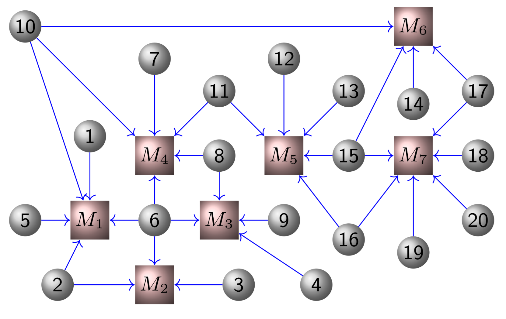
In this section, we consider a classic Nash–Cournot game over a network as [
21], where there are
N firms and each firm
produces commodities to participate in the competition over
m markets (see
Figure 1). Each market (denoted by
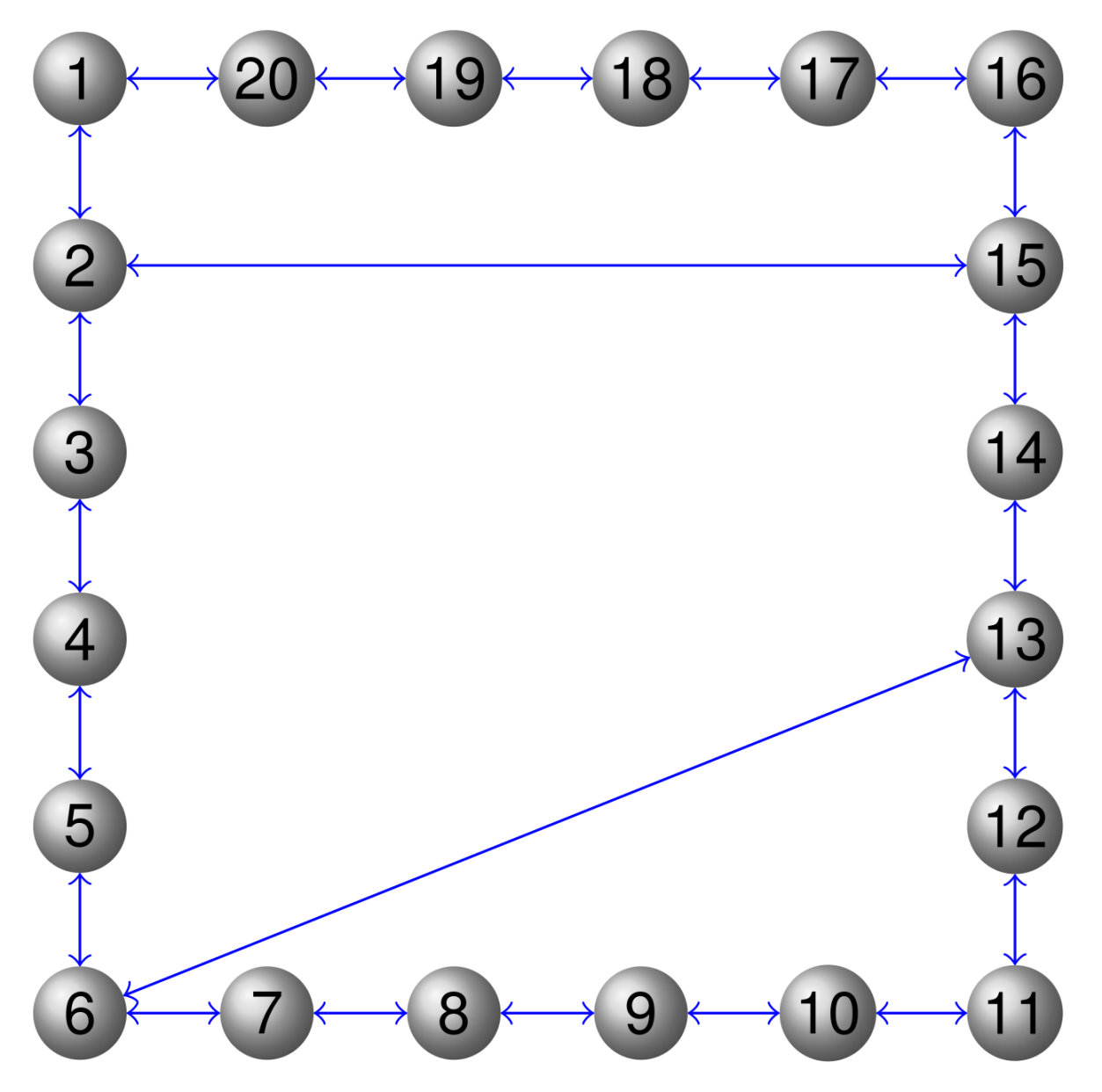
) has limited capacity. Here, the partial-decision information setting is considered where each firm has limited access to its neighboring firms’ information over the communication graph as in
Figure 2.
We assume that firm i participates in markets by producing amount of commodities and its production is limited by the set . The local matrix for firm i represents which markets it participates in. Specifically, for the j-th column of its k-th element is 1 if and only if firm i delivers amount of production to market all other elements are Each market has a maximal capacity of that is, , where and . Suppose that each firm i has the production cost and the price function maps the total supply of each market to the market’s price vector. The local objective function of firm i is .
Suppose and Let , where each component of is randomly drawn from . is randomly drawn from The local cost function of firm i is , where is a diagonal matrix with the elements randomly drawn from and is randomly drawn from . The price function is taken as the linear function with and where and are randomly drawn from and respectively. Set the step-sizes as and .
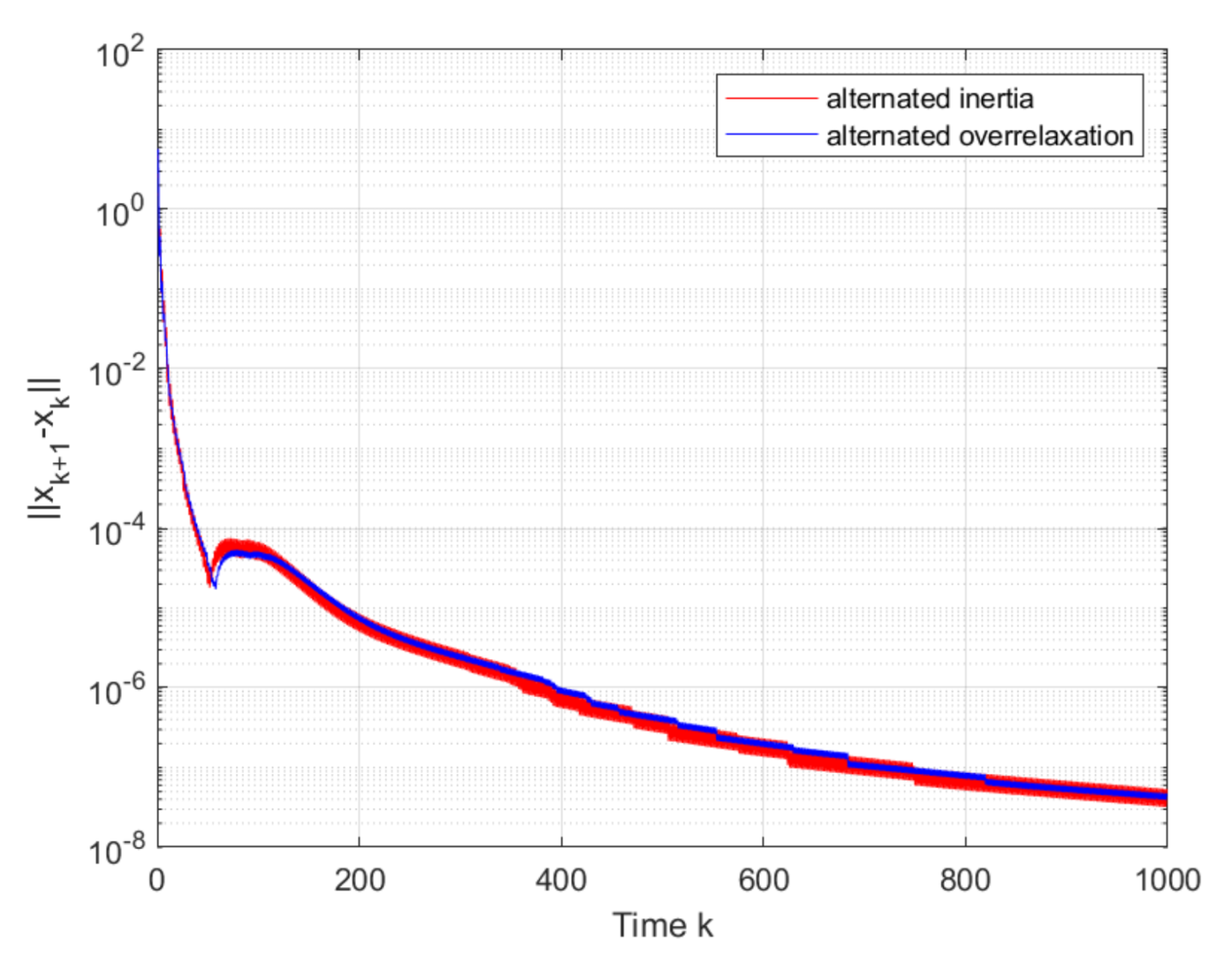
First,
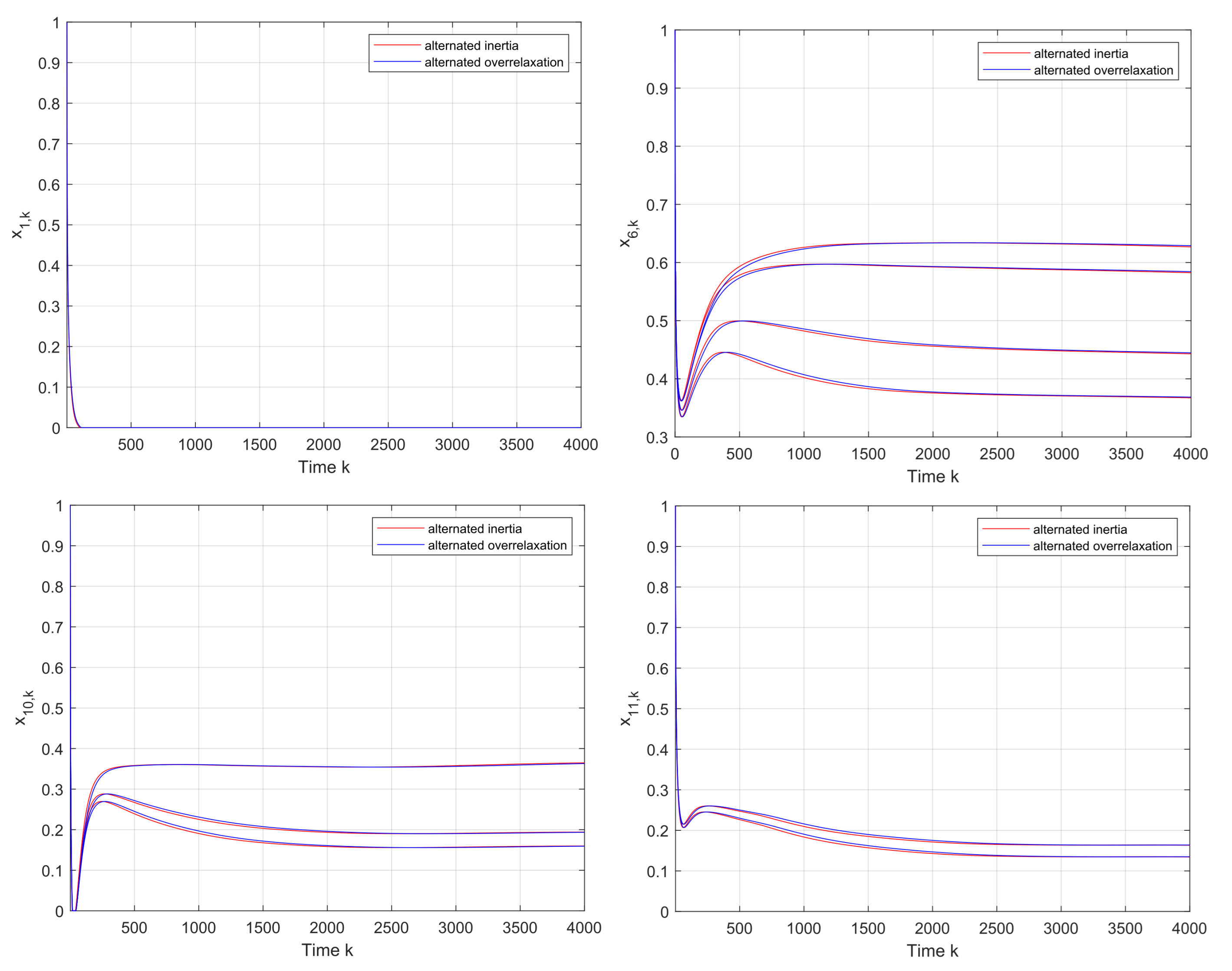
Figure 3 shows that the convergence to the v-GNE can be guaranteed under Algorithms 1 and 2, and the trajectories of the local decision
of firms
are displayed in
Figure 4. It can be seen in
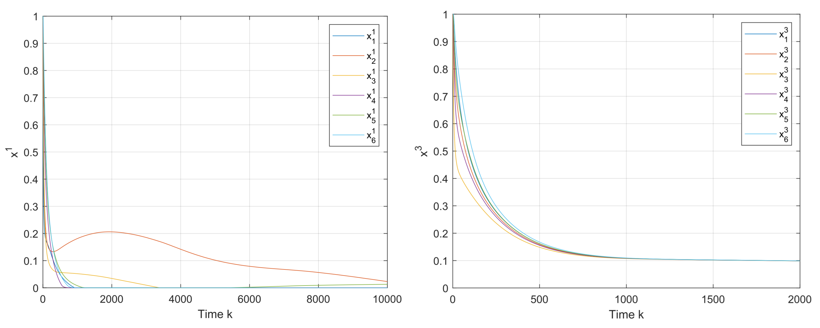
Figure 5 that the estimates on the firms 1 and 3 asymptotically tend to their real actions by using the proposed algorithms.
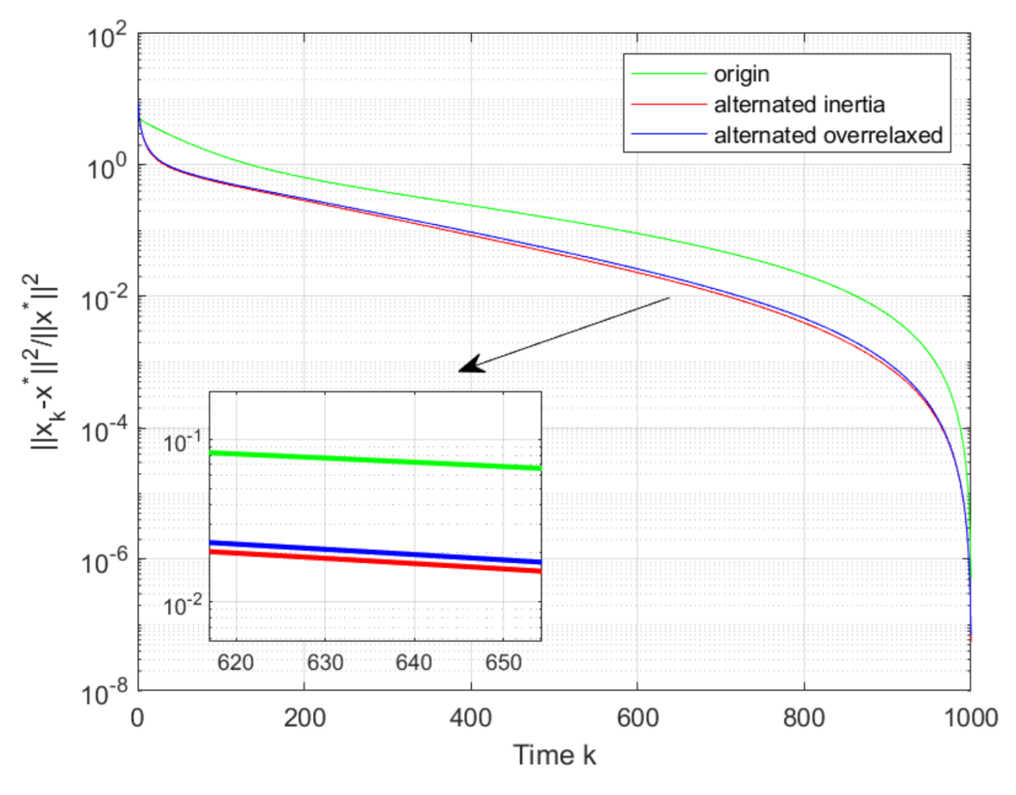
Then, it can be seen from
Figure 6, that both of the proposed Algorithms 1 and 2 converge to the GNE
with a faster convergence as compared with ([
21], [Alg. 1]), where Algorithm 1 has the fastest convergent rate. From
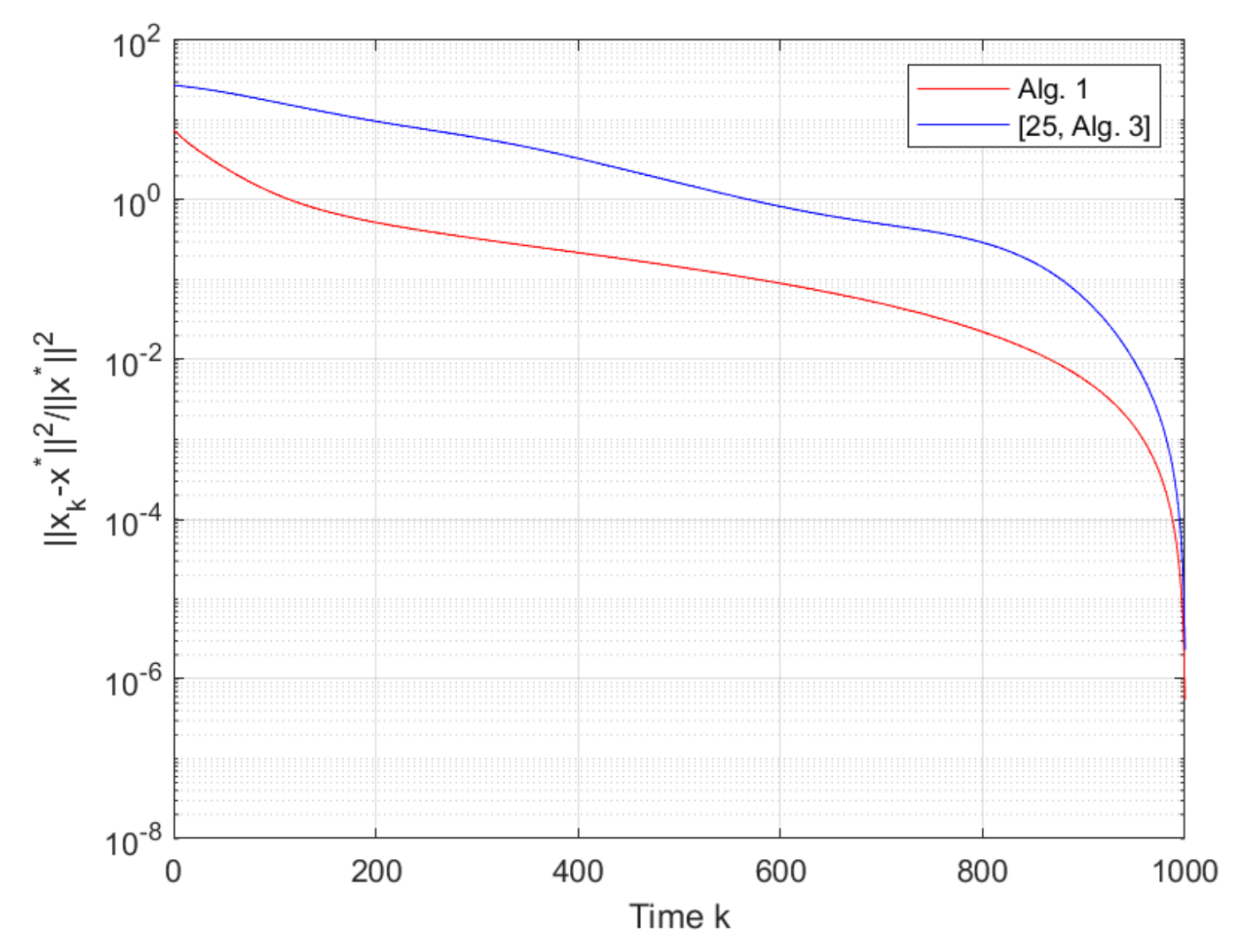
Figure 7 we can see that the proposed Algorithm 1 also has a faster convergence rate than ([
25], [Alg. 3]). We set
in ([
25], [Alg. 3]), the same step-sizes
and
and the same other parameters as Algorithms 1 and 2 in ([
21], [Alg. 1]) and ([
25], [Alg. 3]). On the other hand, as compared with the algorithm with inertia, Algorithm 1 with alternating inertia requires less computation resources. Thus, Algorithm 1 could be the best choice when both fast convergence rate and low computation cost are taken into consideration.
Remark 2. It is worthwhile to note that the introduction of the inertia and overrelaxation steps has the potential of accelerating the convergence rate. As such, in this paper, the inertial and overrelaxed distributed algorithms are developed based on the pseudo-gradient method for seeking generalized Nash equilibrium in multi-player games. The similar inertia idea has been considered in the proximal-point algorithm (see ([25], [Alg. 3])). However, the proximal-point algorithm generally needs to solve the optimization problem at each step k, which may be time-consuming and possibly costs a great amount of computation resources in many situations. As such, pseudo-gradient algorithms with inertia and overrelaxation were constructed in this paper, which successfully guarantees the convergence to v-GNE with a fast convergence rate. Moreover, we note that the introduction of the inertia and overrelaxation steps increases the computation burden, and thus two alternating inertial and overrelaxed algorithms are established in Algorithms 1 and 2 to balance the convergence rate and computation burden. In order to better display the effectiveness of our algorithms, we have added the comparison with ([25], [Alg. 3]) in the simulation part (see Figure 7). From Figure 7, it can be seen that Algorithm 1 in this paper outperforms the ([25], [Alg. 3]) in terms of the convergence rate. 


